Article

Free Electron Laser High Gain Equation and Harmonic Generation

ENEA—Frascati Research Center, Via Enrico Fermi 45, 00044 Rome, Italy
*
Author to whom correspondence should be addressed.
These authors contributed equally to this work.
Appl. Sci. 2021, 11(1), 85; https://doi.org/10.3390/app11010085
Submission received: 21 October 2020 / Revised: 16 December 2020 / Accepted: 17 December 2020 / Published: 24 December 2020

Abstract

:
The F E L integral equation is reviewed here and is studied under different contexts, accounting for diverse physical regimes. We include higher order harmonics and saturation effects, and explain the origin of scaling relations, widely exploited to describe either F E L dynamics or nonnlinear harmonic generation.

1. Introduction

This article describes an important mechanism associated with the physics of the free electron laser ( F E L ) regarding the nonlinear harmonic generation. The topic will be discussed by entering deeply into the mathematical aspects of what is currently referred as the high gain F E L equation.
A F E L is a laser device employing a beam of relativistic electrons injected into an undulator magnet, where it undergoes transverse oscillations and emits bremsstrahlung radiation, inversely proportional to the electrons energy square [1]. The F E L devices can be operated in the oscillator configuration by storing the emitted radiation in an optical cavity (whenever appropriate mirrors to confine the “light“ are available). The radiation moves back and forth inside the resonator and interacts, at each entrance inside the undulator, with a freshly injected e-beam, thereby becoming amplified. The intracavity intensity grows, round trip after round trip; it is amplified by the process of stimulated bremsstrahlung emission and exhibits the same pattern of conventional laser oscillators; it undergoes exponential growth, and eventually saturation occurs, when the gain is reduced by the nonlinear contributions to the level of the cavity losses.
In the region of the spectrum where efficient mirrors are not available, cavity-less operation is an obliged step. In this regime, the gain of the system should be sufficiently large to bring the device to saturation in one undulator passage. These F E L devices, nowadays devoted to the production of intense X-ray beams, require long undulators (hundreds of meters) and high energy (up to tens of GeV)/high brightness electron beams (namely, beams with high intensity peak current, low energy, angular and transverse spatial dispersions). The “single pass“ F E L devices may be operated in the amplifier configuration, when coherent input seeds are available; if not, the system works in the so-called self-amplified spontaneous emission ( S A S E ) regime. The electrons emit ordinary synchrotron radiation at the entrance of the undulator, which reinteracts with the electrons, becomes amplified and eventually reaches saturation.
The paradigmatic steps leading the F E L to the generation of coherent laser-like radiation are the beam energy modulation, the bunching, the exponential growth and the saturation.
These phases are common to all other free electron devices (such as gyrotrons and coherent auto-resonance masers), and most of the relevant theoretical and mathematical descriptions can be framed within the same context [2]. Many F E L s are presently operating and have operated in the past [3]. They are covering the electromagnetic spectrum from T H z region to X-rays. The last generation of F E L sources (sometimes referred as fourth generation synchrotron radiation sources) has opened up unprecedent scenarios in different research fields because of the radiation characteristics, in terms of brightness (ten orders of magnitude above the ordinary sources) and the shortness of the pulses [4,5,6,7].
The growth of the F E L field is ruled, in the small signal regime (namely, the dynamical conditions, when the field intensity is not large enough to induce nonlinear effects), by an equation known as the F E L integral equation; it is derived from the linearization of the pendulum equation, reported below [8,9,10,11,12,13,14,15,16].
d 2 d τ 2 ζ = a cos ( ζ + ϕ ) , d d τ a = j e i ζ , τ = z L , j = 2 π g 0 , a = a e i ϕ , ν = d d τ ζ
where z is the longitudinal coordinate; L is the undulator length; g 0 is the small signal gain coefficient; and a and j are Colson’s dimensionless amplitude and current respectively, ζ , ν the F E L longitudinal phase space variables and the brackets, denote the average of the phase space distribution. The use of dimensionless variables has several advantages. They constitute a set of comprehensive quantities such as a and g 0 , allowing one to merge all the significant F E L parameters into a single variable, providing quantities of interest (such as the gain and saturation intensity; see below) crucial in the descriptions and designs of F E L devices. The relevant small signal limit is achieved through the following approximations [17,18].
(a)
From the first of Equation (1), we obtain the lowest order (in the field strength) expansion of ζ , namely
ζ ζ 0 + ν 0 τ + δ ζ , δ ζ = 0 τ ( τ τ ) R e a ( τ ) e i ( ζ 0 + ν 0 τ ) d τ
where ν 0 = 2 π N ω 0 ω ω 0 is the detuning parameter.
(b)
Inserting δ ζ in the second of Equation (1) and averaging on the electron-field phase ζ 0 , we get
d d τ a = 2 π g 0 b 1 e i ν 0 τ + i π g 0 0 τ ( τ τ ) a ( τ ) e i ν 0 ( τ τ ) d τ + + i π g 0 b 2 0 τ ( τ τ ) a * ( τ ) e i ν 0 ( τ + τ ) d τ
where the averages have been taken by considering the e-beam mono-energetic and without spatial and angular dispersion, thereby getting
κ ( ζ 0 ) ζ 0 = 1 2 π 0 2 π f ( ζ 0 ) κ ( ζ 0 ) d ζ 0 , f ( ζ 0 ) = n = b n e i n ζ 0 , b n = e i n ζ 0 ζ 0 .
The physical meaning of Equation (3) is transparent; the three terms on the right-hand side account for three different regimes:
(i)
Absence of an initial bunching ( f ( ζ 0 ) constant); in this case Equation (3) reduces to
d d τ a = i π g 0 0 τ ( τ τ ) a ( τ ) e i ν 0 ( τ τ ) d τ .
The underlying physics is that energy modulation and consequent bunching are due to the input coherent seed a 0 .
(ii)
Nonconstant f ( ζ 0 ) and emergence of non zero b n coefficients; the field may grow in a seedless mode, induced by the initial bunching coefficient, as illustrated below.
In order to understand the role of the bunching coefficients during the early stages of the F E L interaction, we must treat Equation (5) in terms of a naïve expansion in the small signal gain coefficient, limiting ourselves to the second-order expansion in the small and neglecting b 2 ; then we find
a ( τ ) a 0 + g 0 a 1 + g 0 2 a 2 , a 0 ( τ ) = 0 , d d τ a 1 = 2 π b 1 e i ν 0 τ , d d τ a 2 = i π 0 τ ( τ τ ) a 1 ( τ ) e i ν 0 ( τ τ ) d τ
and the relevant solution is
a ( τ ) 2 π b 1 g 0 sin ν 0 τ 2 ν 0 2 e i ν 0 τ 2 1 2 π g 0 ( i ν 0 2 τ 2 + 4 ν 0 τ 6 i ) e i ν 0 τ + 6 i + 2 ν 0 τ ν 0 4 .
According to the previous equation, the field grows initially because of being triggered by the bunching coefficient. It provides a kind of coherent spontaneous emission, which in the second phase is responsible for the onset of the exponential growth regime (see Figure 1), where we have reported the combined effects of bunching and initial seed.
The previous results have been obtained using a perturbative expansion, which is not strictly necessary, since the F E L integral equation can be reduced to the ordinary differential equation reported below.
D ^ τ 3 + 2 i ν 0 D ^ τ 2 ν 0 2 D ^ τ a ( τ ) = i π g 0 a ( τ ) + b 2 a * ( τ ) e 2 i ν 0 τ , D ^ τ = d d τ ,
obtained after noting that integrals of type
i π g 0 0 τ ( τ τ ) a ( τ ) e i ν 0 ( τ τ ) d τ = i π g 0 e i ν 0 τ 0 τ 0 τ a ( τ ) e i ν 0 τ d τ d τ
appearing in Equation (6) are double integrals which can be eliminated by keeping two successive derivatives [17,18]. It is evident that, for negligible b 2 (we have checked that the second-order bunching coefficient does not produce any appreciable contribution and can be safely neglected), Equation (8) reduces to a naïve third-order ordinary differential equation, leading to the exponential growth also referred as F E L instability, the characteristic of which occurs in any Free Electron device [19,20,21,22,23,24,25]. (This type of instability is common to any free electron device (including gyrotrons and cyclotron auto-resonance masers ( C A R M )). This was widely established before the studies developed in the previously quoted references. Some interesting papers within this respect are listed in the bibliography.)
It is worth noting that, even though not explicitly contributing to Equation (8), the bunching coefficient b 1 appears in the initial conditions provided by
a ( 0 ) = a 0 , D ^ τ a τ = 0 = 2 π g 0 b 1 , D ^ τ 2 a τ = 0 = 2 π i ν 0 g 0 b 1 .
We have so far fixed the mathematical formalism to treat the problems associated with the effect of the bunching on the high gain (and not only) F E L evolution. The paper outline is reported below.
In Section 2 we discuss solution methods to deal with either the integral and third-order differential equation.
In Section 3 we deal with the extension of the integral equation to the harmonic generation and include effects associated with nonlinear regime.
Section 4 is finally devoted to application of the formalism for the design of F E L , exploiting segmented undulator devices.

2. Algorithmic and Analytical Solutions of the FEL Integral Equation

The equations we have dealt with in the previous section describe the 1 D small signal F E L dynamics, with the assumption of an ideal, sufficiently long beam such that short pulse effects can be neglected. The last assumption allows one to ignore the possible detrimental effects to the slippage, which will be considered later in this paper.
Within the present context, they are sufficiently general to develop useful considerations on the role of a pre-bunched e-beam on the F E L dynamics. We have also noted that Equation (3) can be reduced to a straightforward cubic equation, that analytical solutions are possible and that interesting information is obtained by the use of a perturbative expansion. The analysis has been so far limited (see Equation (7)) to a second-order expansion in terms of the small signal gain coefficient. The perturbative solution of Equation (5) can be obtained by including the higher order terms in g 0 , which yields the following recursion:
d d τ a n = i π 0 τ ( τ τ ) a n 1 ( τ ) e i ν 0 ( τ τ ) d τ , a n ( 0 ) = δ n , 0 .
We will go back to perturbative treatments in the forthcoming sections of this article; here we consider the use of the other means based allowing either algorithmic and analytical solutions.
Regarding the first, we consider a method outlined in a paper by F. Ciocci et al. [26]; the procedure will be referred to as the Ciocci algorithm ( C A ). The technique is used via the following steps:
(i)
The solution of the cubic equation can be written as
a ( τ ) = e i ν 0 τ j = 1 3 κ j e i δ ν j τ
where δ ν j are the roots of the third-degree algebraic equation
δ ν 2 ( ν 0 + δ ν ) = π g 0 ;
(ii)
The amplitudes κ j are fixed by the initial conditions, as shown below.
a ( 0 ) = α 0 = j = 1 3 κ j , d d τ a τ = 0 = i ν 0 α 0 i j = 1 3 κ j δ ν j = 2 π g 0 b 1 j = 1 3 κ j δ ν j = α 1 = ν 0 α 0 2 i π g 0 b 1 , d 2 d τ 2 a τ = 0 = ν 0 2 α 0 2 i ν 0 j = 1 3 κ j δ ν j j = 1 3 κ j δ ν j 2 j = 1 3 κ j δ ν j 2 = α 2 = ν 0 2 α 0 + 2 i π ν 0 g 0 b 1 .
(iii)
Equation (12) is cast in the more convenient form
a ( τ ) = e i ν 0 τ m = 0 ( i ) m m ! α m τ m , α m = j = 1 3 κ j δ ν j m .
(iv)
The coefficient α m is obtained from Equation (13). It can be written as
ν 0 δ v j 2 + δ ν j 3 = π g 0
which after multiplying by κ j and summing on the index j, yields the recursion
α 3 = π g 0 α 0 ν 0 α 2 ,
and which for the higher order terms ( m > 2 ) is generalized as
α m = π g 0 α m 3 ν 0 α m 1 ,
The solution of the cubic equation via C A is easily implemented numerically; it is extremely fast and yields the results contained in Figure 2 reporting the cases of seeded operation and bunching.
The intensity evolution vs. z for a seedless evolution ( α ( 0 ) = 0 , b 1 0 ) and for the amplifier configuration is reported in Figure 2a,b. The ν 0 , τ surfaces yield an idea of the small signal intensity evolution, and further comments will be provided below.
Analytic solutions can be obtained too; they require some algebra, and in particular the use of Cardano’s method to get the solution of Equation (13). Putting everything together we find:
(a)
The Fang–Torre formula (this Formula appeared in an unpublished manuscript by H. Fang, and was later derived with minor refinements by A. Torre, and reported in [27]) valid for a 0 0 , b 1 = 0 :
a ( τ , ν 0 ) = a 0 3 ( ν 0 + p + q ) e 2 i 3 ν 0 τ ( ν 0 + p + q ) e i 3 ( p + q ) τ + 2 ( 2 ν 0 + p + q ) e i 6 ( p + q ) τ · · cosh 3 6 ( p q ) τ + i 3 ν 0 p q sinh 3 6 ( p q ) τ , p = 1 2 ( r + d ) 1 3 , q = 1 2 ( r d ) 1 3 , r = 27 π g 0 2 ν 0 3 , d = 27 π g 0 ( 27 π g 0 4 ν 0 3 ) .
The square modulus of a ( τ , ν 0 ) yields the intensity growth as a function of the dimensionless time and of the detuning parameter. Regarding Equation (19) we find
a ( τ , ν 0 ) 2 = a 0 2 9 ( ν 0 + s + ) 2 4 ( 2 ν 0 + s + ) 2 cosh 3 6 s τ 2 + 3 ν 0 2 s 2 sinh 3 6 s τ 2 + + ( ν 0 + s + ) 2 + 4 ( ν 0 + s + ) ( 2 ν 0 + s + ) cos s + 2 τ cosh 3 6 s τ + 3 ν 0 s sin s + 2 τ sinh 3 6 s τ , s ± = p ± q .
We have very loosely described in introductory remarks the S A S E regime or seedless operation. In this case the field grows from a kind of prebunching characterizng the beam itself [28,29].
(b)
The field growing from a bunching coefficient associated with the electron distribution and the solution of the evolution problem reads:
a ( τ , ν 0 ) = 2 π g 0 b 1 Δ e i 2 3 ν 0 τ μ e i 3 ( p + q ) τ + χ cosh 3 6 ( p q ) τ + χ + sinh 3 6 ( p q ) τ e i 6 ( p + q ) τ , Δ = 3 9 ( p 3 q 3 ) , μ = i 3 9 ν 0 ( p + q ) ( p q ) , χ = 1 6 ν 0 + 1 2 ( p + q ) i 3 2 ( p q ) p + q + i 3 3 ( p q ) , χ ± = χ ± χ * .
Before proceeding further, we write Equation (21) in a form more appropriate for high gain/ S A S E F E L operation. To that end, we remind the reader that the small signal gain coefficient and Pierce parameter ρ (see references [8,9,10,11,12,13,14,15,16]) are linked by the identity
ρ = π g 0 3 4 π N ,
where N is the number of undulator periods. The intensity field growth is ruled by the so-called gain length
L g = λ u 4 π 3 ρ ,
which is the pivotal quantity controlling the small signal high gain dynamics; its inverse defines the growth per unit length. With these remarks in mind, we note that:
(i)
Quantities such as ν 0 and τ should be replaced by
ν 0 ν 0 ˜ = ν 0 4 π N 3 ρ = 1 2 3 ρ ω 0 ω ω 0 , τ z ˜ = z L g
and it is worth noting that the number of undulator periods does not appear anymore in the definition of the new dimensionless quantities (see below for further comments);
(ii)
Quantities involving the product of p , q and τ , written in the new variables, read
p τ = 3 1 + 1 4 ν ˜ 0 3 1 2 ν ˜ 0 3 3 z ˜ , q τ = 3 1 1 4 ν ˜ 0 3 1 2 ν ˜ 0 3 3 z ˜ .
It is finally important to stress that the Colson’s dimensionless amplitude in terms of dimensional quantities reads
a = 2 2 π I I s
where I is the field intensity (power/surface) and I s is the saturation intensity [30,31,32,33], a quantity which, in the theory of lasers, is exploited as a reference quantity to fix the onset of saturation. Even though its use is more appropriate for F E L operating in the oscillatory configuration, it can be exploited within the context of cavity-less operation too. Its dependence on the F E L parameters is specified by (practical units)
I s M W c m 2 = 6.9312 · 10 2 γ N 4 λ u [ c m ] K f b ( ξ ) 2 , ξ = 1 4 K 2 1 + K 2 2 .
A more appropriate expression for the high gain/ S A S E regime can be obtained by expressing the second of Equation (1) in the new dimensionless coordinates, thereby finding
d d z ˜ a ˜ = 2 3 e i ζ , a ˜ = 2 2 π I I ˜ s , I ˜ s M W c m 2 = 6.9312 · 10 2 ( 4 π γ ρ ) 4 λ u [ c m ] K f b ( ξ ) 2 .
For actual values of the F E L parameters entering in the definition of I ˜ s , we obtain for it reference numbers not dissimilar from the F E L saturated power, as discussed later in this paper.
The use of the previous variables allows one to cast the intensity evolution in the dimensional form (valid for ν 0 = 0 ) [17,18]
A ( z ˜ ) = 1 9 3 + 2 cosh z L g + 4 cos 3 2 z L g cosh z 2 L g , I ( z ˜ ) = I 0 A ( z ˜ ) , I 0 = I ˜ s 8 π 2 a 0 2 .
which has been largely exploited in the past [17,18] to describe the small signal F E L evolution; early derivations of similar equations trace back to the early eighties of the 20th century [34].
In Figure 3 we have plotted Equation (29) and the mere exponential behavior, which allows the conclusion that the region before the onset of the exponential growth, usually called lethargic region, lasts about two gain lengths, namely,
Z L 2.1 L g .
In any F E L device the small signal gain is a crucial parameter; it is naively defined as the relative intensity variation:
G = a ˜ ( z ˜ , ν ˜ 0 ) 2 a ˜ 0 2 a ˜ 0 2 .
In the case of low gain, its maximum value is proportional to the small signal gain coefficient through the well known identity [17,18]
G * = 0.85 g 0 .
Such a quantity measures the amplification of the input seed at the end of the undulator. We can, however, extend the concept by considering the same gain measurement at different points inside the undulator, as shown in Figure 4, after a number of periods
N z = z λ u .
We can therefore write G * in terms of ρ , z as (see Equation (32))
G * = 0.85 π z ˜ 3 3 .
The low gain regime relies on the assumption that the laser amplitude remains constant during the transit inside the undulator. The approximation breaks when higher order terms in g 0 are to be taken into account to specify the maximum gain at a given point in z. These corrections, derived in [35], can be written as
G * = a ˜ ( z ˜ , ν ˜ 0 * ) 2 a ˜ 0 2 a ˜ 0 2 0.85 π z ˜ 3 3 + 0.19 π 2 z ˜ 3 6 + 4.23 · 10 3 π 3 z ˜ 3 9 + o ( ρ 12 )
whose meaning is better explained in Figure 4, where we have also reported the departure of the gain line shape from the anti-symmetric curve, characterizing the early F E L experiments [36,37].
In this section we have provided a fairly general analysis describing the solution of the F E L high gain small signal equation.
In the forthcoming section we discuss how the technique we have discussed so far can be extended to the treatment of F E L induced higher order harmonics.

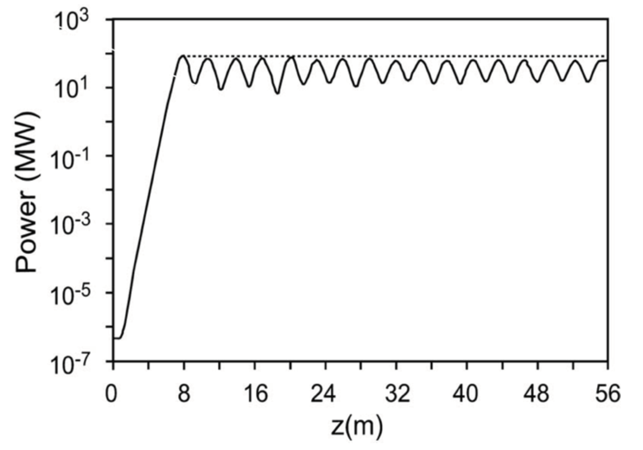
3. High Gain FEL Equations and Harmonic Generation

In this section we discuss the mechanism of harmonic generation in F E L devices, which is a process “naturally“ associated with the evolution of the fundemental harmonic. The importance of these further contributions in developing tools extending the capabilities of F E L s was soon recognized in the community, but the practical implementations took some time.
The pendulum equations, including the higher order harmonics, can be written as (differently from the index n in the perturbative terms discussed in Equation (11); in this case n is just the order of the harmonic) [38]
d 2 d τ 2 ζ = n = 0 a n cos ( ψ n ) , ψ n = n ζ + ϕ n , d d τ a n = j n e i n ζ , j n = 2 π g 0 , n
where a n = a n e i ϕ n is the dimensionless amplitude of the n-th order harmonics and g 0 , n is the n-th harmonic small signal gain parameter to be specified later [39].
d d τ a n = 2 π g 0 b n e i ν n τ + i π n g n 0 τ ( τ τ ) a n ( τ ) e i ν n ( τ τ ) d τ , ν n = 2 π N n ω 0 ω n ω 0 .
It is evident that the same considerations developed for the fundamental harmonic ( n = 1 ), hold in the present case too, the only significant difference being that the n-the harmonic Pierce is now specified by
ρ n * = n 3 ρ n , ρ n = ρ f b , n f b 2 3 , f b , n = J n 1 2 ( n ξ ) J n + 1 2 ( n ξ ) , f b , 1 = f b .
The gain length determining the harmonic linear growth is
L g , n * = λ u 4 π 3 ρ n * = 1 n 3 L g , n .
where L g , n is defined in terms of ρ n as
L g , n = λ u 4 π 3 ρ n
The role of L g , n * in the harmonic generation is clarified below; it is just a consequence of the assumption (summarized in Equation (36), where the electron field phase ψ n is written as n ζ ) that the process is dominated by the bunching induced by the fundamental harmonic.
It is worth noting that the correction term n 3 in the definition of the harmonic Pierce parameter was initially suggested in references [17,18,39] as a consequence of an accurate analysis of the numerical data from the code PROMETEO [40].
In Figure 5 we have reported the harmonic intensity growth vs. the longitudinal coordinate; the relevant behavior is the same as for n = 1 , reproduced by equations of the type (29) with L g , n * in place of L g .
However, this is only a part of the story. The harmonic intensities ( 3 ,   5 ) follow a growth rate characterized by two different regimes. After the lethargic region, the growth rates is initially specified by the inverse of the harmonic gain length L g , n * and then by an abrupt increase of the growth ruled by n L g 1 . This behavior is the signature of a complex mechanism underlying the harmonic generation emission.
We have so far considered the harmonic linear dynamics, in which within certain limits (to be discussed in the final section), the evolutions of the associated intensities are independent. It should be noted that harmonics too can be triggered by a bunching coefficient, as implicitly contained in Equation (37). As it is well known, the bunching grows with the intensity itself; the dynamics of each harmonic are the result of intrigued feedback between induced bunching and higher order-bunching (namely, at higher values of n). We crudely describe the process by noting that each harmonic, while the intensity grows, induces further bunching, determining the onset of the sub-harmonics m of the n-th harmonic—namely, the first harmonic indices higher order harmonics and each of them determines a further set of harmonics. In terms of bunching coefficients, we have: The fundamental harmonics ( n = 1 ) contributes to the increase of the bunching of order 1 and of other higher order bunching coefficients. The same holds for the higher order harmonics; the third is, e.g., responsible for the bunching of its own harmonics ( 3 , 6 , 9 , with respect to the fundamental).
The bunching process is not “free,“ and indeed an energy spread, associated with gain degradation and saturation mechanisms, is produced. This phenomenology is not considered within the present context.
The inclusion of nonlinear terms in our analysis occurs by keeping intensity dependent terms [17,18,41] which allow the following redefinition of the F E L integral equation:
d d τ a = 2 π g 0 e i ν 0 τ m = ( i ) m b 1 m J m Π Π m 0 τ ( τ τ ) a ( τ ) e i ν 0 τ d τ m , 0 τ ( τ τ ) a ( τ ) e i ν 0 τ d τ = Π e i ψ
where
J m Π = r = 0 ( 1 ) r r ! ( m + r ) ! Π 2 m + 2 r .
If we consider a perturbative solution of the above equation in terms of the fundamental intensity, we can write the first three terms as
d d τ a l = 2 π g 0 b 1 e i ν 0 τ + i π g 0 0 τ ( τ τ ) a l ( τ ) e i ν 0 ( τ τ ) d τ , d d τ a n l , 2 = 2 π g 0 e i ν 0 τ b 1 8 0 τ ( τ τ ) a l ( τ ) e i ν 0 τ d τ 2 , d d τ a n l , 3 = 2 π g 0 e i ν 0 τ b 2 2 3 3 ! 0 τ ( τ τ ) a 0 ( τ ) e i ν 0 τ d τ 3
which have been derived using the limit lim Π 0 J m Π Π m = 1 m ! 2 m . The subscripts l and n l stand for linear and nonnlinear, respectively. The n l -contributions stand for the onset of the nonnlinear harmonic generation.
Considering a linearly polarized undulator not providing coupling to even on axis harmonic generation, we obtain from the third Equation (43)
a n l , 3 = 2 π g 0 b 2 2 3 3 ! 0 τ e i ν 0 τ h 3 ( ν 0 , τ ) d τ , h 3 ( ν 0 , τ ) = 0 τ ( τ τ ) a 0 ( τ ) e i ν 0 τ d τ 3 .
Keeping the fast growing root only and assuming ν 0 = 0 , we find a further contribution to the harmonic intensity depending on the power of the fundamental and characterized (as already anticipated) by the gain length
L g ( n l h g ) = L g n
where n l h g stands for nonnlinear-harmonic generation.
The conclusion of this discussion is that there are two distinct contributions to the higher order harmonic emission. The first is a kind of lasing on harmonic; this concept was originally introduced in [42] by Colson et al., where the possibility of exploiting this mechanism to sustain higher order harmonics lasing in the oscillator configuration has been discussed. The second provides the well-known nonlinear harmonic generation mechanism; it goes beyond the linear analysis; its characterizing features and scaling relations are further discussed in the final section of this paper.
We have commented on the importance of the harmonic generation mechanism, which has opened the possibility of extending the relevant performances in terms of tunability range and not only.
We want to mention an important application of the harmonic generation in F E L which has determined a significant improvement of the relevant performances. It has already been underscored that running the F E L in the amplifier configuration is feasible if a coherent seed at certain wavelengths is available. This happens with F E L harmonics too, which can be triggered using the seeds from harmonic generation in gas (see references [43,44] for an adequate description). In these devices, the beam of laser (a Ti:sapphire laser, for example), is focused into a xenon gas cell, where high harmonic generation occurs. The output seed beam is then spatially and temporally overlapped to the electron beam moving in an undulator with the period chosen to match the seed frequency. The F E L harmonics then grow according to the mechanisms we have just outlined. The successful implementation of this concept has allowed the possibility of extending the F E L tunability of more than an order of magnitude (for more details, see [43] and references therein). A further idea, concerning the use of segmented undulators, after the beam self induced prebunching, is discussed in the forthcoming section.

4. Inhomogeneous Broadening Partial Amplitudes and High Gain FEL Equation

The high gain integral equation becomes slightly more complicated if the effect of non ideal e-beam qualities is included. The averages in Equation (2) need to be extended to the beam distribution (energy, spatial, angular, etc.). With these premises and limiting ourselves to the effect of the energy spread only, we find [45]
d d τ a = i π g 0 0 τ a ( τ τ ) τ e i ν 0 τ 1 2 ( π μ ε τ ) 2 d τ , μ ε = 4 N σ ε
obtained after taking the average of a Gaussian relative energy distribution with r.m.s. σ ε .
The solution of Equation (46) cannot be obtained in analytical terms; however, the method of partial amplitude expansion pioneered by A. Segreto in references [46,47] yields a fairly useful analytical mean allowing the solution of, e.g., Equation (46) in the form (we use the ν ˜ 0 , z ˜ variables, more appropriate for the forthcoming discussion)
a ˜ ( z ˜ , ν ˜ 0 ) = a ˜ 0 1 + k = 1 i k z ˜ 3 3 k g k ( z ˜ , ν ˜ 0 , μ ˜ ε ) , g k ( z ˜ , ν ˜ 0 , μ ˜ ε ) = M k γ k Σ k exp ( μ ˜ ε z ˜ ) 2 ( β k + i ξ k ( ν ˜ 0 z ˜ ) ) + 12 ( i λ k ( ν ˜ 0 z ˜ ) + ( ν ˜ 0 z ˜ ) 2 ) 24 Σ k 2 , M k = 1 ( 3 k ) ! , γ k = ( 3 k + 1 ) 3 k + 2 2 k ( k + 1 ) , Σ k = γ k 2 + 1 12 ( μ ˜ ε z ˜ ) 2 , β k = 2 4 k + 1 k + 1 , λ k = 2 ( 3 k + 1 ) 3 k + 2 k + 1 , ξ k = 2 ( 2 k + 1 ) ( k 1 ) ( k + 1 ) ( 3 k + 1 ) .
The previous equation can be profitably used to get information of a practical nature. The low gain expansion ( k = 1 ) yields for the intensity growth
a ˜ ( z ˜ , ν ˜ 0 ) 2 a 0 ˜ 2 1 + 2 M 1 3 3 Σ 1 z ˜ 3 · exp β 1 μ ˜ ε 2 + ν ˜ 0 2 24 Σ 1 2 z ˜ 2 sin ν ˜ 0 12 λ 1 + ξ 1 ( μ ˜ ε z ˜ ) 2 24 Σ 1 2 z ˜
which provides an idea of the interplay between inhomogeneous broadening and the other mechanisms contributing to the laser evolution. In Figure 6 we have reported the analogues of Figure 2b for different values of the inhomogeneous broadening parameter. The plot yields quite a good description of how the intensity growth is diluted by the presence of a non zero energy spread.
Other effects due to angular and spatial distribution of the electron beam can be introduced too. From the conceptual point of view, they do not imply any problem, but for the introduction of a further convolution term in Equation (46). The induced detrimental effects are expressed through appropriate μ -parameters, analogous to those associated with the energy spread. They are listed in [18].
It is important to stress that, from the practical point of view, the effect of non perfect electron beam qualities produces an increase of the gain length, which can be parameterized as [17,18]
L g ( μ ˜ ε ) = 1 + 0.185 3 2 μ ˜ ε 2 L g
The interest in the method of partial amplitudes stems also for the fact that it can be generalized to more complicated situations, involving, e.g., the pulse propagation contributions.
In the following we make the assumption that the electron bunch is sampled into a series of slices with a longitudinal size of the order of a coherence length [48,49,50]:
λ c = λ 4 π 3 ρ .
During the interaction the radiation is mismatched with respect to the electron bunch reference by a quantity depending on the slippage length. The computation of this aspect of the problem requires a certain amount of computation which, for the homogeneous case (no energy spread) has been accomplished in [51] and for the present case is summarized below.
According to the aforementioned reference and to the analytical steps outlined in [46,47], the problem is solved, in relatively easy terms, by replacing the detuning parameter with the operator
ν ˜ 0 ν ˜ ^ 0 = ν ˜ 0 + i λ c L g ζ
where ζ is the bunch coordinate. The replacement (51) in the partial amplitudes accounts for the action of the F E L dynamics on the optical packet, expressed by the simple Gaussian (to avoid any misunderstanding, we emphasize that ζ now indicates the optical bunch coordinate and should not be confused with the pendulum coordinate in Equation (1))
a 0 ( ζ ) = 1 2 π σ ζ 2 4 e ζ 2 σ ζ 2 .
The action of the partial amplitudes on the initial packet is specified by
g k ( z ˜ , ν ˜ ^ 0 , μ ˜ ε ) a 0 ( ζ ) = g k ( ζ , z ˜ , ν ˜ 0 , μ ˜ ε ) e S k ζ + D k ζ 2 a 0 ( ζ ) , S k = λ c 2 Σ k 2 L g ( π μ ε z ˜ ) 2 ξ k 12 + λ k z ˜ i ν ˜ 0 , D k = 1 2 Σ k 2 z ˜ λ c L g 2 .
The action of the exponential operator containing the shift (first-order derivative) and diffusive operators (second-order derivative) on the initial packet is provided by
e S k ζ + D k ζ 2 a 0 ( ζ ) = 1 2 π 4 σ ζ σ ζ 2 + D k exp 1 4 ζ + ζ k i ν ˜ 0 λ c z ˜ 2 Σ k L g 2 σ ζ 2 + D k .
A result which allows a few speculations:
(a)
The wave packet is shifted back by a quantity
ζ k = 1 24 Σ k ( π μ ε ) 2 ξ n + 12 λ k λ c L g .
This means that the optical packet is moving back with respect to the bunch frame propagating at velocity c, the associated group velocity is
v g , k = 1 1 c d d t ζ k c .
The radiation moves slower than c, by the effect of the interaction itself. The gain dilution due to the energy spread counteracts the velocity slow down with respect to the case of negligible energy spread.
The complex refraction index derived from Equation (56) can be written as
n g , k 1 + 1 c d d t ζ k .
(b)
The optical packed undergoes a longitudinal diffusion specified by
σ k = D k = 1 2 Σ k z ˜ λ c L g
which ensures that in one gain length the additional packet width is essentially a coherence length. This effect has been studied in the theory of mode-locked F E L operation within the context of the oscillator theory; the relevant discussion can be found in [2].
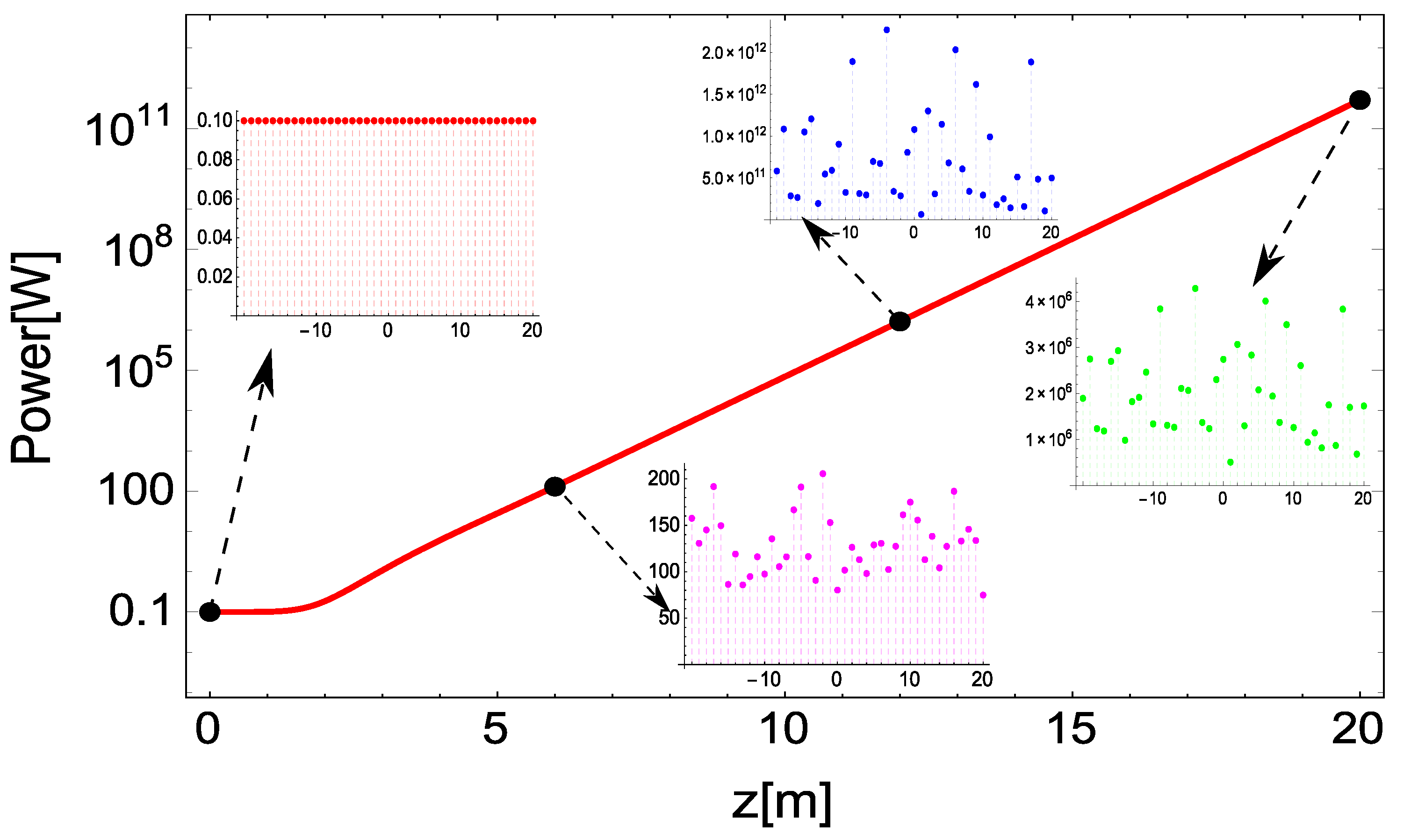
In the forthcoming section we apply the result obtained so far to the slice evolution.

5. Slice Evolution

The concept of slice phase space is a by-product of the S A S E F E L physics. It is indeed associated with the fact that, in these devices, the combination of mechanisms such as gain, slippage and finite coherence length, determines a local interaction, because the radiation experiences only a portion of the beam, having the longitudinal extension of a coherence length (see Figure 7 and Figure 8). The interaction is therefore sensitive to the slice-brightness, which is characterized by the relevant six dimensional phase space distribution [52,53,54,55,56,57,58].
The analysis associated with the transverse phase space and with the relevant electron-beam transport properties has already been accomplished in a number of papers, which have clarified a significant deal of the physical and practical issues regarding the evolution and interplay between slices and F E L power output and performances.
In this section we clarify the effect of longitudinal phase space, by the use of the formalism we outlined in the previous section. We sample the optical bunch as indicated in Figure 7 and characterize each slice with a progressive number [59,60].
Each slice is assumed to be Gaussian with an amount of charge Q s and an associated current
I s = Q s 2 π τ c , τ c L c c c o h e r e n c e t i m e .
A natural assumption is that the amount of charge follows the Gaussian shape of Figure 8, namely,
Q s = Q s * e ( s s * ) 2 δ 2 , δ = 2 π L c σ ζ
with δ 1 being the number of slices inside the bunch and s * representing the slice with largest current. With these assumptions we can write the slice Pierce parameter as
ρ s = ρ s * e ( s s * ) 2 δ 2 3 .
As we already stressed, each slice carries its own energy spread, and therefore we get a corresponding inhomogeneous parameter specified by
μ ˜ s = μ ˜ s * e ( s s * ) 2 δ 2 3 .
The energy spread corresponding to each slice may be completely random and that with largest current may carry the worst spread.
By taking into account these effects, we obtain the results reported in Figure 9 and Figure 10. The first refers to the case in which the slice with maximum current coincides with that at the center of the distribution, and the energy spread of each slice is chosen to be completely random. The second accounts for a configuration in which the maximum current is associated with a slice belonging to the rear part of the bunch.
Further comments including the elements for a more accurate computation of the slice distribution, are discussed in the forthcoming section dedicated to concluding remarks.

6. Final Remarks

This paper has treated different topics in the small signal evolution of high gain S A S E devices. We have just touched on the nonlinear effects leading to saturation. It has been underscored that the relevant pattern is accompanied by mechanisms of higher order bunching leading to the process of higher order harmonic emission.
From the phenomenological point of view, saturation can be included by modifying the small signal power evolution in Equation (29) as
I s ( z ˜ ) = I 0 A ( z ˜ ) 1 + I 0 I F A ( z ˜ ) 1 , I F = 2 ρ P E
where P E is the electron beam power intensity and I 0 is the input seed intensity. I 0 is usually specified by the rule of thumb that a value usually 10 8 below the saturated power density is chosen. The intensity I F yields the saturated power. The term at the denominator accounts for the saturation mechanisms, using a kind of logistic model, as displayed in Figure 11. The last figure needs its own mention: it shows the power growth in the deep saturated regime. Equation (63) reproduces well the evolution up the maximum and then remains fixed without following the oscillations (see Figure 12) due to the post saturation dynamics, characterized by e-beam rotation in phase-space, induced by an exchange of power between laser field and electrons.
A more complete view is reported in Figure 13. The physical content can be noted as reported below.
The figure exhibits the first and third harmonics, along with the associated wave packet evolution (upper and lower panels). We have assumed the growth from a coherent seed, and no spiking appears before the saturation. With the onset of the power oscillations, the optical packets start to be characterized by the appearance of side bands, which degrade the laser pulse itself in correspondence with the minima of the oscillations [61,62,63]. The effects of beam qualities can be also included by replacing A ( z ) with approximants discussed in the previous section.
The pivotal element of the discussion of this paper has been centered around the F E L high gain equation, which, including the necessary modifications, is able to describe different physical situations regarding the F E L phenomenology. The F E L high gain equation has been derived from the F E L pendulum equation after a suitable linearization. A different treatment can be, however, exploited: it employs a Hamiltonian picture and the associated Liouville equation. The by-product of this treatment (see, e.g., [9,10,17,18,49,50,52,53,54,55,56,57,58,59,60,64]) yields results not dissimilar from those discussed in the previous sections, and the bunching coefficient of the n-th harmonic induced by the fundamental behaves like a n . Such an effect is of fundamental importance in the handling of the so-called segmented magnet configurations [50,65]. F E L adopting this type of solution exploits the growth of the bunching inside a first section, which is interrupted and connected to a second undulator, tuned at one of its harmonics. The result is the growth of a coherent signal emerging from the beam bunching acquired in the first section. Methods based on the joint use of the solution of the high gain F E L equation, on the study of the relevant Liouville equation and on the use of massive simulation codes, allow the possibility of deriving useful scaling relations concerning the onset and saturation of the F E L signal from a suitably pre-bunched beam [65].
Π n ( z ) = Π 0 , n e z L g ( n ) 1 + Π 0 , n Π F , n e z L g ( n ) 1 , L g ( n ) = L g n , Π 0 , n = c n P 0 9 ρ P E n Π F , n , Π F , n = 1 n f b , n n f b , 1 2 P F
where the coefficients c n are just numerical characteristics for each harmonic. Equation (64) yields the growth of the nonlinear part of the n-th harmonic. The relevant gain length is decreased by a factor corresponding to the order of the harmonics; Π F , n is the harmonic saturated power. The number of photons/seconds at the n-th harmonic can accordingly be calculated as
N ˙ n = Π F , n n ħ ω = E n N ˙ 1 , E n = 1 n n f b , n n f b , 1 2 ,
where E n represents a kind of efficiency displaying how the fundamental harmonic contributes to the higher order harmonics.
We have so far given a general discussion of analytical and numerical methods to treat the F E L intensity evolution in the high gain/ S A S E regime. We have just touched on the problems associated with short pulse effects, which will be treated elsewhere in a dedicated monography.

Author Contributions

Conceptualization, G.D., E.D.P., E.S.; methodology, G.D., E.D.P., E.S. software, E.D.P., E.S.; validation, G.D., E.D.P., S.L., E.S.; formal analysis, G.D., E.D.P., S.L., E.S.; data curation, G.D., E.D.P., S.L., E.S. writing–original draft preparation, G.D., E.D.P., E.S.; writing–review and editing, S.L.; visualization, G.D., E.D.P., S.L., E.S. supervision, G.D., E.D.P., S.L., E.S.; project administration, E.D.P. All authors have read and agreed to the published version of the manuscript.

Funding

This research received no external funding.

Acknowledgments

The work of S. Licciardi was supported by an Enea Research Center individual fellowship.

Conflicts of Interest

The authors declare no conflict of interest.

References

  1. Madey, J.M.J. Stimulated Emission of Bremsstrahlung in a Periodic Magnetic Field. J. Appl. Phys. 1971, 42, 1906. [Google Scholar] [CrossRef]
  2. Dattoli, G.; Di Palma, E.; Pagnutti, S.; Sabia, E. Free Electron coherent sources: From microwave to X-rays. Phys. Rep. 2018, 739, 1–51. [Google Scholar] [CrossRef]
  3. Neyman, P.J.; Colson, W.B.; Gottschalk, S.C.; Todd, A.M.M.; Blau, J.; Cohn, K. Free Electron Lasers in 2017. In Proceedings of the 38th International Free Electron Laser Conference, FEL2017, Santa Fe, NM, USA, 20–25 August 2017; Available online: https://accelconf.web.cern.ch/fel2017/papers/mop066.pdf (accessed on 17 December 2020).
  4. Rossbach, J.; Schneider, J.R.; Wurth, W. 10 years of pioneering X-ray science at the Free-Electron Laser FLASH at DESY. Phys. Rep. 2019, 808, 1–74. [Google Scholar] [CrossRef]
  5. Topics. Available online: https://lcls.slac.stanford.edu/ (accessed on 17 December 2020).
  6. Topics. Available online: https://www.elettra.trieste.it/lightsources/fermi/machine.html (accessed on 17 December 2020).
  7. Topics. Available online: http://xfel.riken.jp/eng/ (accessed on 17 December 2020).
  8. Colson, W.B. Free Electron Laser Theory. Ph.D. Thesis, Stanford University, Stanford, CA, USA, 1977. [Google Scholar]
  9. Colson, W.B. Classical Free Electron Laser Theory, Laser Handbook; Colson, W.B., Pellegrini, C., Renieri, A., Eds.; North-Holland: Amsterdam, The Netherlands, 1990; Volume VI. [Google Scholar]
  10. Saldin, E.L.; Schneidmiller, E.V.; Yurkov, M.V. The Physics of Free Electron Lasers; Springer: Berlin/Heidelberg, Germany, 2000. [Google Scholar] [CrossRef]
  11. Kim, K.J.; Huang, Z.; Lindberg, R. Synchrotron Radiation and Free Electron Lasers; Cambridge University Press: Cambridge, UK, 2017. [Google Scholar] [CrossRef]
  12. Bergmann, U.; Yachandra, V.; Yano, J. X-ray Free Electron Laser: Applications in Materials, Chemistry and Biology; Royal Society of Chemistry: Cambridge, UK, 2017; ISBN 978-1-84973-100-3. [Google Scholar]
  13. Dattoli, G.; Doria, A.; Sabia, E.; Artioli, M. Charged Beam Dynamics, Particle Accelerators and Free Electron Lasers; IOP Publishing Ltd.: Bristol, UK, 2017. [Google Scholar]
  14. Szarmes, E.B. Classical Theory of Free-Electron Lasers; IOP Publishing Ltd.: Bristol, UK, 2017. [Google Scholar]
  15. Jaeschke, E.; Khan, S.; Schneider, J.R.; Hastings, J.B. Synchrotron Light Sources and Free-Electron Lasers; Springer: Berlin/Heidelberg, Germany, 2016; ISBN 978-3-319-14393-4. [Google Scholar]
  16. Behrens, C.; Schmüser, P.; Dohlus, M.; Rossbach, J. Free-Electron Lasers in the Ultraviolet and X-ray Regime; Springer: Berlin/Heidelberg, Germany, 2014. [Google Scholar]
  17. Dattoli, G.; Ottaviani, P.L. Fel Small Signal Dynamics and Electron Beam Prebunching; ENEA Internal Report, RT/INN/93/10; ENEA: Frascati, Italy, 1993. [Google Scholar]
  18. Dattoli, G.; Ottaviani, P.L.; Pagnutti, S. Booklet for FEL Design: A Collection of Practical Formulae; ENEA—Edizioni Scientifiche: Frascati, Italy, 2007. [Google Scholar]
  19. Bonifacio, R.; Pellegrini, C.; Narducci, L.M. Collective instabilities and high-gain regime in a free electron laser. Opt. Commun. 1984, 50, 373–378. [Google Scholar] [CrossRef] [Green Version]
  20. Haus, H. Quantum Electronics, Noise in Free Electron Laser Amplifier. IEEE J. Quantum Electron. 1981, 17, 1427–1435. [Google Scholar] [CrossRef]
  21. Dattoli, G.; Marino, A.; Renieri, A.; Romanelli, F. Progress in the Hamiltonian picture of the free-electron laser. IEEE J. Quantum Electron. 1981, 17, 1371–1387. [Google Scholar] [CrossRef]
  22. Petelin, M.I. On the theory of ultrarelativistic cyclotron self-resonance masers. Radiophys. Quantum Electron. 1974, 17, 686–690. [Google Scholar] [CrossRef]
  23. Nusinovich, G. Introduction to the Physics of Gyrotrons; The John Hopkins University Press: Baltimore, MD, USA, 2004. [Google Scholar]
  24. Bratman, V.L.; Ginzburg, N.S.; Petelin, M.I. Common properties of free electron lasers. Opt. Commun. 1979, 30, 409–412. [Google Scholar] [CrossRef]
  25. Di Palma, E.; Sabia, E.; Dattoli, G.; Licciardi, S.; Spassovsky, I. Cyclotron auto resonance maser and free electron laser devices: A unified point of view. J. Plasma Phys. 2017, 83, 905830102. [Google Scholar] [CrossRef]
  26. Caloi, R.; Ciocci, F.; Dattoli, G.; Torre, A. The High-Gain FEL Equation: An Inexpensive Numerical Algorithm. Il Nuovo Cimento B 1991, 106, 627–640. [Google Scholar] [CrossRef]
  27. Dattoli, G.; Renieri, A.; Torre, A. Lecture on Free Electron Laser Theory and Related Topics; World Scientific: Singapore, 1990. [Google Scholar]
  28. Tremaine, A.J.; Rosenzweig, B.; Anderson, S.; Frigola, P.; Hogan, M.; Murokh, A.; Pellegrini, C.; Nguyen, D.C.; Sheffield, R.L. Observation of Self-Amplified Spontaneous-Emission-Induced Electron-Beam Microbunching Using Coherent Transition Radiation. Phys. Rev. Lett. 1998, 81, 5816. [Google Scholar] [CrossRef] [Green Version]
  29. Nguyen, D.C.; Sheffield, R.L.; Fortgang, C.M.; Kinross-Wright, J.M.; Ebrahim, N.A.; Goldstein, J.C. A High-Power compact Regenerative Amplifier FEL. In Proceedings of the 17th PAC Conference, Vancouver, BC, Canada, 12–16 May 1997; p. 897. Available online: https://cds.cern.ch/record/909415?ln=it (accessed on 17 December 1997).
  30. Dattoli, G.; Cabrini, S.; Giannessi, L. Simple Model of Gain Saturation in Free Electron Laser. Phys. Rev. A 1991, 44, 8433. [Google Scholar] [CrossRef] [PubMed]
  31. Dattoli, G. Logistic function and evolution of free-electron-laser oscillators. J. Appl. Phys. 1998, 84, 2393–2398. [Google Scholar] [CrossRef]
  32. Dattoli, G.; Ottaviani, P.L. Semi-analytical models of Free Electron Laser Saturation. Opt. Comm. 2002, 204, 283–297. [Google Scholar] [CrossRef]
  33. Dattoli, G.; Giannessi, L.; Ottaviani, P.L.; Ronsivalle, C. Semi-analytical model of self-amplified spontaneous-emission free-electron lasers, including diffraction and pulse-propagation effects. J. Appl. Phys. 2004, 95, 3206–3210. [Google Scholar] [CrossRef]
  34. Shih, C.C.; Yariv, A. Inclusion of Space-Charge Effects with Maxwell’s Equations in the Single-Particle Analysis of Free-Electron Lasers. IEEE J. Quantum Electron. 1981, 17, 1387–1394. [Google Scholar] [CrossRef] [Green Version]
  35. Dattoli, G.; Torre, A.; Centioli, C.; Richetta, M. Free Electron Laser Operation in the Intermediate Gain Region. IEEE J. Quantum Electron. 1989, 25, 2327–2331. [Google Scholar] [CrossRef]
  36. Elias, L.R.; Fairbank, W.M.; Madey, J.M.J.; Schwettman, H.A.; Smith, T.I. Observation of Stimulated Emission of Radiation by Relativistic Electrons in a Spatially Periodic Transverse Magnetic Field. Phys. Rev. Lett. 1976, 36, 717. [Google Scholar] [CrossRef] [Green Version]
  37. Deacon, D.A.G.; Elias, L.R.; Madey, J.M.J.; Ramian, G.J.; Schwettman, H.A.; Smith, T.I. First Operation of a Free-Electron Laser. Phys. Rev. Lett. 1977, 38, 892–894. [Google Scholar] [CrossRef]
  38. Colson, W.B. The nonlinear wave equation for higher harmonics in free-electron lasers. IEEE J. Quantum Electron. 1981, 17, 1417–1427. [Google Scholar] [CrossRef]
  39. Dattoli, G.; Ottaviani, P.L.; Pagnutti, S. Non Linear Harmonic Generation in high gain free electron laser. J. Appl. Phys. 2005, 97, 113102. [Google Scholar] [CrossRef]
  40. Dattoli, G.; Ottaviani, P.L.; Pagnutti, S. The PROMETEO Code: A flexible tool for Free Electron Laser study. Il Nuovo Cimento C 2009, 32, 283–287. [Google Scholar]
  41. Gallardo, J.C.; Elias, L.R.; Dattoli, G.; Renieri, A. Integral equation for the laser field in a long-pulse free-electron laser. Phys. Rev. A 1987, 36, 3222. [Google Scholar] [CrossRef]
  42. Colson, W.B.; Dattoli, G.; Ciocci, F. Angular-gain spectrum of free-electron lasers. Phys. Rev. A 1985, 31, 828. [Google Scholar] [CrossRef]
  43. Giannessi, L. Seeding and Harmonic Generation in Free-Electron Lasers. In Synchrotron Light Sources and Free-Electron Lasers; Springer: Berlin/Heidelberg, Germany, 2016; pp. 195–223. ISBN 978-3-319-14393-4. [Google Scholar]
  44. Lambert, G.; Hara, T.; Garzella, D.; Tanikawa, T.; Labat, M.; Carre, B.; Kitamura, H.; Shintake, T.; Bougeard, M.; Inoue, S.; et al. Injection of harmonics generated in gas in a free electron laser providing intense and coherent extreme-ultraviolet light. Nat. Phys. 2008, 4, 296–300. [Google Scholar] [CrossRef]
  45. Colson, W.B.; Gallardo, J.C.; Bosco, P.M. Free-electron-laser gain degradation and electron-beam quality. Phys. Rev. A 1986, 34, 4875. [Google Scholar] [CrossRef]
  46. Dattoli, G.; Ottaviani, P.L.; Segreto, A.; Altobelli, G. Free electron laser gain: Approximant forms and inclusion of inhomogeneous broadening contributions. J. Appl. Phys. 1995, 77, 6162. [Google Scholar] [CrossRef]
  47. Dattoli, G.; Giannessi, L.; Torre, A.; Segreto, A. The pulse propagation problem in free electron lasers: Gain parametrization formulae. J. Appl. Phys. 1996, 79, 6729. [Google Scholar] [CrossRef]
  48. Bonifacio, R.; McNeil, B.W.J.; Pierini, P. Superradiance in the high-gain free-electron laser. Phys. Rev. A 1989, 40, 4467. [Google Scholar] [CrossRef]
  49. Saldin, E.L.; Schneidmiller, E.A.; Yurkov, M.V. Diffraction effects in the self-amplified spontaneous emission FEL. Opt. Commun. 2000, 186, 185–209. [Google Scholar] [CrossRef]
  50. Saldin, E.L.; Schneidmiller, E.A.; Yurkov, M.V. Properties of the third harmonic of the radiation from self-amplified spontaneous emission free electron laser. Phys. Rev. Spec. Top. Accel. Beams 2006, 9, 030702. [Google Scholar] [CrossRef] [Green Version]
  51. Dattoli, G.; Sabia, E.; Ottaviani, P.L.; Pagnutti, S.; Petrillo, V. Longitudinal dynamics of high gain free electron laser amplifiers. Phys. Rev.Spec. Top. Accel. Beams 2013, 16, 030704. [Google Scholar] [CrossRef]
  52. Merminga, L.; Morton, P.L.; Seeman, J.; Spence, W.L. Transverse phase space in the presence of dispersion. In Proceedings of the 1991 Institute of Electrical and Electronics Engineers (IEEE) Particle Accelerator Conference (PAC), San Francisco, CA, USA, 6–9 May 1991; Volume 910506, pp. 461–463. [Google Scholar]
  53. Dowell, D.H.; Bolton, P.R.; Clendenin, J.E.; Emma, P.; Gierman, S.M.; Graves, W.S.; Limborg, C.G.; Murphy, B.F.; Schmerge, J.F. Slice emittance measurements at the SLAC Gun Test Facility. Nucl. Instrum. Meth. A 2003, 507, 327–330. [Google Scholar] [CrossRef] [Green Version]
  54. Ferrario, M.; Alesini, D.; Bellaveglia, M.; Benfatto, M.; Boni, R.; Boscolo, M.; Castellano, M.; Chiadroni, E.; Clozza, A.; Cultrera, L.; et al. Recent results of the SPARC FEL experiments. In Proceedings of the 31st FEL Conference Liverpool, Liverpool, UK, 23–28 August 2009. [Google Scholar]
  55. Bettoni, S.; Aiba, M.; Beutner, B.; Pedrozzi, M.; Prat, E.; Reiche, S.; Schietinger, T. Preservation of low slice emittance in bunch compressors. Phys. Rev. Accel. Beams 2016, 19, 034402. [Google Scholar] [CrossRef] [Green Version]
  56. Dattoli, G.; Giannessi, L.; Torre, A. Unified view of free-electron laser dynamics and of higher-harmonics electron bunching. J. Opt. Soc. Am. 1993, 10, 2136–2143. [Google Scholar] [CrossRef]
  57. Dattoli, G.; Giannessi, L.; Ottaviani, P.L. Free electron laser small signal dynamics and inclusion of electron-beam energy phase correlation. J. Appl. Phys. 1999, 86, 1710–1715. [Google Scholar] [CrossRef]
  58. Dattoli, G.; Giannessi, L.; Ottaviani, P.L.; Pagnutti, S. Energy Phase Correlation and Pulse Dynamics in Short Bunch High Gain FELs. Opt. Commun. 2010, 285, 710–714. [Google Scholar] [CrossRef] [Green Version]
  59. Dattoli, G.; Sabia, E.; Ronsivalle, C.; Del Franco, M.; Petralia, A. Slice emittance, projected emittance and properties of the SASE FEL radiation. Nucl. Instrum. Methods Phys. Res. Sect. A Accel. Spectrometers Detect. Assoc. Equip. 2012, 671, 51–61. [Google Scholar] [CrossRef]
  60. Bonifacio, R.; De Salvo, L.; Pierini, P. Large harmonic bunching in a high-gain free-electron laser. Nucl. Instrum. Methods Phys. Res. Sect. A Accel. Spectrometers Detect. Assoc. Equip. 1990, 293, 627–629. [Google Scholar] [CrossRef]
  61. Dattoli, G.; Ottaviani, P.L.; Pagnutti, S. High gain amplifiers: Power oscillations and harmonic generation. J. Appl. Phys. 2007, 102, 033103. [Google Scholar] [CrossRef]
  62. Giannessi, L.; Musumeci, P.; Spampinati, S. Nonlinear pulse evolution in seeded free-electron laser amplifiers and in free-electron laser cascades. J. Appl. Phys. 2005, 98, 043110. [Google Scholar] [CrossRef]
  63. Yang, X.; Mirian, N.; Giannessi, L. Postsaturation dynamics and superluminal propagation of a superradiant spike in a free-electron laser amplifier. Phys. Rev. Accel. Beams 2020, 23, 010703. [Google Scholar] [CrossRef] [Green Version]
  64. Gardelle, J.; Labrouche, J.; Marchese, G.; Rullier, J.L.; Villate, D. Analysis of the beam bunching produced by a free electron laser. Phys. Plasmas 1996, 3, 4197. [Google Scholar] [CrossRef]
  65. Dattoli, G.; Ottaviani, P.L.; Pagnutti, S. Theory of High Gain Free Electron Laser, operating with segmented undulators. J. Appl. Phys. 2006, 99, 044907. [Google Scholar] [CrossRef]
Figure 1. Square modulus of the dimensionless amplitude vs. the detuning parameter for g 0 = 0.5 and different values of τ : ( 0.5 , 0.6 , 0.7 , 0.8 , 0.9 , 1 ) . The intensity grows with incresing dimensionless time.
Applsci 11 00085 g001
Figure 2. Intensity vs. detuning ν0 and dimensionless time τ.
Applsci 11 00085 g002
Figure 3. Comparison between Equation (29) and the pure exponential behavior for L g = 0.4 .
Applsci 11 00085 g003
Figure 4. Power density (a.u.) vs. z and gain function “measured“ at different points inside the undulator. Above the last point, where the dotted curve starts, the small signal gain is not properly defined because the small signal approximation does not strictly apply. The curves have been derived for the parameters ρ 0 = 6.8 · 10 4 and λ u = 5 cm. The small signal gain coefficient goes from 5.35 · 10 3 to 5.35 .
Applsci 11 00085 g004
Figure 5. Harmonic evolution and nonlinear harmonic generation which is triggered after the dashed line, where the bunching effects become significant.
Applsci 11 00085 g005
Figure 6. Intensity vs. z ˜ , ν ˜ for inhomogeneous parameters μ ˜ ε = 1 , g 0 = 100 , a 0 = 1 .
Applsci 11 00085 g006
Figure 7. Slice number sampling and shape, using the e-bunch distribution as the reference frame.
Applsci 11 00085 g007
Figure 8. Bunched envelope, associated slices and superimposed radiation.
Applsci 11 00085 g008
Figure 9. Slice evolution inside the undulator at different Z; the energy spread has been randomly chosen and the current follows the bunch Gaussian distribution with s = 0 , λ u = 0.02 , ρ 0 = 0.001 , μ ε = 0.0004 and ν = 0 . The initial distribution z = 0 of the slices is the same as in Figure 8. The vertical axis is in log-scale; the insets are plotted in linear scale.
Applsci 11 00085 g009
Figure 10. Same as Figure 9—all slices with the same energy spread and the maximum current associated with the rear part of the bunch ( s = 1 ). Slice evolution vs z and intensity evolution vs. z. The slices are characterized by the same amount of charge and different values of the energy spread with λ u = 0.015 , ρ 0 = 0.0011 , σ ε = 0.05 , σ d = 0.002 , δ = 0.01 and I 0 = 10 1 . The intensity growth does not refer to a single slice but to the relevant average. The slices have a flat distribution in z, and each is characterized by an initial seed of 0.1 W. The vertical axis is in log-scale; the insets are plotted in linear scale.
Applsci 11 00085 g010
Figure 11. Same parameters as in Figure 10 with the inclusion of the saturation. The slices have a flat distribution in z, and each is characterized by an initial seed of 0.1 W. The vertical axis is in log-scale; the insets are plotted in linear scale.
Applsci 11 00085 g011
Figure 12. Power growth and oscillation after saturation (no specific parameters of the simulation have been inserted because we are just interested to the oscillating behavior, characterizing any S A S E F E L operating with constant parameters).
Applsci 11 00085 g012
Figure 13. First and third harmonic power growth vs. z, along with the power oscillations and associated changes in the laser packet distribution.
Applsci 11 00085 g013
Publisher’s Note: MDPI stays neutral with regard to jurisdictional claims in published maps and institutional affiliations.

