A Data-Driven Approach of Takagi-Sugeno Fuzzy Control of Unknown Nonlinear Systems

Abstract

A novel approach to build a Takagi-Sugeno (T-S) fuzzy model of an unknown nonlinear system from experimental data is presented in the paper. The neuro-fuzzy models or, more specifically, fuzzy basis function networks (FBFNs) are trained from input–output data to approximate the nonlinear systems for which analytical mathematical models are not available. Then, the T-S fuzzy models are derived from the direct linearization of the neuro-fuzzy models. The operating points for linearization are chosen using the evolutionary strategy to minimize the global approximation error so that the T-S fuzzy models can closely approximate the original unknown nonlinear system with a reduced number of linearizations. Based on T-S fuzzy models, optimal controllers are designed and implemented for a nonlinear two-link flexible joint robot, which demonstrates the possibility of implementing the well-established model-based optimal control method onto unknown nonlinear dynamic systems.

1. Introduction

The Takagi-Sugeno (T-S) fuzzy model is a powerful and practical engineering tool for modeling and control of complex nonlinear systems. It proves to be a universal function approximator that can approximate any smooth nonlinear functions to any degree of accuracy [1,2] and is less sensitive to the curse of dimensionality than other fuzzy models [3]. The concept of T-S fuzzy model is similar to the piecewise linear approximation approaches in nonlinear control, which linearizes a system at a set of selected operating points and designs a local linear feedback controller for each linear model. However, since the overall control action is switching among the local linear controllers according to system states and thus there is only one local controller active at a certain time in such approaches, it can only ensure the stability and performance of the control system at the neighborhood of selected operating points [4], In contrast, the T-S fuzzy model approximates the entire nonlinear system by fuzzy inference among local linear models so that the overall control action can be generated by aggregation of local linear control laws [5]. Therefore, it empowers a paradigm of designing controllers for local linear models while analyzing stability for the global nonlinear system [6]. The T-S fuzzy-model-based control that blends feedback controllers from local models is referred to as Parallel Distributed Compensation (PDC) scheme, in which the stability of the overall control system is assessed through Lyapunov stability analysis, especially by the Linear Matrix Inequality (LMI) technique [7,8,9,10,11,12].

To take advantage of T-S fuzzy-model-based control, the identification of T-S fuzzy model has attracted great research interest. There are two kinds of methods for establishing T-S fuzzy models. One is linearizing the original system at a series of operating points when an analytical model of the system is available. The other is the consecutive structure and parameter identification from the data generated by the unknown system [6], which is more of interest to us. The structure identification refers to the selection of locations of fuzzy rules based on clustering [13,14]. With the determined antecedent structural parameters, the T-S fuzzy model transforms into a set of linear models, of which the parameters are obtained by the recursive least square method [15,16], genetic algorithm [17] or particle swarm optimization [18]. The objective of data-driven approaches is to minimize the global prediction error of a T-S fuzzy model. However, they may result in constituent linear models significantly different from the local linearization of nonlinear systems, though they may offer good global performance [19]. Hence, the T-S models obtained by these methods might not be satisfactory for the controller design in the Parallel Distributed Compensation (PDC) scheme, since the local compensators need to be designed based on local linear models.

The authors in [2] studied various identification algorithms and concluded that the constrained and regularized identification method can improve the interpretability of constituent local models as local linearization, and the locally weighted least square technique may facilitate the compromise between the local and global accuracy of T-S models. However, the effectiveness and practicality of this method were demonstrated only by very simple examples. When considering more complicated higher-order and multivariate problems, the issues related to interpretability and identifiability will be more pronounced and difficult to address.

An alternative method to circumvent these difficulties is presented in this paper. A neuro-fuzzy model referred to as fuzzy basis function networks (FBFN) is adopted to approximate the unknown nonlinear systems [20]. The Stone–Weierstrass theorem proves that this kind of neuro-fuzzy model could approximate any real continuous function on a compact domain arbitrarily well [21]. Then, the T-S fuzzy model is derived from the linearization of the neuro-fuzzy model at a series of operating points. Therefore, each local model is close to the local linearization of the original system and, thus, suitable for local compensator design. In addition, the positions of operating points for linearization are optimized by the evolutionary strategy to minimize global approximation error so that the entire T-S fuzzy model is a good global approximation of the original system. A fuzzy control scheme can be applied to the consequent T-S fuzzy model in which a local optimal compensator is designed for each of the local affine models and the overall control action is derived from the fuzzy inferencing of local control actions. The contribution of this paper is that it presents a practical way to build T-S fuzzy models with both good local and global approximations by deriving the direct linearization of FBFN models and introducing the evolutionary strategy for fuzzy rule location selection. Compared with the existing methods, the method proposed in this paper is less involved compared with nonlinear controllers while the performance is not compromised and, thus, it is particularly suitable for controller design of complex unmodeled nonlinear systems in practice.

This paper is organized as follows: Section 2 presents the structure of the T-S fuzzy model; Section 3 elaborates the proposed T-S fuzzy model identification approach; Section 4 explains the design of fuzzy optimal controller; Section 5 demonstrates an example of T-S model identification and optimal control of a robotic system; Section 6 concludes the paper.

2. Takagi-Sugeno Fuzzy Model

T-S fuzzy models represent complicated multi-input-multi-output (MIMO) systems with fuzzy inference rules and local linear models as follows:

$${\mathit{R}}^{\mathit{k}}: \mathrm{IF} z_1 \mathrm{is} {{\mathit{F}}_{\mathbf{1}}}^{\mathit{k}}, \cdots , z_{\mathrm{v}}\mathrm{is} {{\mathit{F}}_{\mathit{v}}}^{\mathit{k}}, \mathrm{THEN} \dot{x}=A_{k}x\left(t\right)+B_{k}u\left(t\right)+d_k,$$

where R^k denotes the kth fuzzy rule, k ∈ {1, 2, ⋯, p}, p is the number of fuzzy rules, F_j^k (j = 1, 2, ⋯, v) are the input fuzzy sets, x(t) ∈ Rⁿ is the state variable vector, u(t) ∈ R^m is the input variable vector, z(t): = [z₁, z₂, ⋯, z_v] are a subset of measurable or observable variables in the state and input vectors that are used for fuzzification, and (A_k, B_k, d_k) are the matrices of the kth local model [6]. If the constant bias vector is not null, d_k ≠ 0, for some fuzzy inference rules, the corresponding local models are affine models instead of linear models.

By using the product fuzzy inference, singleton output membership functions, and centroid defuzzifier, a T-S fuzzy model in continuous-time state-space form can be organized as:

$$\dot{x}=A\left(\mu \right)x\left(t\right)+B\left(\mu \right)u\left(t\right)+d\left(\mu \right),$$

(1)

where $A\left(\mu \right)={\displaystyle {\sum }_{k=1}^p{\mu }_k{A}_k}$, $B\left(\mu \right)={\displaystyle {\sum }_{k=1}^p{\mu }_k{B}_k}$, $d\left(\mu \right)={\displaystyle {\sum }_{k=1}^p{\mu }_k{d}_k}$ and µ_k denotes the normalized fuzzy membership function ${\mu }_k={\xi }^k\left(z\right)/{\displaystyle {\sum }_{k=1}^p{\xi }^k\left(z\right)}$ with ${\xi }^k\left(z\right)={\displaystyle {\prod }_{i=1}^v{\Phi }_i^k\left(z_i\right)}$. ${\Phi }_i^k\left(z_i\right)$ represents the i-th membership function in fuzzy set F_i^k of the k-th fuzzy rule. Due to the fact that the membership functions are nonlinear (e.g., triangular or Gaussian), the model in Equation (1), as an aggregation of local linear or affine models, is also a nonlinear model in nature.

3. Identification of Takagi-Sugeno Fuzzy Model

The T-S fuzzy model is expected to attain a good approximation of not only the local dynamics of the underlying system to facilitate local compensator design, but also the global dynamics to guarantee the overall control performance. However, considering them together is difficult because building constituent local linear models from input-output data is not always straightforward and the tradeoff between the local and global accuracy should be carefully addressed [2].

In this paper, a novel approach that utilizes the neuro-fuzzy model to obtain a T-S fuzzy model is proposed. The neuro-fuzzy models are based on the fusion of fuzzy inference systems and neural networks. Among diverse neuro-fuzzy models, the one proposed by Wang and Mendel [20], which is also known as fuzzy basis function network (FBFN), has gained much attention as it has a similar structure to radial basis function networks (RBFNs) and thus can adopt the training methods that are already established for the RBFN. It has been proved that the FBFNs can uniformly approximate any real continuous nonlinear functions on a compact set to arbitrary accuracy [21].

First, from the input-output data, a set of multi-input-single-output FBFNs with product fuzzy inference, Gaussian membership functions (MFs), and centroid defuzzifier are trained by the least square algorithm [22] to approximate the nonlinear system whose analytical mathematical model is not available. Each FBFN can be represented as a fuzzy system in layered network form (see Figure 1), and is used to approximate the dynamics of one state variable. For example, the FBFN for the p-th state variable is constructed using fuzzy rules as:

$${{\mathit{R}}_p}^l: \mathrm{IF} x_1 \mathrm{is} {{\mathit{A}}_{1p}}^l, \cdots , x_n\mathrm{is} {{\mathit{A}}_{np}}^l \mathrm{and} u_1 \mathrm{is} {{\mathit{B}}_{1p}}^l, \cdots , u_m \mathrm{is} {{\mathit{B}}_{mp}}^l, \mathrm{THEN}{\dot{x}}_p=w_p^l,$$

where l ∈ {1, 2, ⋯, M_p}, and Mp is the number of fuzzy rules for the p-th FBFN. Through fuzzy inference and defuzzification, the FBFN based on the above fuzzy rules can be written as:

$$\begin{array}{cc}{\dot{x}}_p=f_p\left(x,u\right)=\frac{{\displaystyle \sum _{l=1}^{M_p}{w}_p{}^l{\displaystyle \prod _{i=1}^n{e}^{-\frac{1}{2}{\left(\frac{x_i-x_{ip}^l}{{\sigma }_{ip}^l}\right)}^2}}{\displaystyle \prod _{j=1}^m{e}^{-\frac{1}{2}{\left(\frac{u_j-u_{jp}^l}{{\sigma }_{ujp}^l}\right)}^2}}}}{{\displaystyle \sum _{l=1}^{M_p}{\displaystyle \prod _{i=1}^n{e}^{-\frac{1}{2}{\left(\frac{x_i-x_{ip}^l}{{\sigma }_{ip}^l}\right)}^2}}{\displaystyle \prod _{j=1}^m{e}^{-\frac{1}{2}{\left(\frac{u_j-u_{jp}^l}{{\sigma }_{ujp}^l}\right)}^2}}}}& p=1,2,\cdots ,n\end{array},$$

(2)

where x: = [x₁, x₂, ⋯, x_n] is the state variable vector, u: = [u₁, u₂, ⋯, u_m] is the input vector, and w_p^l is the weighting factor. The x_ip^l and σ_ip^l are the centers and widths of Gaussian MFs $e^{-\frac{1}{2}{\left(\frac{x_i-x_{ip}^l}{{\sigma }_{ip}^l}\right)}^2}$ in fuzzy set A_ip^l, and the u_ip^l and σ_uip^l are the centers and widths of Gaussian MFs $e^{-\frac{1}{2}{\left(\frac{x_i-x_{ip}^l}{{\sigma }_{ip}^l}\right)}^2}$ in fuzzy set B_ip^l.

Next, the T-S fuzzy model is derived from the neuro-fuzzy model by linearizing Equation (2). Linearization about an operating point (x_k, u_k) results in

$$\dot{x}=A_k\left(x-x_k\right)+B_k\left(u-u_k\right)+f\left(x_k,u_k\right)+H.O.T,$$

(3)

where H.O.T denotes the higher order terms in the local model, which will be neglected in the following analysis, $f\left(x_k,u_k\right)={\left[f_1\left(x_k,u_k\right),\dots ,f_n\left(x_k,u_k\right)\right]}^T$, and

$$A_k={\left[\begin{array}{ccc}\frac{\partial f_1\left(x,u\right)}{\partial x_1}& \cdots & \frac{\partial f_1\left(x,u\right)}{\partial x_n}\\ ⋮& \ddots & ⋮\\ \frac{\partial f_n\left(x,u\right)}{\partial x_1}& \cdots & \frac{\partial f_n\left(x,u\right)}{\partial x_n}\end{array}\right]}_{x=x_k,u=u_k},$$

(4)

By taking the partial derivative of Equation (2) with respect to x_q, one can get

$$\frac{\partial f_p\left(x,u\right)}{\partial x_q}=\frac{{\displaystyle \sum _{l=1}^{M_p}{w}_p{}^l{a}_p^l{\displaystyle \sum _{l=1}^{M_p}{a}_p^l{q}_p^l}}-{\displaystyle \sum _{l=1}^{M_p}{a}_p^l}{\displaystyle \sum _{l=1}^{M_p}{w}_p{}^l{a}_p^l{q}_p^l}}{{\left({\displaystyle \sum _{l=1}^{M_p}{a}_p^l}\right)}^2},$$

(5)

where

$$\begin{array}{l}{a}_p^l={\displaystyle \prod _{i=1}^n{e}^{-\frac{1}{2}{\left(\frac{x_i\left(k\right)-x_{ip}^l}{{\sigma }_{ip}^l}\right)}^2}}{\displaystyle \prod _{j=1}^m{e}^{-\frac{1}{2}{\left(\frac{u_j\left(k\right)-u_{jp}^l}{{\sigma }_{ujp}^l}\right)}^2}}\\ q_p^l=\frac{x_q\left(k\right)-x_{qp}^l}{{\left({\sigma }_{qp}^l\right)}^2}\end{array}$$

(6)

Similarly,

$$B_k={\left[\begin{array}{ccc}\frac{\partial f_1\left(x,u\right)}{\partial u_1}& \cdots & \frac{\partial f_1\left(x,u\right)}{\partial u_m}\\ ⋮& \ddots & ⋮\\ \frac{\partial f_n\left(x,u\right)}{\partial u_1}& \cdots & \frac{\partial f_n\left(x,u\right)}{\partial u_m}\end{array}\right]}_{x=x_k,u=u_k},$$

(7)

where $\partial f_p\left(x,u\right)/\partial u_q$ has the same expression as Equation (5) except that:

$$q_p^l=\frac{u_q\left(k\right)-u_{qp}^l}{{\left({\sigma }_{uqp}^l\right)}^2}$$

(8)

For simplicity, and also by neglecting the higher-order terms, Equation (3) can be rewritten as

$$\dot{x}=A_{k}x+B_{k}u+d_k,$$

(9)

where

$$d_k=f\left(x_k,u_k\right)-A_k{x}_k-B_k{u}_k.$$

(10)

The affine term d_k is non-null, i.e., d_k ≠ 0 in general even if the operating point is an equilibrium point other than the origin [23]. Including the affine terms will offer a more accurate local approximation of the system’s dynamics around the operating points.

Then, the operating points used for linearization need to be chosen carefully to achieve a good global approximation of the original system. Meanwhile, it is desirable to minimize the number of linearization so that the number of fuzzy rules in the T-S fuzzy model can be reduced and the fuzzy controller synthesized in the following section will be more computationally efficient. To reduce the number of linearization points, it is necessary to know which variables among z = [z₁, z₂, ⋯, z_v] in fuzzy inference are the major sources of nonlinearity. These variables should be assigned more positions while the variables that are minor sources can be assigned fewer positions. A measure to roughly recognize the source of nonlinearity by inspecting the variation of linearized A-matrix is presented in Section 5. If the i-th variable z_i is to be assigned p_i positions {z_i,1, …, z_i,pi}, then by combination of the ${\displaystyle {\sum }_{i=1}^v{p}_i}$ positions, there will be $p={\displaystyle {\prod }_{i=1}^v{p}_i}$ operating points in total, i.e., (x_k, u_k) (k = 1, 2, ⋯, p).

After the number of design positions p_i for each z_i is selected, their optimal positions can be searched by the Evolutionary Strategy (ES) [24] inside the operating range to produce the p optimal operating points to build the T-S fuzzy model:

$$\begin{gathered} \mathbf{Find} \left(x_1,u_1\right), \left(x_2,u_2\right), \cdots , \left(x_p,u_p\right) \mathrm{produced} \mathrm{by} {\left\{z_{i,j}\right\}}_{i=1,\dots v,1,\dots ,p_i} \\ \mathbf{to} \mathbf{minimize} NDEI={\displaystyle \sum _{i=1}^n\sqrt{\frac{{\displaystyle \sum _{j=1}^N\left[{\dot{x}}_{i,TS}\left[k\right]-{\dot{x}}_{i,M}\left[k\right]\right]}}{{\displaystyle \sum _{j=1}^N\left[{\dot{x}}_{i,M}\left[k\right]-{\overline{\dot{x}}}_{i,M}\right]}}}}. \end{gathered}$$

The non-dimensional error index (NDEI) between the responses predicted by the T-S fuzzy model ${\dot{x}}_{i,TS}\left[k\right]$ and the measurement data ${\dot{x}}_{i,M}\left[k\right]$ is a reliable criterion of the quality of global approximation and can be used as the objective function to be minimized. The input-output data pairs used for validation of the neuro-fuzzy model can be reused here so that no extra experiments need to be conducted. N is the number of pairs in the validation data set, n is the number of state variables and ${\overline{\dot{x}}}_{i,M}$ is the mean value of ${\dot{x}}_{i,M}\left[k\right]$.

The ES optimization is controlled by three parameters: the maximum number of generations t, the parent population µ, and the offspring population λ. The optimization starts with initializing a parent pool with µ individuals. Then, in each generation, a pair of parents is randomly selected to produce an offspring via recombination and mutation, as explained in [24], until λ offspring have been generated. Each offspring is used to build a T-S model at the operating point associated with it and the NDEI of this model is recorded. The best µ offspring will form the parent pool for the next generation. If the optimized set of operating points after t generations doesn’t yield a T-S fuzzy model with satisfactory global approximation, the number of operating points p will be increased, and the optimization will be repeated, as illustrated in Figure 2.

4. Controller Synthesis for the T-S Fuzzy Model

In order to design a global stabilizing controller for the nonlinear system using the identified T-S fuzzy model, the parallel distributed compensation (PDC) framework is adopted [25]. Local feedback rule is designed as a compensator for each local model and a global fuzzy controller is constructed by the aggregation of local compensators using the same fuzzy inference system in the T-S fuzzy model [6]: R^k: IF z₁ is F₁^k, ⋯, z_v is F_v^k, THEN u = u_k, where k ∈ {1, 2, ⋯, p}. The fuzzy controller is aggregated as:

$$u={\displaystyle \sum _{k=1}^p{\mu }_k{u}_k},$$

(11)

where µ_k is the normalized membership function same as in Equation (1).

Assume that the fuzzy controller is designed to minimize the performance index:

$$J={\displaystyle {\int }_{t_0}^{t_f}\left[{\left(r-x\right)}^{T}Q\left(r-x\right)+u^{T}Ru\right]}dt,$$

(12)

where r is the command input vector to be tracked, x is the state vector, u is the input vector, t₀ is the initial time, t_f is the final time and Q and R are symmetric positive definite matrices to be determined by the designer, then for each local controller, the optimal control action u_k can be derived as [26]:

$$u_k=K_k\left(r-x\right)+{\left(B_k^T{B}_k\right)}^{-1}{B}_k^T{d}_k,$$

(13)

where K_k is given by

$$K_k=R^{-1}{B}_k^T{P}_k$$

(14)

P_k is found by solving the Continuous Algebra Riccati Equation:

$$A_k^T{P}_k+P_k{A}_k-P_k{B}_k{R}^{-1}{B}_k^T{P}_k=-Q.$$

(15)

The stability condition of an affine T-S fuzzy control system based on a quadratic Lyapunov function is given in [27]. The equilibrium point (x = x_k, u = u_k) of the control system is asymptotically stable in large if there exists a common positive definite matrix P = P^T > 0 and scalars τ_ijq ≥ 0 such that:

$$\begin{array}{l}{G}_{i,j}{}^{T}P+P{G}_{i,j}<0 \mathrm{for} \mathrm{fuzzy} \mathrm{rules} i,j\in \left\{k|{\mu }_k\left(0\right)\ne 0\right\}\\ \left(\begin{array}{cc}{G}_{i,j}{}^{T}P+P{G}_{i,j}-{\displaystyle \sum _{q=1}^n{\tau }_{ijq}{T}_{ijq}}& P{\mathsf{\eta }}_{i,j}-{\displaystyle \sum _{q=1}^n{\tau }_{ijq}{u}_{ijq}}\\ {\mathsf{\eta }}_{i,j}{}^{T}P-{\displaystyle \sum _{q=1}^n{\tau }_{ijq}{u}_{ijq}{}^T}& -{\displaystyle \sum _{q=1}^n{\tau }_{ijq}{v}_{ijq}}\end{array}\right)<0 \mathrm{for} \mathrm{other} \mathrm{fuzzy} \mathrm{rules}\end{array}$$

(16)

where the $G_{i,j}$, ${\mathsf{\eta }}_{i,j}$, $T_{ijq}$, $u_{ijq}$ and $v_{ijq}$ are defined as:

$$\begin{array}{l}{G}_{i,j}=\frac{\left\{A_i-B_i{K}_j\right\}+\left\{A_j-B_j{K}_i\right\}}{2}\\ \begin{array}{cc}{\mathsf{\eta }}_{i,j}=\frac{\left\{d_i-B_i{\mathsf{\sigma }}_j\right\}+\left\{d_j-B_j{\mathsf{\sigma }}_i\right\}}{2}& {\mathsf{\sigma }}_j={\left(B_j^T{B}_j\right)}^{-1}{B}_j^T{d}_j\end{array}\\ x^T{T}_{ijq}x+2u_{ijq}{}^{T}x+v_{ijq}\le 0\end{array}$$

(17)

Equation (16) belongs to bilinear matrix inequalities (BMIs) and can be solved in an iterative LMI manner. The details of the iterative linear matrix inequality (ILMI) algorithm can be found in [27]. The stability condition in Equation (16) can be integrated into the ES optimization procedure shown in Figure 2 as a constraint so that the fuzzy control system designed based on the optimized operating point set is guaranteed to be stable.

The fuzzy controller is implemented in a full state-feedback manner. If some state variables are not measurable during operation, then an observer needs to be designed for each local model and the fuzzy observer is constructed by aggregation of local observers with a fuzzy inference system. In [28], it has been proved that the separation principle for linear systems also holds for T-S fuzzy systems, and thus the fuzzy controller and fuzzy observer can be designed independently.

5. Application Example

In this section, the data-driven T-S fuzzy model identification and control are implemented on a flexible two-link joint robot to demonstrate the effectiveness of the proposed approach.

Flexible robot manipulators possess various advantages over the rigid ones: they require less material, allow higher manipulation speed while consume less power, and are safer to operate due to reduced inertia. However, controlling flexible robot manipulators for precise positioning could a challenging task because of the high precision required for positioning, oscillation due to flexibility, highly nonlinear and distributed dynamics of the system, as well as the difficulty in establishing an accurate model [29]. The picture and the schematic of the two-link flexible-joint robot manipulator to be dealt with in this paper are shown in Figure 3.

The robot is described by 8 state variables: θ₁, angle of the 1st link; θ₂, angle of the 2nd link; θ₃, angle of the 1st motor; θ₄, angle of the 2nd motor; and the four angular velocities. There are two input variables: T₁, the torque of the 1st motor and T₂, the torque of the 2nd motor. The state vector and input vector of this system are defined as:

$$\begin{array}{ccc}\mathsf{\theta }={\left[\begin{array}{cccc}{\theta }_1& {\theta }_2& {\theta }_3& {\theta }_4\end{array}\right]}^T& x={\left[\begin{array}{cc}{\mathsf{\theta }}^T& {\dot{\mathsf{\theta }}}^T\end{array}\right]}^T& u={\left[\begin{array}{cc}{T}_1& T_2\end{array}\right]}^T\end{array}.$$

The nonlinear equation of motion of this robot can be expressed as [30]:

$$M\left(\mathsf{\theta }\right)\ddot{\mathsf{\theta }}+V\left(\mathsf{\theta },\dot{\mathsf{\theta }}\right)+C\dot{\mathsf{\theta }}+D\left(\dot{\mathsf{\theta }}\right)+K\mathsf{\theta }=T,$$

(18)

where $M\left(\mathsf{\theta }\right)$ is the inertia matrix, $V\left(\mathsf{\theta },\dot{\mathsf{\theta }}\right)$ is the vector of Coriolis and centrifugal functions, C is the viscous damping coefficient matrix, $D\left(\dot{\mathsf{\theta }}\right)$ is the Coulombic friction vector, K is the stiffness coefficient matrix, and T is the input torque vector. The inertia matrix is given by:

$$\begin{array}{l}\begin{array}{cc}M\left(\mathsf{\theta }\right)=\left[\begin{array}{cc}{M}_1\left(\mathsf{\theta }\right)& M_{12}\\ M_{21}& M_2\end{array}\right]& \begin{array}{cc}{M}_{12}=M_{21}{}^T=\left[\begin{array}{cc}0& J_4+\frac{J_6}{r}\\ 0& 0\end{array}\right]& M_2=\left[\begin{array}{cc}{J}_3+\frac{J_5}{r^2}& 0\\ 0& J_4+\frac{J_6}{r^2}\end{array}\right]\end{array}\end{array}\\ M_1\left(\mathsf{\theta }\right)=\left[\begin{array}{cc}{p}_1+\left(m_2{a}_2^2+J_2\right)+2\left(l_1{m}_2{a}_2\right)\cos \left({\theta }_2\right)& \left(m_2{a}_2^2+J_2\right)+\left(l_1{m}_2{a}_2\right)\cos \left({\theta }_2\right)\\ \left(m_2{a}_2^2+J_2\right)+\left(l_1{m}_2{a}_2\right)\cos \left({\theta }_2\right)& \left(m_2{a}_2^2+J_2\right)\end{array}\right]\end{array}$$

(19)

where m_i is the lumped mass of components, J_i is the moment of inertia of components, l_i is the length of links, and a₁ and a₂ denote the offset from the center of gravity of the first and second link to the first and second joint, respectively. In addition, b₁ is the distance between the second motor and the first joint, and r is the gear ratio of the chain drives.

The vector of the Coriolis and centrifugal functions is

$$V\left(\mathsf{\theta },\dot{\mathsf{\theta }}\right)=\left[\begin{array}{c}\begin{array}{c}-\left(l_1{m}_2{a}_2\right)\left(2{\dot{\theta }}_1{\dot{\theta }}_2+{\dot{\theta }}_2{}^2\right)\sin \left({\theta }_2\right)\\ \left(l_1{m}_2{a}_2\right){\dot{\theta }}_1{}^2\sin \left({\theta }_2\right)\end{array}\\ \begin{array}{c}0\\ 0\end{array}\end{array}\right],$$

(20)

and the viscous damping matrix can be written as

$$C=\left[\begin{array}{cccc}{c}_1+c_5& & -\frac{c_5}{r}& \\ & c_2+c_6& & -\frac{c_6}{r}\\ -\frac{c_5}{r}& & c_3+\frac{c_5}{r^2}& \\ & -\frac{c_6}{r}& & c_4+\frac{c_6}{r^2}\end{array}\right],$$

(21)

where c_i is the viscous friction coefficients. The vector of Coulombic friction is given by

$$D\left(\dot{\mathsf{\theta }}\right)=\left[\begin{array}{c}{d}_1\mathrm{sign}\left({\dot{\theta }}_1\right)\\ d_2\mathrm{sign}\left({\dot{\theta }}_2\right)\\ d_3\mathrm{sign}\left({\dot{\theta }}_3\right)\\ d_4\mathrm{sign}\left({\dot{\theta }}_4\right)\end{array}\right],$$

(22)

where d_i is the friction torque at each joint. The matrix of stiffness coefficients is given by

$$K=\left[\begin{array}{cccc}{k}_5& & -\frac{k_5}{r}& \\ & k_6& & -\frac{k_6}{r}\\ -\frac{k_5}{r}& & \frac{k_5}{r^2}& \\ & -\frac{k_6}{r}& & \frac{k_6}{r^2}\end{array}\right],$$

(23)

where k_i denotes the coefficients of the torsional springs at the flexible joints. The torque vector is

$$T={\left[\begin{array}{cccc}0& 0& T_1& T_2\end{array}\right]}^T.$$

(24)

Table 1. Estimated Values of the Robot’s Physical Parameters [31].

Parameter	Value	Parameter	Value
p1	0.1402 kgm2/rad	c4	1.4975 × 10−3 Nms/rad
m2a22 + J2	0.01962 kgm2/rad	c5	0.005 Nms/rad
l1m2a2	0.02338 kgm2/rad	c6	8.128 × 10−3 Nms/rad
J3	4.1751 × 10−5 kgm2/rad	k5	2.848 Nm/rad
J4	7.5429 × 10−4 kgm2/rad	k6	2.848 Nm/rad
J5	0.025 kgm2/rad	d1	0.01987 Nm
J6	0.025 kgm2/rad	d2	0.0323 Nm
c1	0.04 Nms/rad	d3	0.0053 Nm
c2	0.02143 Nms/rad	d4	0.0271Nm
c3	1.8937 × 10−4 Nms/rad	r	5

lists the estimated values of the robot’s physical parameters. However, deriving the mathematical model and obtaining an accurate estimation of each parameter is quite difficult and time-consuming. The purpose of this paper is to develop a methodology of T-S model construction and controller design when the analytical mathematical model detailed above is not available. Hence, the Equations (18)–(24) and the parameters in Table 1 are only used to validate the fuzzy controller via simulation.

In experiments, four encoders are mounted to measure the four arm and motor angles, and the angular velocities and accelerations are obtained from the angular position signals by the central finite difference method:

$$\begin{array}{cc}{\dot{\theta }}_i=\frac{{\theta }_i\left[k+1\right]-{\theta }_i\left[k\right]}{\Delta T}& {\ddot{\theta }}_i=\frac{{\theta }_i\left[k+1\right]-2{\theta }_i\left[k\right]+{\theta }_i\left[k-1\right]}{\Delta T^2}\end{array},$$

(25)

where θ_i[k], k = 1, 2, ⋯ are the values of discrete angular position measurements and ∆T = 0.001 s is the sampling time. To reduce noises in the velocity and acceleration signals that mainly originate from the quantization of the position signal, a zero-phase low-pass Butterworth filter with 150 Hz cutoff frequency was applied to the position signals. To avoid the transient effect from filtering in both directions when initializing the filter states, experiments were started with a 0.5 s rest period. This period and the last 0.5 s of the experiment were removed from the data set.

To obtain the neuro-fuzzy model of the robot, the motors were excited by sine sweep torques. A combination of a 5-s 1 Hz sine wave and a subsequent 5-s sine sweep signal with an initial frequency of 1 Hz and a final frequency of 5 Hz was used to excite the shoulder motor and elbow motor, as shown in Figure 4. Then, 2000 training data are evenly drawn from the collected input-output pairs and used to train the neuro-fuzzy model. 500 testing data that are different from the training data are used to test the accuracy of the neuro-fuzzy model and the subsequent T-S fuzzy models. The T-S fuzzy models in this paper are all constructed with triangular membership functions due to their simplicity.

To determine the proper number of operating points for linearization, the grade of the nonlinearity of each state variable is evaluated as follows: first, the system is linearized at the equilibrium point x = 0, where the result is A_x=0. Then by randomly changing one state variable x_i in the operating range and fix all the other state variables, a series of matrices A_xi are obtained. They are compared to A_x=0 in terms of the 2-norm of difference. The results are summarized in

Table 2. Inspection of the source of nonlinearity.

xi	θ1	θ2	θ3	θ4	θ1dot	θ2dot	θ3dot	θ4dot
$\mathrm{mean}\Vert A_{x_i}-A_{x=0}\Vert$	0	85.89	0	0	3.67	9.13	0	0

. The idea is that if the state variable x_i is linear or affine in the system, then identical A matrices should be obtained at different positions of x_i. Otherwise, x_i should be regarded as nonlinear. From Table 2, it can be seen that the variables ${\theta }_2$, ${\dot{\theta }}_1$ and ${\dot{\theta }}_2$ are sources of nonlinearity around the origin, among which θ₂ is the most significant one. The other variables can be treated as linear.

Two sets of operating points are selected for comparison: the first set consists of 27 points based on the combination of uniformly chosen positions θ₂ = [−0.7, 0, 0.7] (rad), ${\dot{\theta }}_1$ = [−1.0, 0, 1.0] (rad/s) and ${\dot{\theta }}_2$ = [−1.0, 0, 1.0] (rad/s); the second set consists of only 12 points, the positions are chosen by the ES optimization: θ₂ = [−0.9575, −0.0181, 0.9479] (rad), ${\dot{\theta }}_1$ = [−0.9034, 0.5891] (rad/s) and ${\dot{\theta }}_2$ = [−1.5, 1.5] (rad/s). θ₂ is assigned three positions while the other two are assigned only two positions as θ₂ is the most significant source of nonlinearity according to Table 2.

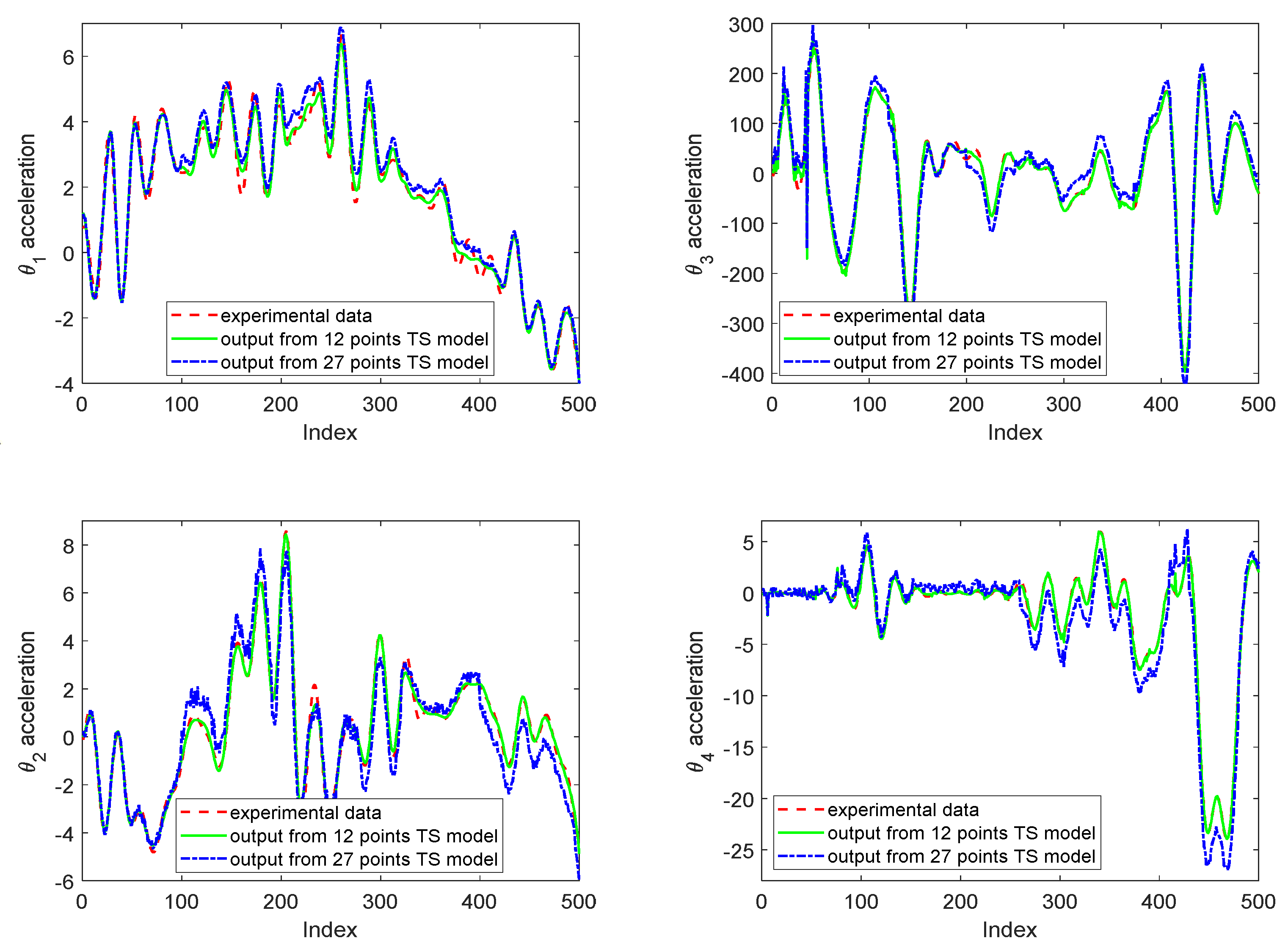
In Figure 5, it can be seen that the outputs predicted by the T-S fuzzy models are very close to the testing experimental data. The NDEIs of the neuro-fuzzy model and the two T-S fuzzy models, which are used as the criteria of global approximation, are listed in

Table 3. NDEIs of the neuro-fuzzy model and T-S fuzzy models.

	Neuro-Fuzzy Model	T-S Fuzzy Model with Uniformly Distributed 27 Points	T-S Fuzzy Model with Optimized 12 Points
NDEI	0.0267	0.0697	0.0477

. It can be seen that the T-S fuzzy models derived from the neuro-fuzzy model can provide an accurate approximation of the original nonlinear system. The 12 points T-S fuzzy model with optimized operating points gives an even better approximation than the 27 points one with uniformly distributed operating points.

To test the controller performance, the reference commands to be tracked are given by

$$r_{{\theta }_1}=r_{{\theta }_2}=\{\begin{array}{cc}0.4t^2& t\le 0.4\\ 0.064+0.32\left(t-0.4\right)& 0.4<t\le 1.875\\ 0.6-0.4{\left(t-2.275\right)}^2& 1.875<t\le 2.275\\ 0.6& t>2.275\end{array}.$$

(26)

Because the gear ratio is 5, the command inputs for θ₃ and θ₄ are given by

$$\begin{array}{cc}{r}_{{\theta }_3}=5r_{{\theta }_1}& r_{{\theta }_4}=5r_{{\theta }_2}\end{array}.$$

(27)

The command inputs for the angular velocities are

$$\begin{array}{l}{r}_{{\dot{\theta }}_1}=r_{{\dot{\theta }}_2}=\{\begin{array}{cc}0.8t& t\le 0.4\\ 0.32& 0.4<t\le 1.875\\ -0.8\left(t-2.275\right)& 1.875<t\le 2.275\\ 0& t>2.275\end{array}\\ \begin{array}{cc}{r}_{{\dot{\theta }}_3}=5r_{{\dot{\theta }}_1}& r_{{\dot{\theta }}_4}=5r_{{\dot{\theta }}_2}\end{array}\end{array}$$

(28)

The performance index is defined as:

$$J={\displaystyle {\int }_0^4\left\{\begin{array}{l}\mathrm{10,000}\left[{\left({\theta }_1-r_{{\theta }_1}\right)}^2+{\left({\theta }_2-r_{{\theta }_2}\right)}^2\right]+\left[{\left({\theta }_3-r_{{\theta }_3}\right)}^2+{\left({\theta }_4-r_{{\theta }_4}\right)}^2\right]\\ +1000\left[{\left({\dot{\theta }}_1-r_{{\dot{\theta }}_1}\right)}^2+{\left({\dot{\theta }}_2-r_{{\dot{\theta }}_2}\right)}^2\right]+\left[{\left({\dot{\theta }}_3-r_{{\dot{\theta }}_3}\right)}^2+{\left({\dot{\theta }}_4-r_{{\dot{\theta }}_4}\right)}^2\right]+0.1T_1^2+0.1T_2^2\end{array}\right\}dt}$$

(29)

The fuzzy optimal control systems derived from the T-S fuzzy models with 27 and 12 points were simulated using the mathematical model in MATLAB with initial condition x = 0. To obtain an assessment of the proposed control algorithm, it is necessary to compare this paradigm to alternative control techniques. Therefore, a PID controller was also designed:

$$\left[\begin{array}{c}{T}_1\\ T_2\end{array}\right]=\left[\begin{array}{c}0.4e_1+0.1{\dot{e}}_1+0.1{\displaystyle \int e_{1}dt}\\ 0.4e_2+0.1{\dot{e}}_2+{\displaystyle \int e_{2}dt}\end{array}\right],$$

(30)

where e₁ and e₂ are tracking error of θ₁ and θ₂. The PID gains were based on [32], in which a PID controller was designed for this robot manipulator. Figure 6 shows the simulated responses of the flexible robot system with the fuzzy controllers and PID controller, while the mean square errors (MSEs) of command tracking are compared in

Table 4. MSEs of command tracking with the designed controllers.

	T-S Fuzzy Model with 27 Points	T-S Fuzzy Model with 12 Points	PID
θ1	2.95 × 10−4	2.98 × 10−4	1.20 × 10−3
θ2	7.31 × 10−4	8.06 × 10−4	1.22 × 10−3
θ3	0.0169	0.0170	0.0744
θ4	0.0084	0.0097	0.0268

. The performances of the fuzzy controllers are evidently better than that of the PID controller. The PID responses exhibit larger overshoot and longer settling time, which leads to larger MSE. The results of the 12 points T-S fuzzy model are almost the same as the results of the 27 points one, as the non-significant difference of modeling errors may only yield trivial effect on the control system. Since the number of linearization is reduced, the 12 points T-S fuzzy model is more computationally efficient.

The fuzzy optimal controllers were then implemented on the robot. The experimental results are shown in Figure 7. The achieved tracking performances are good and close to the simulation results, except for some lags and oscillations along the trajectories. These oscillations are caused by the flexible joints of the robot, which are very difficult to completely eliminate.

6. Conclusions

An explicit procedure of establishing the T-S fuzzy models of unknown nonlinear systems from experimental data is presented: (1) the local constituent models are obtained by direct linearization of neuro-fuzzy models trained from data so that they are close approximations to the local linearization of the original nonlinear systems; (2) The operating points for linearization are optimized using the evolutionary strategy to achieve good global approximation with a reduced number of linearization. The controller design based on T-S fuzzy model has also been discussed. The derived fuzzy optimal controller was applied to a nonlinear flexible-joint robot system and compared with the alternative control technique, which demonstrated the effectiveness of the proposed method for controlling nonlinear dynamic systems whose analytical models are not available. Compared with the existing T-S model methods, the proposed method could more effectively address the tradeoff between local and global approximation for complex systems. Moreover, since the computational methods of the proposed method are based on a set of well-developed tools (e.g., FBFN training, ES optimization), it can be readily used for data-driven system identification and controller design in realistic applications. The future work might include studying the effect of uncertainty in data and the modeling errors of the neuro-fuzzy and T-S fuzzy models, such that the robustness of the T-S fuzzy control scheme can be more explicitly addressed.