Coarse Return Prediction in a Cement Industry’s Closed Grinding Circuit System through a Fully Connected Deep Neural Network (FCDNN) Model

Abstract

Milling operations in various production processes are among the most important factors in determining the quality, stability, and consumption of energy. Optimizing and stabilizing the milling process is a non-linear multivariable control problem. In specific processes that deal with natural materials (e.g., cement, pulp and paper, beverage brewery and water/wastewater treatment industries). A novel data-driven approach utilizing real-time monitoring control technology is proposed for the purpose of optimizing the grinding of cement processing. A combined event modeling for feature extraction and the fully connected deep neural network model to predict the coarseness of cement particles is proposed. The resulting prediction allows a look ahead control strategy and corrective actions. The proposed solution has been deployed in a number of cement plants around the world. The resultant control strategy has enabled the operators to take corrective actions before the coarse return increases, both in autonomous and manual mode. The impact of the solution has improved efficiency resource use by 10% of resources, the plant stability, and the overall energy efficiency of the plant.

1. Introduction

The cement manufacturing process is comprised of a number of sub-operations such as quarrying, crushing, raw milling, burning, cooling, and cement grinding. The control of cement grinding is an essential part of the process of cement production. It has remained a challenging problem for years because of the existing model uncertainties, nonlinearities, variation in the feedstock, and multi-factor interdependencies. Modeling, optimization, and control of integrated grinding circuits are some of the major challenges in the efficiency and productivity of cement production systems. Minimizing energy consumption while simultaneously improving product quality and process efficiency would be a major contribution to the cement industry, and reduce global energy consumption and greenhouse gas emissions [1,2,3,4,5]. However, the large non-linear nature of the process poses major challenges for creating feasible control tactics to maintain process stability and increase efficiency and productivity. Therefore, in our experience of more than 20 years in dealing with cement production, predicting the events that affect the production process is highly desirable, and with the recent technological advancements in real-time data acquisition and analytics becomes achievable in practice. This predictive capability to look ahead to the quality-related variables in the milling plant will allow the use of corrective control policies in order to improve the stability of the system. In our view, such capabilities can be deployed in any industrial setting that has a similar closed-loop controlled milling process regardless of the raw material (e.g., pulp and paper, beverage brewery and water/wastewater treatment industries).

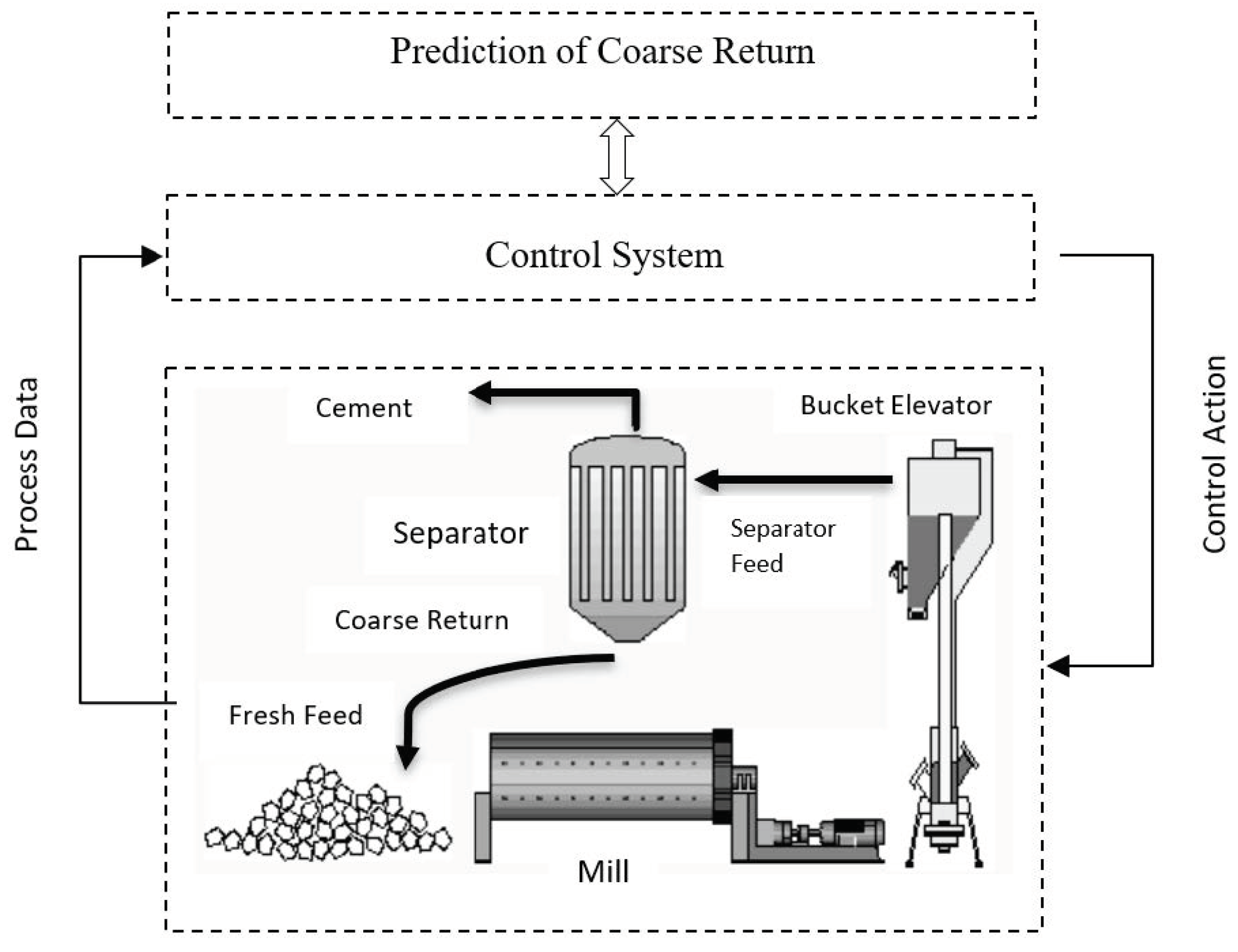
Figure 1 shows a schematic of a closed-loop cement grinding process control system [6]. Inside the rotating ball mill, the feed flow supplies raw material (natural stones of various sizes and humidity) to be ground by steel balls. A bucket elevator is used to transport the mill product into the separator where depending on adjustable airflow rate and speed, it is divided into a flow of rejected oversized particles (named coarse return), which are returned to the mill inlet to be ground again (grinding mostly is performed in closed circuit) and a flow of fine particles, which forms the final product.

In the cement grinding process, coarse return is one of the main parameters of the process, representing the product quality output. It has a major role in setting the optimization and control objective function of the closed-loop process. Measurement of coarse returns allows for better control of process efficiency as variations in the performance of the grinding circuit occur over time. Understanding the basic and interaction effects of the mill and separator variables on coarse return is an essential factor of the process improvement and is the motivation of this study. In particular, if the coarse returns flow rate increases, then the production flow needs to be reduced so as to not aggravate the increased quality problem. Predicting coarse return helps with stabilizing the process by controlling the controllable system’s parameters such as fresh feed and/or separator’s speed. Nevertheless, grinding is an unstable and complex process whose variables have coupling, time-varying delay, and non-linear characteristics caused by natural variation, mill load, and fluctuation of the raw material hardness and grindability. It leads to obstruction of the mill and interruption of the grinding process. The phenomenon is known as ‘plugging’ which increases the complexity of process control and optimization by conventional multivariable data analytics and machine learning methods.

This paper proposes a fully connected deep neural network (FCDNN) model to predict the upcoming coarse return in the cement grinding process up to 15 [min] ahead. The choice of FCDNN is for the reason that deep learning has a stronger model expression ability to produce a good fit for highly non-linear system behavior and the associated data of the complex interactions of the grinding system and, consequently, better prediction accuracy. Our further experience in practice validates and verifies its ability to capture the complexity of the grinding process accurately in the plant that the model was evaluated. This will be proved by the comparison of the results with other NN methods in the industry. In the following, we will review the existing literature on the cement grinding process prediction and optimization.

Related Works

Modeling and simulation of the cement grinding process are efficient tools for predicting and optimizing the process [7]. Modeling grinding circuits should consider several grinding operational variables such as the mill and separator details to name a few. In recent years, many strong grinding process simulation models have been developed to date. These models of industrial grinding circuits can be considered robust and highly accurate [8,9]. The majority of the proposed models reported in the literature are a combination of physical laws of conservation of energy state and empirical correlations. Using empirical methods, an inferential model was necessary for many models as the real physics behind the phenomena is not very clear. This brings the necessity of constructing end-to-end model mapping of the inputs and the outputs of a grinding plant, possibly needing a grey box or black box method approach to solve the problem. One efficient solution to these problems is building data-driven dynamic models for integrated grinding circuits [2,7]. These models are trained only on data collected from inlet and outlet streams of the grinding circuit and result in multiple-input-multiple-output (MIMO) system identification models.

For advanced modeling of complex and non-linear dynamics process operations where an accurate mathematical model cannot be established, intelligence-based advanced methods have drawn the increasing attention of researchers [10]. Availability of a large amount of acquired data as an outcome of the deployment of advanced instruments, sensors, and novel networking technologies, which was not usually possible in the past, also justify this attention. Therefore, studying intelligence-based advanced methods by combining a large amount of production process data along with empirical knowledge of operators is an effective way to solve the advanced control problems in complex industrial applications where accurate mathematical models are difficult to establish [11].

The main characteristic of artificial intelligence (AI) technologies and machine learning (ML) techniques is their ability to emulate human reasoning through data and knowledge while avoiding human subjectivity and arbitrariness. Thus, with the growth in the development of AI and ML techniques in the recent past, the interest has shifted towards studying these techniques, and they have been widely used to deal with modeling and control problems of complicated industrial processes. Deep neural networks (DNNs) are examples of data-driven ML methods that have the characteristics of quick response and complex non-linear approximation to process with characteristics of nonlinearity, time-varying delay, and coupling. Therefore, DNNs are widely applied for non-linear problems in regressive prediction and show good performance in solving non-linear problems [3,12,13,14]. For example, the recurrent neural networks (RNNs) (which is a type of DNN) methodologies are used to compete with prominent system identification tools, such as wavelet networks to model time series data [15,16]. Long short-term memory (LSTM) networks are RNN-based methods capable of extracting features shared over an extended range of time and can be used with ML methods such as the regression method [17,18]. However, although RNNs including LSTMs were used for modeling sequential data for a few decades, their success in system identification was limited due to their inability to capture significantly long-time delays in-process data. Moreover, these are heuristic methods, and their performance is highly dependent upon the experience of users and they are challenging to implement [19].

Another NN method widely used in system identifications of complex non-linear processes is the modeling method based on the radial basis function (RBF) NN due to its simple structure, straightforward training, and fast learning convergence, and ability to approximate arbitrary non-linear function. However, its time consuming and slow application is its main disadvantage in real-time applications [20].

In [21,22], two research works have been conducted on the modeling of the fineness of particles in the milling circuit to control a cement mill better. These research works have tried to explore the relationship between the particle size of cement produced (a quality performance indicator) and various mill parameters and consequently provide a model for predicting Blaine (fineness of particles). Different data-driven non-linear models including LSTM and multilayer perceptron (MLP) results on a cement mill dataset have been compared and concluded that predictive models’ accuracy highly depended on the cement mill dynamics.

The contribution of this research lies first in the prediction of coarse return for process control in cement plants which is not yet delivered in the literature. This study aims to leverage recent advances in deep learning techniques to propose an FCDNN model to predict the upcoming coarse return in a cement grinding process. In the next section, we describe a real-world cement industry’s closed grinding circuit system use case and the data collection campaign alongside the proposed FCDNN model. This will be followed by a review of the deployed model’s behavior in the dynamics of the complex operations and prediction results. Section 4 discusses the results and comparison and evaluation with two other methods. Finally, this study is concluded by a conclusion and future research direction.

2. Materials and Methods

In this section, the used materials, including the collected data, preparation, and use case, will be explained. This will be followed by the proposed FCDNN techniques structure and implementation.

2.1. Data Collection and Preparation (Sampling Campaigns)

A one-month data collection campaign was run in a real grinding process plant. A total number of 45 process variables of the mill and separator were acquired through DataBridge technology. DataBridge is a propriety Control Area Network (CAN) application to connect the process control data acquisition and monitoring devices to the process optimizer. [23]. One of the main challenges during the sampling of a continuous process is choosing the right sampling rates. The choice of a proper sample frequency may avoid information annihilation (i.e., low frequency) or pre-process for data segmentation and aggregation due to the collecting of similar data (i.e., high frequency). In [24] (p. 57), one of the methods proposed for the sampling of continuous signals in system identification was:

$$T \approx {\mathsf{\tau }}_{\min }/3$$

(1)

where τ_min is the shortest process time constant, and T is sampling time.

In our experimentation, the study of process signals showed the shortest process time constant was about three minutes. Then, according to Equation (1), the data sampling rate of the system was set at a sample per minute. That meant a collection of about 43,000 samples in a month timeframe.

2.1.1. Filtering the Outliers

Any measurement out of the normal operation range had been filtered out as the outliers. These ranges were acquired from operators.

2.1.2. Filtering out the Irrelevant Inputs

Event-Modeling is a technique for real-time input variable selection in large complex systems [25]. This method is able to group and rank relevant input variables in order of their importance and impact on the model output variable(s). It does not require prior knowledge of the analytical or statistical relationship that may well exist between system input and output variables. This method supports the time-critical dimensionality reduction problem with limited computational resources, which made it suitable for feature extraction and dimensionality reduction in this experiment.

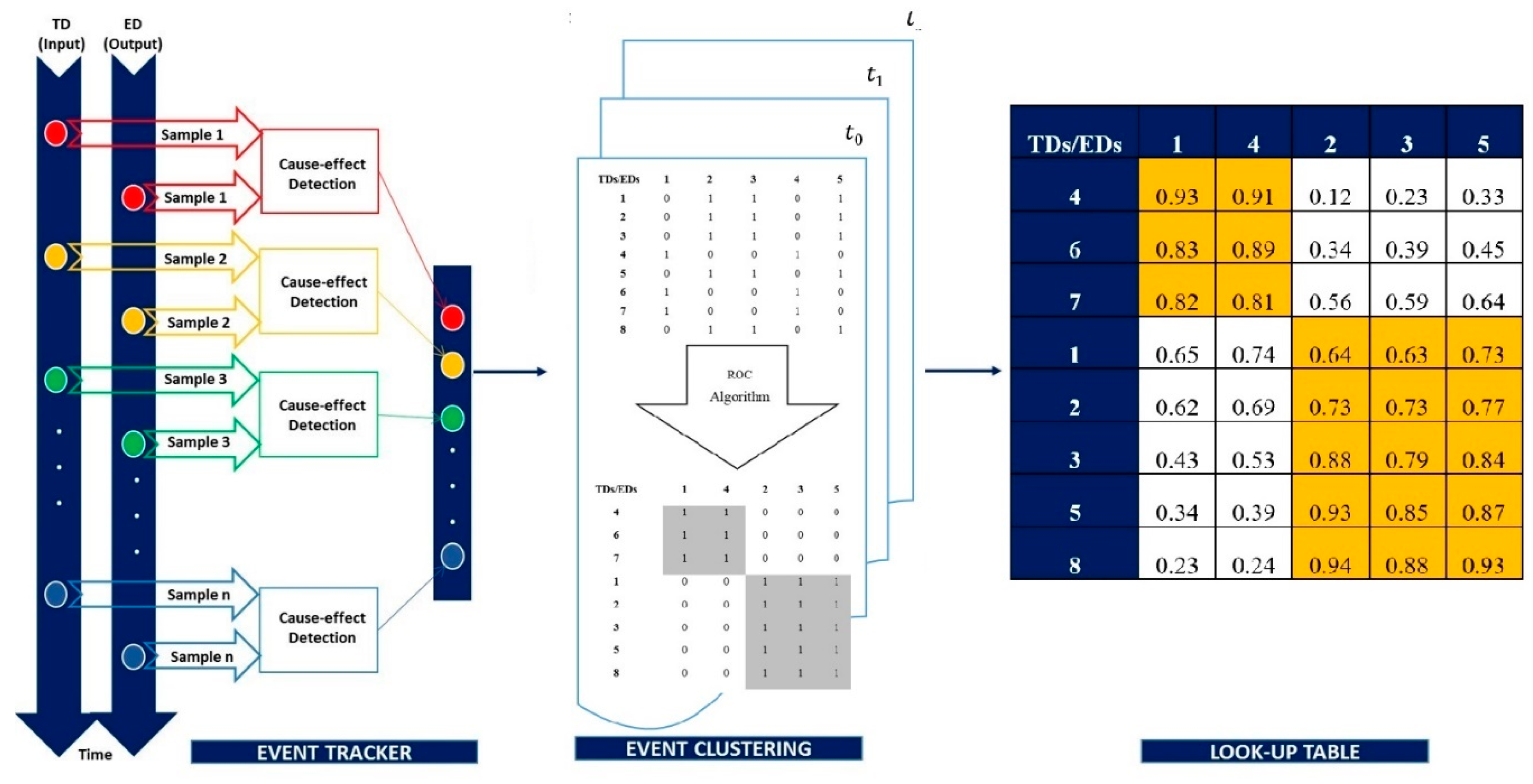
The event-Modeler algorithm was based on evaluating the relationship between the actual events (model’s output variables) to the triggered events’ cause (model’s input variables). The input/output pairs were used to generate the event-driven incidence matrices (EDIM) element. The application of the ranking ordering clustering (ROC) method resulted in clusters of the most relevant group of input event data (sensors and actuators) against output event data (plant performance indicators). Event tracking, EDIM, and final clustering matrix are presented in Figure 2. As shown in this example, the final clustering table is the normalization of a single event clustering matrix over the sampling time frame.

Consequently, the algorithm clustered the input/output variables in two groups of highly coupled clusters. i.e., input variables (TDs) 4, 6, and 7 had high impacts on output variables (EDs) 1 and 4 and the same interpretation for the other cluster. A detailed explanation of the event-modeling algorithm and the basic concept is discussed in [25,26].

In this experiment, 33 collected process and environmental variables were considered as the event-modeler input variables and coarse return as the output variable. The six highest-ranked (coupled) input variables over output (coarse return) were considered as the most important input variables following the industry expert’s approval. The event-modeler correlation results between the input parameters and output (coarse return) are shown in

Table A1. Event-Modeler output between the mill and separator parameters and coarse return.

Input Variables	Event-Modeler’s Output	Subjective Importance Level
SEA	92%	High
SES	92%	High
FEF	87%	High
MIF	86%	High
MOF	82%	High
BEA	75%	High
Separator Temperature	68%	Medium
Mill Power	64%	Medium
Mill Power Transducer	62%	Medium
Fresh Feed Mill excs Setpoint	60%	Medium
Fresh Feed Scada Setpoint	60%	Medium
Separator Mill excs Setpoint	59%	Medium
Separator Scada Setpoint	58%	Medium
SURECAST Cement	57%	Medium
Recycle Elevator Current	54%	Medium
Cement Surface Area	52%	Medium
Cement Residue	51%	Medium
High Counter	49%	Low
Low Counter	49%	Low
High-Quality Counter	48%	Low
Blaine minus one	48%	Low
Previous Blaine	46%	Low
Test Quality Counter	45%	Low
Higher Blaine Counter	44%	Low
Lower Blaine Counter	44%	Low
Inlet objective	43%	Low
Opc Cement	40%	Low
Ubc Cement	40%	Low
Out of Spec	36%	Low
Current Max feed	33%	Low
Total Charge	32%	Low

in Appendix A. These six inputs were the following; the mill’s four parameters of:

• Fresh feed (FRF): Measured the amount of material that was being fed to the mill [ton/h].
• Mill inlet fill (MIF): Measured the filling level on the first chamber of the mill [%].
• Mill outlet fill outlet (MOF): Measured the filling level on the second chamber of the mill [%]
• Bucket elevator amperage (BEA): Transferred the mill outputs to the separator in amperes [A].

Plus, two separator parameters of:

• Separator Amperage (SEA): This amperage was used by the separator; it was dependent on the amount of incoming load [A].
• Separator Speed (SES): Defined the separator velocity (related with final cement quality, manually set by operators).

Altogether, these six parameters were the model inputs. In addition, the model output was:

• Coarse return (COR) [ton/h].

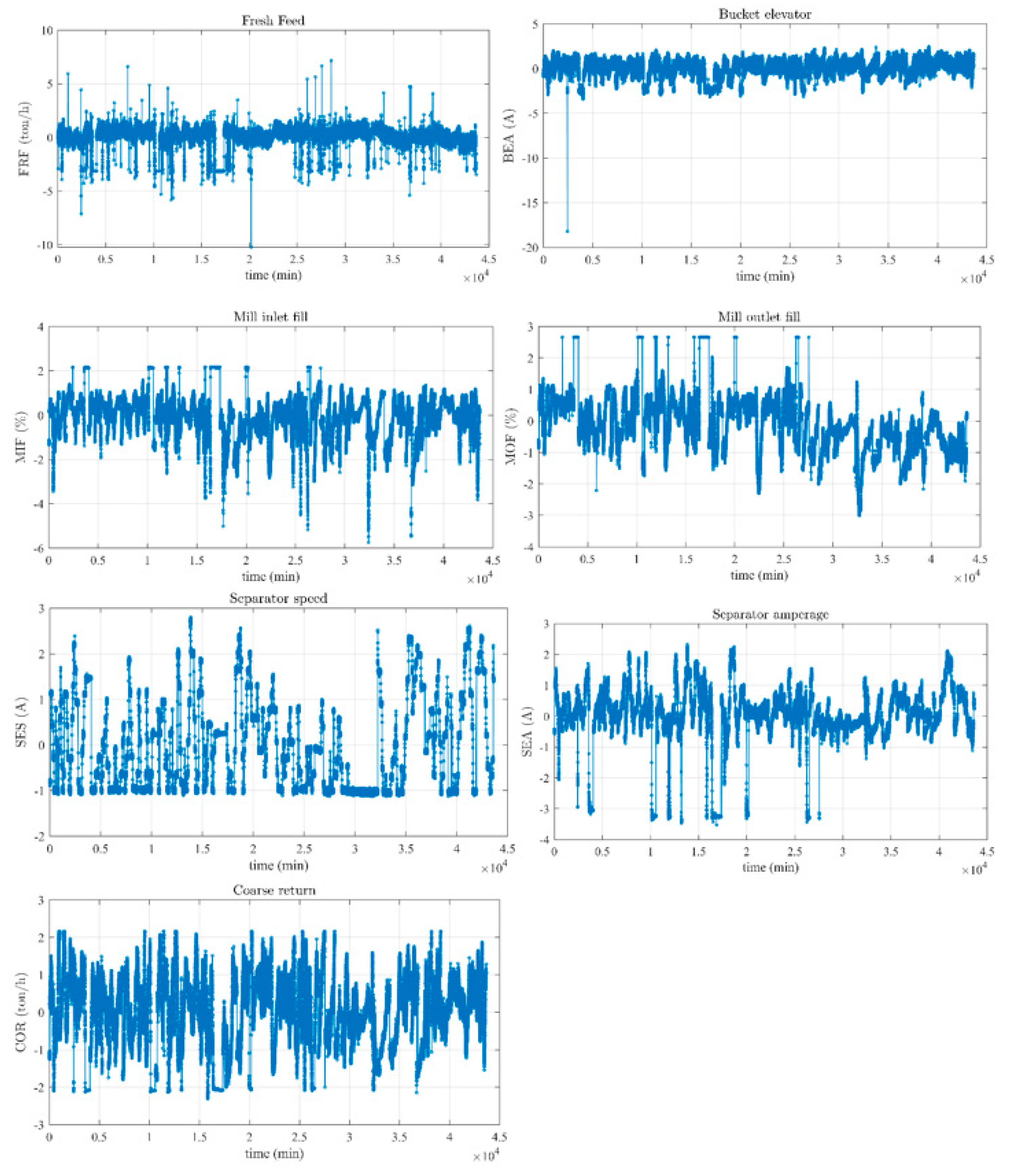
The plots of each variable are shown in Figure 3. The plots are normalized for confidential purposes.

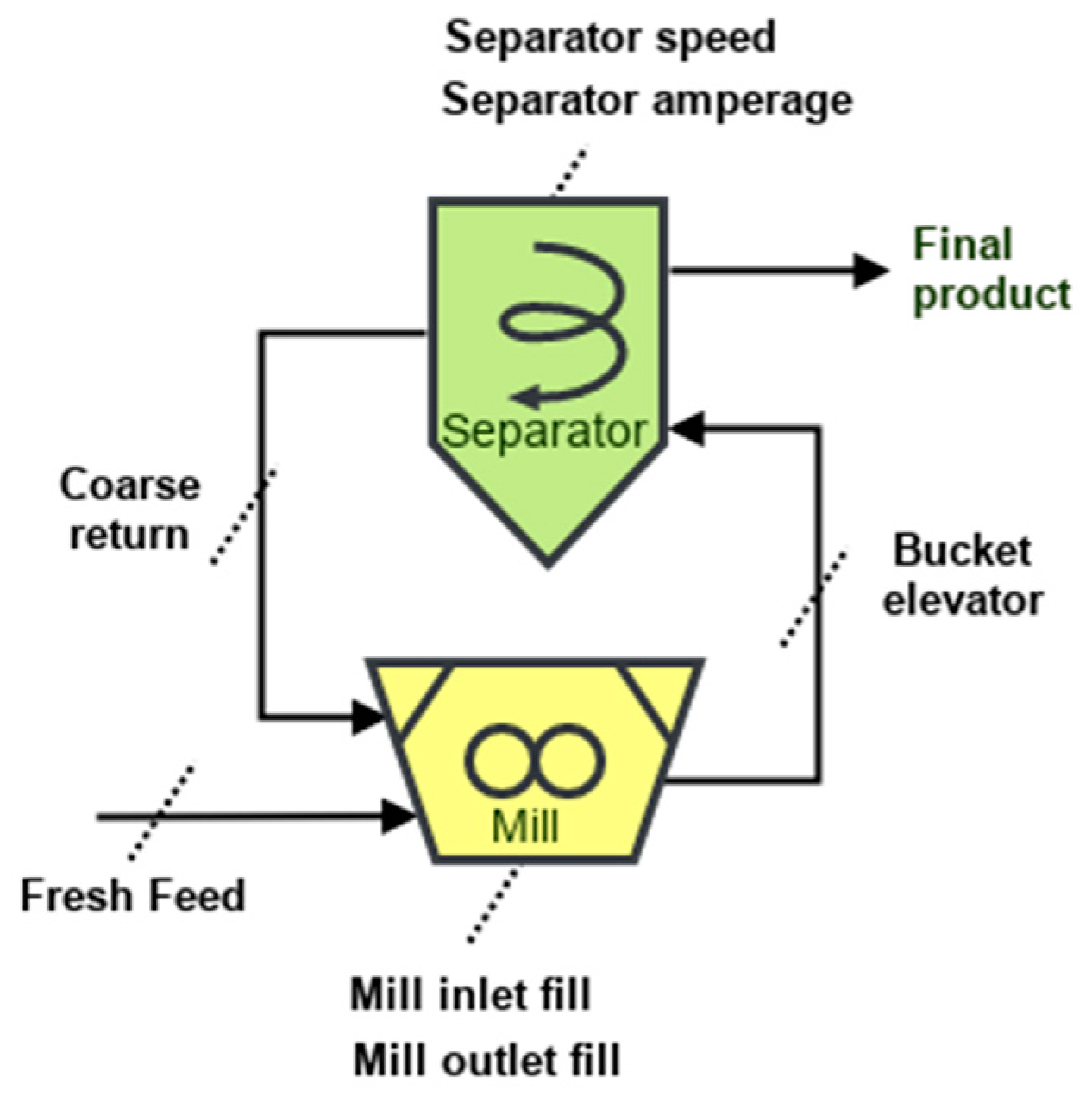
A schematic of the shortlisted mill and separator parameters, including the coarse return feedback loop as presented in Figure 4.

2.1.3. Delays Estimation

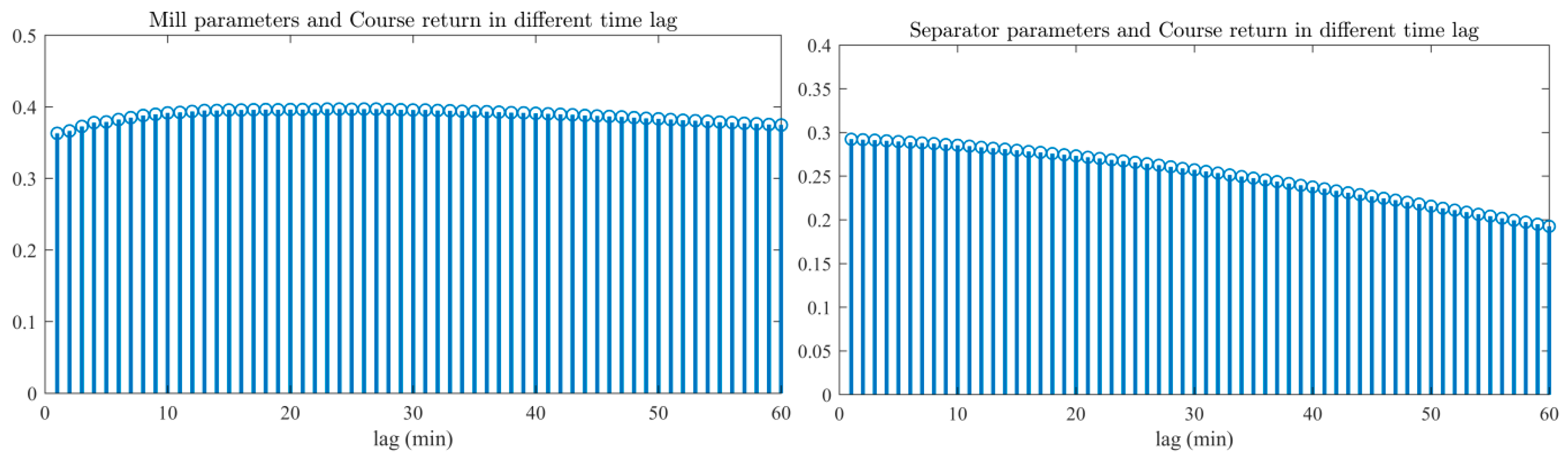
Delays interactions are a ubiquitous feature of many dynamical systems, including the cement industry. Therefore, time delays played a fundamental role in our experiment. Noteworthy, the time delay was non-linear and caused complex dynamic behavior, which could not be explained by just looking at the constituents of a system. These delays were between the mill and separator parameters and the coarse return. To simplify the non-linear delays, a cross-correlation analysis time delays estimation [27] was conducted between the mill and separator parameters and coarse return. This technique was used to determine the temporal relationship between process variables. By finding the highest absolutes cross-correlation for various lag times, an average delay time between the two variables could be determined. For example, the time lag between mill parameters (i.e., FRF, MIF, MOF, and BEA), and coarse return varied between 1 to 60 min, but in minute 23, the cross-correlation was in the maximum. This time lag for separator parameters (i.e., SEA and SES) and coarse return is almost null. Figure 5 shows the applied cross-correlation technique results between the mill and separator parameters and coarse return variable with different time lags.

2.2. Fully Connected Deep Neural Networks

NN algorithms are extensively used by machine learning and data scientists for solving different kinds of data regression and classification problems. Artificial NN (ANN) has proven in many applications to be a robust data modeling tool capable of capturing and representing complex input/output relationships. They are a human brain-inspired programming paradigm that allows a computer to learn from observational data similar to the brain.

Fully-connected deep neural networks (FCDNNs) is a member of a general class of feedforward neural networks. An FCDNN takes in vector data as an input and outputs a vector. An FCDNN is made up of several fully connected layers and each fully connected layer consists of multiple nodes. Data enters the FCDNN via the input layer nodes. Each node (excluding input layer nodes) is connected to all nodes in the earlier layer. The values at each node are the weighted sum of node values from the previous layer. The weights are the trainable parameters in FCDNN. The outputs of the hidden layer nodes typically go through a non-linear activation function, e.g., exponential linear units, while the output layer tends to be linear. The value at each output layer node typically represents a predicted quantity. Therefore, FCDNNs allow the prediction of multiple quantities simultaneously.

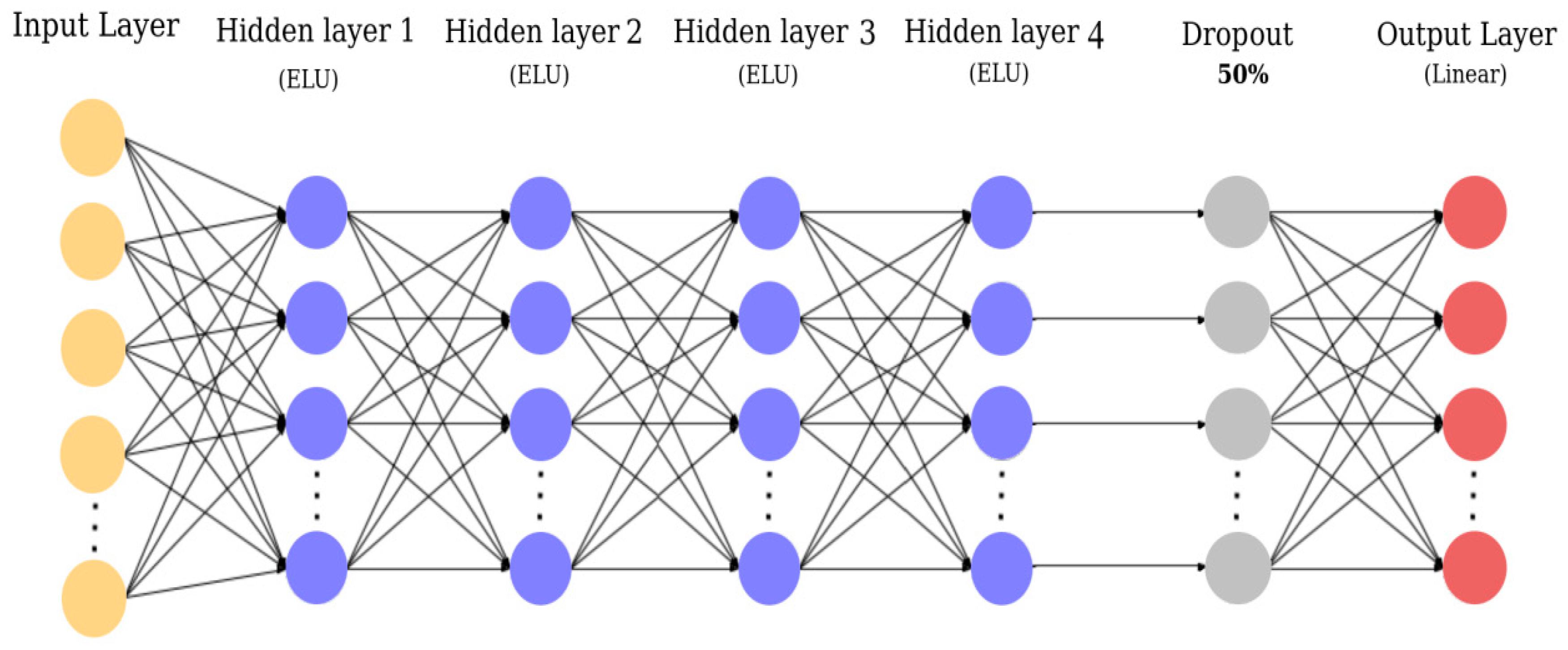
Fully connected networks are a subcategory of deep neural networks. These networks are ‘Structure Agnostic’ and are fully connected networks [28]. The structure of the proposed FCDNN developed for this study is represented as follows in Figure 6.

2.2.1. FCDNN Structure

The FCDNN used in this study had a six-layer network structure, consisting of an input layer, four hidden layers, and an output layer, each composed of a plurality of neurons that could be calculated in parallel. The connection between the hidden layers and between the first hidden layer and the input layer was connected by an activation function. The details of the structure of the proposed FCDNN are as following:

(A)

Fully-connected layer (or dense layer)

The fully connected layers were able to learn non-linear combinations of input features considerably efficiently. Neurons in a fully connected layer have full connections to all activations in the previous layer. Their activations can hence be computed with a matrix multiplication followed by a bias offset [29]:

$$H\left(x\right)=Wx+b,$$

(2)

where $W\in R^{\left(K,n\right)}$ is the weight matrix and $b\in R^K$ is the bias offset.

(B)

ELU activation layer

Exponential Linear Unit (ELU) is a function that tends to converge cost faster and generate more accurate results [30]:

$$\mathrm{ELU}\left(\mathrm{x}\right) = \left\{\begin{array}{c}\alpha \left(e^x-1\right) if x\le 0\\ x if x>0\end{array}\right\}$$

(3)

ELU uses the activation function in order to achieve mean zero, as the learning can be made faster. For the ELU activation function, an α value is picked; a common value is between 0.1 and 0.3. Hence it is a good option against activation functions like ReLU (Rectified Linear Unit) since it decreases the bias shift by pushing the mean activation towards zero. Unlike ReLU, ELU can produce negative outputs.

(C)

Dropout layer

Dropout is a sort of regularisation that randomly drops some proportion of the nodes that feed into a fully connected layer. Dropping a node means that its contribution to the corresponding activation function is set to zero, and therefore it prevents the network from memorizing the training data (overfitting). With dropout, training loss will no longer tend rapidly toward zero, even for extensive deep networks.

(D)

Linear activation layer

A linear activation function takes the form [28]:

$$A=cx,$$

(4)

where c is a constant number and activation is proportional to the input. This way, it provides a range of activations, so it is not binary activation.

2.2.2. Loss and Optimization Functions

In most learning networks, the error is determined as the difference between the actual output and the predicted output [28]:

$$\left(w\right)=p-\widehat{p},$$

(5)

where $J$ is a function of internal parameters of model, weights, and bias. The function that is used to compute this error is known as the loss function.

Different loss functions will provide different errors for the same prediction, and therefore have a considerable effect on the performance of the model. One of the most widely used loss functions is the mean absolute error (MAE) that was used in this research, which calculates the absolute of the difference between the actual value and predicted value. Various loss functions are used to deal with different types of tasks, i.e., regression and classification.

For accurate predictions, minimization of the calculated error functions is needed. In a NN model, the weights and biases are modified using a function called the optimization function. Some important first-order optimization functions are Adaptive Moment Estimation (Adam), Stochastic Gradient Descent, and Adagrad [30]. It also calculates a different learning rate. Adam works well in practice, is faster, and outperforms other techniques, and was used in this paper with a learning rate set to 0.01.

2.3. The Proposed FCDNN Implementation

For this experiment, the proposed architecture was the application of an FCDNN and several hyperparameters that had to be determined, including the number of fully connected layers, the number of nodes in the fully connected layers, dropout, etc. The presented network settings in

Table 1. FCDNN layer types, output shapes, and parameters number.

Layer (Type)	Output Shape	Parameters Number
Hidden layer 1 (Dense)	(None, 30)	870
ELU 1	(None, 30)	0
Hidden layer 2 (Dense)	(None, 90)	2790
ELU 2	(None, 90)	0
Hidden layer 3 (Dense)	(None, 80)	7280
ELU 3	(None, 80)	0
Hidden layer 4 (Dense)	(None, 70)	5670
ELU 4	(None, 70)	0
Dropout 1	(None, 70)	0
Output (Dense)	(None, 4)	284

were set after several comparative experiments, which showed that this combination produced the best performance for the network. Hidden layers (dense layers) 1 to 4 were features extraction, the ELU layer was added at the end of every dense layer for accelerating the training speed, and the dropout layer was added after the third dense layer to avoid the extraction of redundant features and prevent the over-fitting problem which regularly occurs in deep neural networks [31].

2.3.1. Model Structure.

There was about 43,000 min of data. Each data sample consisted of separator actual speed, fresh feed, mill fill inlet, mill fill outlet, bucket elevator amperage, separator amperage, and coarse return variables. The input for each FCDNN was a vector ($28\times 1$) of current states (system parameters and coarse return) and three previous states.

The output vector dimension was $\left(4\times 1\right)$ which denoted the predicted coarse return of the next 1, 5, 10, and 15 min, respectively.

Training a NN is the process of finding the values for the weights and biases. The training of a NN model is most challenging because it requires solving two hard problems at once: learning and generalizing. Learning the training dataset is to minimize the loss function while generalizing the model performance is to make predictions on test examples (validation dataset). If a model learns too well, it will generalize poorly (overfitting), and if a model generalizes well, it may result in underfitting. One of the objectives in training a NN is to obtain a good balance between these two problems.

In this experiment, the existing approximate 43,000 sample data with a sampling rate of 1 sample/minute were randomly split into a training dataset (typically 90 percent of the data), a validation dataset (10 percent of data). After training was completed (5000 epochs), the trained model’s weights and the biases were deployed and tested on the test dataset. One of the significant difficulties when working with NNs is overfitting. Model overfitting often occurs when the training algorithm runs too long. The validation helps identify when model overfitting starts to occur by keeping the model parameters.

2.3.2. Training Dataset

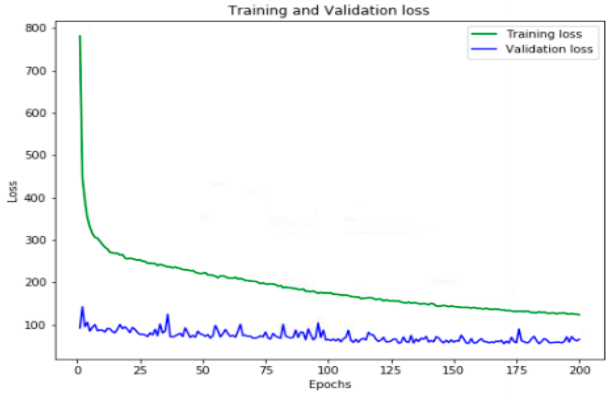
The validation error was lowest during the training. Figure 7 shows the training and validation data loss curve for predicting network parameters after 200 epochs. Our results showed the proposed model could perfectly keep the balance between learning and generalizing.

3. Results

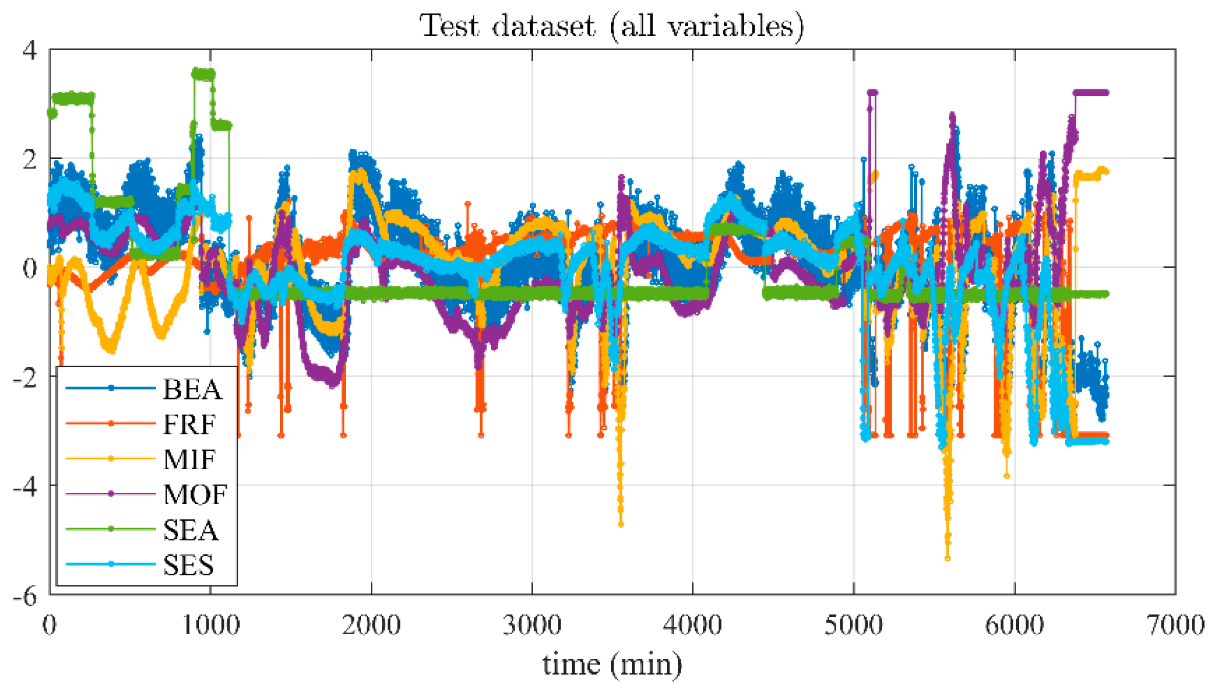
A test dataset was collected every minute for 108 h (i.e., 6500 samples). The collected data had been pre-processed and the estimated time-delay (explained in Section 2.1) had been conducted and then applied to the trained model. Figure 8 shows the test dataset of input parameters. The objectives were the prediction of upcoming coarse return for 1, 5, 10, and 15 min later.

Table 2. Mean absolute error (MAE) and average variation between the actual and predicted coarse return on the test dataset.

Method/Prediction Time	1 min	5 min	10 min	15 min
MAE	4.78	8.82	13.68	18.06
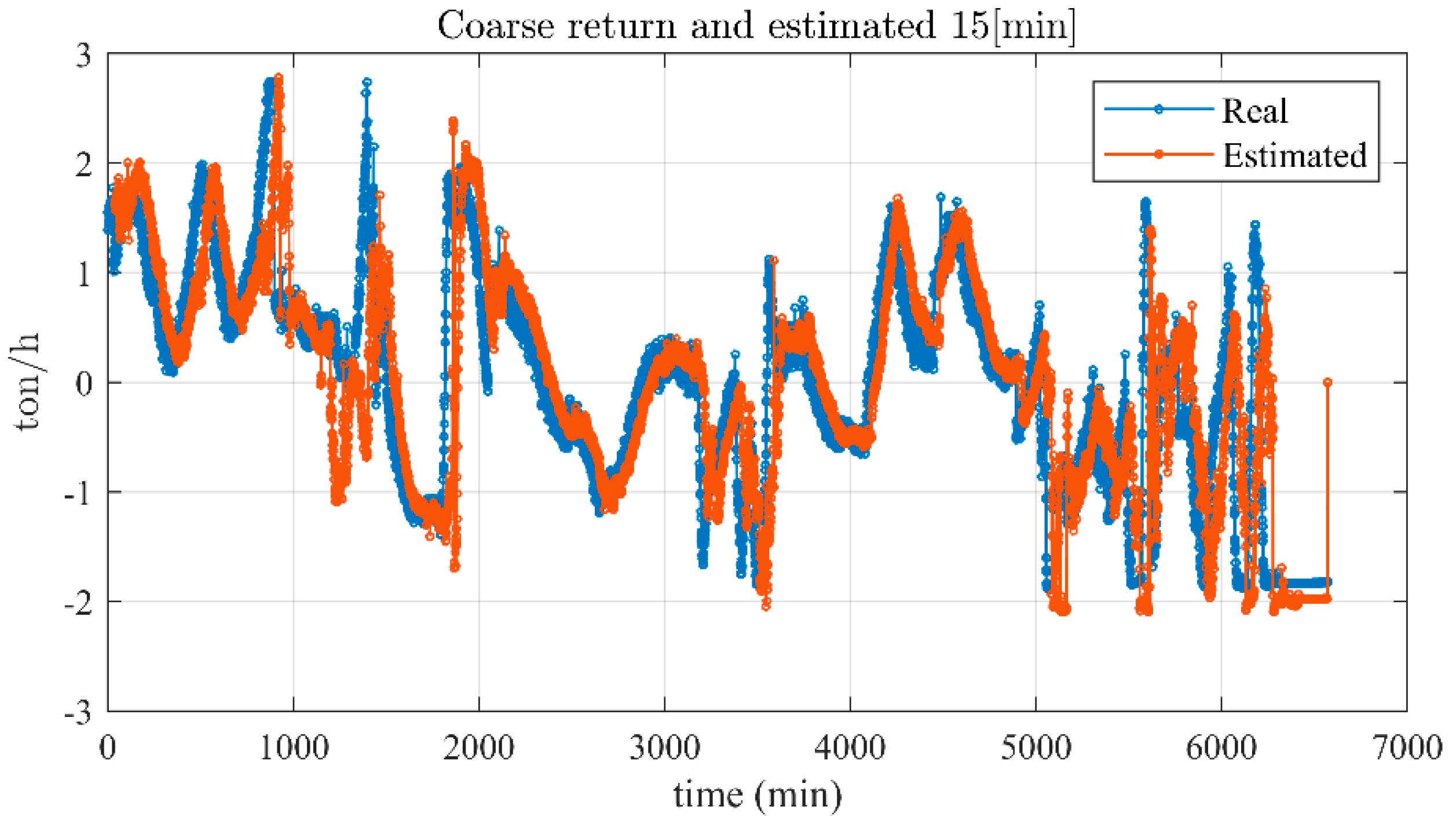
Average deviation %	5.2	9.74	15	19.9

presents the MAE and average deviation (MAE/average coarse return) between the actual coarse return and its future predictions. These two comparison methods were chosen due to their extensive applications in the comparison domain. Based on the presented results, the coarse return for the next minute was predicted with 95% overall accuracy, and then for the prediction for every single minute ahead, the accuracy dropped by 1%, for example, for a quarter-hour ahead forecast, its accuracy was about 80%.

Noteworthy, the cement grinding process variables, as seen in Figure 3, had a complex, non-linear and unstable process causing plugging phenomena. The extracted features (6 inputs and single output) of the process control using the proposed techniques and the trained model was successfully validated and verified in practice and by the cement production engineers. The accuracy of the proposed method was also compared with the single-layer NN and LSTM, to demonstrate its superior performance against two other rival and relevant approaches.

Figure 9 presents the actual coarse return and those predicted for the next 15 min in a single graph.

4. Discussion

Due to the feedback loop in the process, the prediction of the future amount of coarse return has more uncertainty because prediction errors would be accumulated in the next time frame (minute here) prediction and so on. The certainty of the predictions depends directly on the quantity and quality of the dataset used for the estimation of the models as well as the applied technique. Two other widely used methods in the system identifications of the complex non-linear process have been applied to compare and validate the proposed FCDNN method’s output. The chosen methods were the following two:

4.1. LSTM Method

Due to the LSTM capability of extracting features shared over an extended range of time, LSTMs are known as a well-built technique for challenging sequence prediction problems. A stacked LSTM architecture is represented as an LSTM model involving multiple LSTM layers with the multiple hidden LSTM layers piled one on top of another. Stacking LSTM hidden layers makes the model deeper, more accurately earning the description as a deep learning technique. In this research, we join four of the LSTM layers, each with a dropout layer of value (0.2). In each layer, the number of units is set to 50, showing the dimensionality of the output space. The final layer is the output layer which is a fully connected dense layer.

4.2. A Single Hidden Layer NN Method

A single hidden layer NN method with 100 hidden neurons and ReLU active transfer function was used due to simplicity in its training and deployment.

Both methods applied to the same training dataset include the feedback loop like the proposed FCDNN model. Outputs MAE between the actual and predicted coarse return on the test dataset (presented in Figure 8) for the single-layer NN and LSTM are shown in

Table 3. MAE between the actual and predicted coarse return on the test dataset in long short-term memory (LSTM) and single hidden layer neural network (NN) methods.

Method/Forecasting Ahead	1 min	5 min	10 min	15 min
A single layer NN	8.99	14.07	23.73	23.85
Stacked LSTM	8	11.16	15.88	20.16

. In comparison with FCDNN, they perform worse. The single layer NN has the worst performance in all scenarios, which is comprehensible, due to the more complex and extensive architecture of the proposed approach and the LSTM. The LSTM has a better performance than a single layer NN, but still worse than FCDNN. However, in the training algorithm’s speed and computational complexity, the single-layer NN is on the top and LSTM on the bottom of the table.

5. Conclusions

The operation of a cement grinding circuit is a complex and non-linear process, which makes it difficult to control, optimize and predict the outcome. Coarse return is one of the process parameters which has a major role in the control and optimization of the process, and its prediction is an essential factor of the process improvement. In this paper, an FCDNN architecture for the prediction of the coarse return is proposed. The result of the proposed model shows better accuracy in comparison with two widely used single hidden layer NN and LSTM architectures in the cement grinding process. The LSTM has a better performance than a single layer NN, but still not better than FCDNN. In future works, the LSTM, due to its capacity to deal with long time series prediction, will be further investigated and inserted into our prediction system.

A one-month data collection campaign was run over of a real grinding process plant. The collected dataset contains the essential operating events capturing the variation of the operating conditions of the grinding circuit during the process cycle. It allows the prediction of the coarse return variables with high accuracy. The key variables affecting the coarse return were determined through the event-modeler technique (feature extraction technique), and the prediction model of the system was obtained by using an FCDNN identification.

The proposed method is currently successfully being applied in a number of cement plants, enabling the operators to take corrective actions before the coarse return increase (both in autonomous and manual mode). The impact of the solution has improved efficiency resource use by 10% of resources, the plant stability, and the overall energy efficiency of the plant. The prediction of coarse return in a long horizon is one of the ways to achieve a better performance of cement plants. This is a clear example of the application of artificial intelligence in the cement industry and how it can benefit overall production.

References

- Gao, T.; Shen, L.; Shen, M.; Liu, L.; Chen, F. Analysis of material flow and consumption in cement production process. J. Clean. Prod. 2016, 112, 553–565. [Google Scholar] [CrossRef]
- Altun, O. Simulation aided flow sheet optimization of a cement grinding circuit by considering the quality measurements. Powder Technol. 2016, 301, 1242–1251. [Google Scholar] [CrossRef]
- Miriyala, S.S.; Mitra, K. Deep learning based system identification of industrial integrated grinding circuits. Powder Technol. 2020, 360, 921–936. [Google Scholar] [CrossRef]
- Inapakurthi, R.K.; Pantula, P.D.; Miriyala, S.S.; Mitra, K. Data driven robust optimization of grinding process under uncertainty. Mater. Manuf. Process. 2020, 35, 1870–1876. [Google Scholar] [CrossRef]
- Altun, O. Energy and cement quality optimization of a cement grinding circuit. Adv. Powder Technol. 2018, 29, 1713–1723. [Google Scholar] [CrossRef]
- Kazarinov, L.; Khasanov, D. Decision Making Process for Operational Neurocontrol of Mixture Grinding in Cement Production with Controversial Setting. In Proceedings of the 2019 International Russian Automation Conference (RusAutoCon), Sochi, Russia, 8–14 September 2019; pp. 1–6. [Google Scholar]
- Kwon, J.; Jeong, J.; Cho, H. Simulation and optimization of a two-stage ball mill grinding circuit of molybdenum ore. Adv. Powder Technol. 2016, 27, 1073–1085. [Google Scholar] [CrossRef]
- Zhou, P.; Lu, S.; Yuan, M.; Chai, T. Survey on higher-level advanced control for grinding circuits operation. Powder Technol. 2016, 288, 324–338. [Google Scholar] [CrossRef]
- Minchala, L.I.; Zhang, Y.; Garza-Castanón, L. Predictive control of a closed grinding circuit system in cement industry. IEEE Trans. Ind. Electron. 2018, 65, 4070–4079. [Google Scholar] [CrossRef]
- Lv, L.; Deng, Z.; Liu, T.; Li, Z.; Liu, W. Intelligent technology in grinding process driven by data: A review. J. Manuf. Process. 2020, 58, 1039–1051. [Google Scholar] [CrossRef]
- Zhang, Y.; Zhang, D.; Ren, B. Survey on current research and future trends of smart manufacturing and its key technologies. Mech. Sci. Technol. Aerospace Eng. 2019, 38, 329–338. [Google Scholar]
- Pu, Y.; Szmigiel, A.; Chen, J.; Apel, D.B. FlotationNet: A hierarchical deep learning network for froth flotation recovery prediction. Powder Technol. 2020, 375, 317–326. [Google Scholar] [CrossRef]
- Olivier, J.; Aldrich, C. Dynamic Monitoring of Grinding Circuits by Use of Global Recurrence Plots and Convolutional Neural Networks. Minerals 2020, 10, 958. [Google Scholar] [CrossRef]
- Liu, G.; Ouyang, Z.; Hao, X.; Shi, X.; Zheng, L.; Zhao, Y. Prediction of raw meal fineness in the grinding process of cement raw material: A two-dimensional convolutional neural network prediction method. Proc. Inst. Mech. Eng. Part I J. Syst. Control Eng. 2020. [Google Scholar] [CrossRef]
- Pani, A.K.; Mohanta, H.K. Soft sensing of particle size in a grinding process: Application of support vector regression, fuzzy inference and adaptive neuro fuzzy inference techniques for online monitoring of cement fineness. Powder Technol. 2014, 264, 484–497. [Google Scholar] [CrossRef]
- Inapakurthi, R.K.; Miriyala, S.S.; Mitra, K. Recurrent Neural Networks based Modelling of Industrial Grinding Operation. Chem. Eng. Sci. 2020, 219, 115585. [Google Scholar] [CrossRef]
- Wang, H.; Luo, C.; Wang, X. Synchronization and identification of non-linear systems by using a novel self-evolving interval type-2 fuzzy LSTM-neural network. Eng. Appl. Artif. Intell. 2019, 81, 79–93. [Google Scholar] [CrossRef]
- Avalos, S.; Kracht, W.; Ortiz, J.M. An LSTM Approach for SAG Mill Operational Relative-Hardness Prediction. Minerals 2020, 10, 734. [Google Scholar] [CrossRef]
- Greff, K.; Srivastava, R.K.; Koutník, J.; Steunebrink, B.R.; Schmidhuber, J. LSTM: A search space odyssey. IEEE Trans. Neural Netw. Learn. Syst. 2016, 28, 2222–2232. [Google Scholar] [CrossRef]
- Gong, Y.; Yuan, Z.; Liu, Z.; Feng, Z. Modelling for Cement Combined Grinding Process System Based on RBF Neural Network. In Proceedings of the 2019 IEEE 3rd Advanced Information Management, Communicates, Electronic and Automation Control Conference (IMCEC), Chongqing, China, 11–13 October 2019; pp. 1194–1199. [Google Scholar]
- Lange, R.; Lange, T.; van Zyl, T.L. Predicting Particle Fineness in a Cement Mill. In Proceedings of the 2020 IEEE 23rd International Conference on Information Fusion (FUSION), Sun City, South Africa, 6–9 July 2020; pp. 1–8. [Google Scholar]
- Lange, R. Predicting Particle Fineness in a Cement Mill. Master’s Thesis, University of Witwatersrand, Johannesburg, South Africa, 2019. [Google Scholar]
- Oncontrol Ltd. Available online: https://oncontrol-tech.com/technologies/techs/ (accessed on 20 January 2021).
- Zhu, Y. Multivariable System Identification for Process Control; Elsevier: Amsterdam, The Netherlands, 2001. [Google Scholar]
- Danishvar, M.; Mousavi, A.; Broomhead, P. EventiC: A Real-Time Unbiased Event-Based Learning Technique for Complex Systems. IEEE Trans. Syst. Man Cybern. Syst. 2018, 99, 1–14. [Google Scholar] [CrossRef]
- Danishvar, M.; Mousavi, A.; Sousa, P. EventClustering for improved real time input variable selection and data modelling. In Proceedings of the 2014 IEEE Conference on Control Applications (CCA), Nice, France, 8–10 October 2014; pp. 1801–1806. [Google Scholar]
- Sun, H.M.; Jia, R.S.; Du, Q.Q.; Fu, Y. Cross-correlation analysis and time delay estimation of a homologous micro-seismic signal based on the Hilbert–Huang transform. Comput. Geosci. 2016, 91, 98–104. [Google Scholar] [CrossRef]
- Wandelt, S.; Sun, X.; Menasalvas, E.; Rodríguez-González, A.; Zanin, M. On the use of random graphs as null model of large connected networks. Chaos Solitons Fractals 2019, 119, 318–325. [Google Scholar] [CrossRef]
- Zhu, Z.; Ferreira, K.; Anwer, N.; Mathieu, L.; Guo, K.; Qiao, L. Convolutional Neural Network for geometric deviation prediction in Additive Manufacturing. Procedia Cirp 2020, 91, 534–539. [Google Scholar] [CrossRef]
- Alecsa, C.D.; PinÅ£a, T.; Boros, I. New optimization algorithms for neural network training using operator splitting techniques. Neural Netw. 2020, 126, 178–190. [Google Scholar] [CrossRef] [PubMed]
- Xu, Q.; Zhang, M.; Gu, Z.; Pan, G. Overfitting remedy by sparsifying regularisation on fully connected layers of CNNs. Neurocomputing 2019, 328, 69–74. [Google Scholar] [CrossRef]