Fault Diagnosis for a Class of Robotic Systems with Application to 2-DOF Helicopter

Abstract

This paper considers a general approach to fault diagnosis using a generalized Hamiltonian system representation. It can be considered that, in general, nonlinear systems still represent a problem in fault diagnosis because there are results only for a specific class of them. Therefore, fault diagnosis remains a challenging research area despite the maturity of some of the available results. In this work, a type of nonlinear system that admits a generalized Hamiltonian representation is considered; in practice, there are many systems that have this kind of representation. Thereupon, an approach for fault detection and isolation based on the Hamiltonian representation is proposed. First, following the classic approach, the original system is decoupled in different subsystems so that each subsystem is sensitive to one particular fault. Then, taking advantage of the structure, a simple way to design the residuals is presented. Finally, the proposed scheme is validated at the two-degree of freedom (DOF) helicopter of Quanser^®, where the presence of faults in sensors and actuators were considered. The results show the efficacy of the proposed scheme.

1. Introduction

Most dynamic systems, such as industrial processes, need to operate in a continuous and safe manner; therefore, effective fault diagnosis is key to ensuring that happens. Some of the objectives of fault diagnosis are to detect, identify and localize faults as soon as possible in order to have time to take possible corrective actions. Fault diagnosis has been an area of great interest regarding dynamic systems research. However, despite the maturity of some of the available results reported in the literature, see for example in ref. [1], fault diagnosis remains a challenging research area. The main achievements of fault diagnosis available in the literature are regarding linear systems, for which a complete analysis of fault isolability is available. Simultaneous fault occurrence has also been considered. For nonlinear systems there are also some tools, like the structural analysis, within a fault isolability structural analysis is possible. Some of these challenges are the search of a general approach for nonlinear systems, isolation of faults occurring simultaneously, as well as the fault isolation of different types of faults (sensor, component and actuator faults).

There are many results reported for linear systems, see for example in refs. [1,2,3,4]. As well as some results reported for a class of non-linear systems, as can be seen in refs. [2,5,6,7]. Model-based fault diagnosis of nonlinear systems has been revised in refs. [2,5,6]. One of the first approaches working with fault diagnosis of nonlinear systems has been considered in ref. [8], where an algebraic decoupling approach was proposed. In ref. [7] a geometric approach is proposed and existence conditions for fault decoupling were given; however, the problem of residual generation was actually not completely solved. A soft computing-based approach has been revised in ref. [9]. Soft computing algorithms offer numerically reliable solutions for the fault diagnosis problem of nonlinear systems. However, these approaches does not take advantage of the system structure when the model is known. Fault estimation in non-linear systems has been proposed in refs. [10,11,12] using a sliding mode approach; nevertheless, it is required that a matching condition is satisfied. Another work is in ref. [13], where a way to fault estimation in a class of nonlinear systems by using a sliding observer approach was proposed.

Other papers, such as [14], use different techniques to detect faults in insulators of high voltage transmission lines through the use of drones to take aerial images, which are analyzed using image processing. Detection, classification, and location of faults in electrical power transmission systems are presented in [15]. To do this, the authors use methods based on artificial intelligence. Application of fault detection techniques to hydraulic systems and manipulator robots are presented in [16,17], respectively. In [18] provides a fault detection method and a fault tolerance control mechanism for a quadrotor to achieve a safe flight even when a single rotor is damaged. This method is also based on observers; however, they do not present experimental results, unlike our work. Other results that only consider the control problem for robotic systems such as those presented in this paper, without considering fault detection, are presented in [19,20]. In general, any control algorithm that guarantees the stabilization of the closed-loop system can be used. In this particular paper, a PD controller is used.

A more classical approach for sensor fault diagnosis using Kalman filtering has been considered in ref. [21]. In ref. [22], actuator fault diagnosis was considered by using a nonlinear adaptive observer. It is worth to note that even when the two methods used in fault diagnosis of sensors and actuators rendered good results, they are purpose-specific. A recent result that takes advantage of knowing the system’s structure has been proposed in refs. [23,24], where a Hamiltonian representation is used for fault isolation in a planar vertical take-off and landing (PVTOL) of an aircraft model.

This work considers a general approach to fault diagnosis using a generalized Hamiltonian system representation. Sensor and actuator additive faults are analyzed in a whole frame and then decoupling techniques are used to obtain a set of subsystems, so that each subsystem is sensible only for one fault (or to a specific set of coupled faults). Additionally, an approach to residual design is considered. The proposed approach is applied to a case study: a two-degree of freedom (DOF) helicopter, a laboratory model of the brand Quanser^®. The scheme is tested by both simulations and by the implementation of a laboratory facility test. Experimental results confirm the obtained results. There are other methods applied to the problem of fault detection, such as the one presented in [25] where the authors use an observed-based fault-detection schema for Takagi–Sugeno (T-S) fuzzy systems, which consists of approximates a non-linear system by convex combinations of locally linearized systems, using fuzzy rules type “if-then”. This method is suitable to be applied in processes represented by non-linear models in general. However, it is important to mention that the purpose of the present paper is to provide a novel methodology for fault detection in mechanical systems, which can be characterized using a generalized Hamiltonian structure, with an application to the case of a 2-DOF Quanser Helicopter. It is worth remarking that, even if the class of generalized Hamiltonian systems seems to be a bit restrictive at first glance, we can realize that most mechanical systems can be rewritten in the generalized Hamiltonian form. Besides, a larger class of dynamic systems with twice continuously differentiable right-hand sides and affine control input can be transformed into generalized Hamiltonian systems for a well-suited design of the generalized Hamiltonian function. Therefore, even if a study of systems that can be transformed into generalized Hamiltonian systems is of great interest, such a study is beyond the present paper’s scope.

This paper is organized as follows: in the next section, preliminaries such as a review of Hamiltonian system representation and some general concepts on fault diagnosis are discussed. In Section 3 the fault isolation based on the Hamiltonian structure is shown. Actually, this proposal represents a more general result that the one presented by in ref. [23], see also in ref. [24]. In Section 4 the study case is presented by means of a model of a two degree of freedom helicopter with its corresponding Hamiltonian representation. Fault modeling, fault decoupling and residual generation are also discussed in this section. Simulations and experimental results, as well as a discussion of the obtained results compared to different cases, are presented in Section 5. Finally, conclusions are provided in Section 6.

2. Preliminaries

Some well-known results are revised in this section in order to make the paper as thorough as possible.

2.1. Generalized Hamiltonian Systems

Consider a non-linear system

$$\begin{array}{ccc}\hfill \dot{x}& =& f(x,u),\hfill \end{array}$$

(1)

$$\begin{array}{ccc}\hfill y& =& h\left(x\right),\hfill \end{array}$$

(2)

where $x\in {\mathbb{R}}^n$ is the state vector, $u\in {\mathbb{R}}^p$ and $y\in {\mathbb{R}}^m$ are the input and output of the system, respectively. f and h are continuous and smooth vector fields. Some non-linear systems can be represented in Generalized Hamiltonian form, described in refs. [26,27,28], which is given by:

$$\dot{x}=[J\left(x\right)+S\left(x\right)]\frac{\partial H\left(x\right)}{\partial x}+F\left(x\right)+Gu,$$

(3)

where G is a constant matrix, $J\left(x\right)$ is an interconnection matrix, associated with a simple bi-linear form, that represents the conservative part of the system, $S\left(x\right)$ is a symmetric matrix that is not necessarily sign defined. Both matrices should satisfy, for every x, the following conditions:

$$\begin{array}{ccc}\hfill J\left(x\right)& =& -J^T\left(x\right),\hfill \end{array}$$

(4)

$$\begin{array}{ccc}\hfill S\left(x\right)& =& S^T\left(x\right).\hfill \end{array}$$

(5)

$H\left(x\right)$ is a function of real values, smooth and positive definite, and can be understood as the generalized energy, defined as

$$H\left(x\right)=\frac{1}{2}{x}^{T}Mx,$$

(6)

where M is a constant matrix, symmetric and positive definite, $\partial H\left(x\right)/\partial x$ is the gradient of $H\left(x\right)$. Finally, $F\left(x\right)$ is a vector field that contains the non linear terms of the system.

2.1.1. Non-Linear Observer for Generalized Hamiltonian Systems

A non-linear observer for the generalized Hamiltonian is considered in refs. [24,27]. Considering the linear mapping of the output y given by

$$\begin{array}{ccc}\hfill \dot{x}& =& [J\left(y\right)+S\left(y\right)]\frac{\partial H\left(x\right)}{\partial x}+F\left(x\right)+Gu,\hfill \end{array}$$

(7)

$$\begin{array}{ccc}\hfill y& =& C\frac{\partial H\left(x\right)}{\partial x},\hfill \end{array}$$

(8)

where C is a constant matrix of an appropriate dimension. Therefore, an observer for the system (7) and (8) is defined by

$$\begin{array}{ccc}\hfill \dot{\widehat{x}}& =& [J\left(y\right)+S\left(y\right)]\frac{\partial H\left(\widehat{x}\right)}{\partial \widehat{x}}+F\left(\widehat{x}\right)+Gu+K(y-\eta ),\hfill \end{array}$$

(9)

$$\begin{array}{ccc}\hfill \eta & =& C\frac{\partial H\left(\widehat{x}\right)}{\partial \widehat{x}},\hfill \end{array}$$

(10)

where K is the observer gain, $\widehat{x}$ the estimated state, $\eta$ the estimated output, in terms of $\widehat{x}$, and $\partial H\left(\widehat{x}\right)/\partial \widehat{x}=M\widehat{x}$ is the gradient vector.

The error of state estimation is defined as $e=x-\widehat{x}$, while the estimation error of output is $e_y=y-\eta$.

$$\begin{array}{ccc}\hfill \dot{e}& =& J\left(y\right)\frac{\partial H\left(e\right)}{\partial e}+[S-KC]\frac{\partial H\left(e\right)}{\partial e}+\tilde{F}(x,\widehat{x}),\hfill \end{array}$$

(11)

$$\begin{array}{ccc}\hfill e_y& =& C\frac{\partial H\left(e\right)}{\partial e},\hfill \end{array}$$

(12)

where $\tilde{F}(x,\widehat{x})=F\left(x\right)-F\left(\widehat{x}\right)$, and

$$\frac{\partial H\left(e\right)}{\partial e}=\frac{\partial H\left(x\right)}{\partial x}-\frac{\partial H\left(\widehat{x}\right)}{\partial \widehat{x}}=M(x-\widehat{x})=Me.$$

(13)

The design conditions are described in the following theorem, see refs. [24,27]:

Theorem 1.

The state x of the nonlinear system (7) and (8) can be estimated by system (9) and (10) if the pair $(C,S)$ is observable or at least detectable and the matrix

$$\Xi =M\left[S-\frac{1}{2}(KC+C^T{K}^T)\right]M+\Pi ,$$

(14)

where $\Pi =\frac{1}{2}\left[M\frac{\partial F\left(x\right)}{\partial x}+{\frac{\partial F\left(x\right)}{\partial x}}^{T}M\right]$ is negative definite. In the above conditions $e^{*}=0$ is locally exponentially stable.

Proof. 

See Appendix A. □

2.2. Fault Diagnosis

Information redundancy is used to determine if a fault occurs in a system. A form of redundancy is achieved by duplicating and tripling measuring elements, actuators and in some cases, components of a system, which is called physical redundancy. Redundancy can also be analytical, when information on the signals being measured is obtained through the use of models and/or output observers.

Generally, the models of a system are used to estimate the value of the output. The difference between the measurement of the output and the estimate is used to construct a signal that ideally depends only on the fault (in case it is present), this signal is called residual, which is close to zero in case there are no faults present in the system. Alternatively, residual can be also defined using the output estimation error of an output observer, see ref. [29] and Figure 1.

Different methods depend on the different types of models that can be obtained. Sometimes, instead of using the model directly, an observer is used (model plus correction factor for the estimation error). In this case, there is an additional degree of freedom in the selection of the observer’s gain that can be used to determine the radius of convergence of the estimation error to zero in the absence of failures. The gain of the observer can be used to discriminate between faults, to emphasize the effect of one residual over the others, as can be seen in ref. [29].

The way in which the gain is selected can, in many cases, allow us not only to achieve detection, but also to isolate faults. Thus, in order to achieve the fault diagnosis, it would only be necessary to identify the fault.

A different situation occurs when the model is not initially available. In this case, there is a wide range of proposals in the literature, as can be seen in ref. [4]. In general, model-free schemes operate in two steps: first, a model or a residual generator is estimated by using input and output data that has no failures; second, once this residual generator (or model) is available, it is used to detect and/or isolate the faults. It should be mentioned that these techniques presuppose a model (of the system) in the form of a difference or differential equation.

Note that even though these last methods emphasize that they do not need a system model (at least initially), they eventually end up inferring the model and implementing it. The latter is, however, transparent to the user.

3. Fault Isolation Based on Hamiltonian Structure

The main idea of this work is to present a general approach to fault detection and isolation based on a Hamiltonian system representation. The results are based on the observation that only additive actuator and sensor faults are being considered.

3.1. Fault Decoupling

Fault decoupling using a nonlinear transformation has been considered in ref. [8], see also in ref. [5]. However, as observed in ref. [30], a class of nonlinear systems can be decoupled from some additive faults using a constant state transformation.

Consider the class of generalized Hamiltonian systems described as in (7) and (8) with the additive actuator and sensor fault representation:

$$\begin{array}{ccc}\hfill \dot{x}& =& [J\left(\overline{y}\right)+S\left(\overline{y}\right)]\frac{\partial H\left(x\right)}{\partial x}+F\left(x\right)+Gu+E_f{f}_a,\hfill \end{array}$$

(15)

$$\begin{array}{ccc}\hfill y& =& C\frac{\partial H\left(x\right)}{\partial x}+f_s,\hfill \end{array}$$

(16)

where $E_f$ is a constant matrix with n rows and as much columns as actuator faults. $f_s$ is a vector whose elements represent sensor faults. $\overline{y}$ represent the system output without faults (which is not available).

Consider a decoupling transformation T, which does not requires to be a square matrix (i.e., $T\in {\Re }^{n_1\times n}$, with $n_1<n$):

$$\begin{array}{ccc}\hfill z& =& Tx\hfill \\ \hfill \dot{z}& =& T\dot{x}=T\left([J\left(y\right)+S\left(y\right)]\frac{\partial H\left(x\right)}{\partial x}+F\left(x\right)+Gu+E_f{f}_a\right),\hfill \end{array}$$

and T should satisfy $T{E}_{fi}=0$, with $E_{fi}$ the i-th column of $E_f$, in order to obtain a subsystem robust to the actuator fault $f_{ai}$. Note that because $\overline{y}$ is not available but y is, the subsystem will be sensible to sensor faults. Note that the Hamiltonian structure is not necessarily preserved after the decoupling transformation, because of the constant transformation, it is always possible to represent the decoupled subsystem with a Hamiltonian structure.

To make the analysis of fault dependencies easier, we filled a table with information about the designed properties of the residual with respect to fault dependency. If a perturbation is present, it needs to be included in the analysis to find out whether it is possible or not to distinguish not only between the faults but also the perturbation. A residual generator for the decoupled subsystems can be designed using the procedure described in 2.1.1. However, following in ref. [29] it is required an output observer instead of a state observer. Taking advantage of structure preservation after state transformation, a residual generator can be designed following the procedure presented in this Section 2.1.1.

3.2. Residual Evaluation

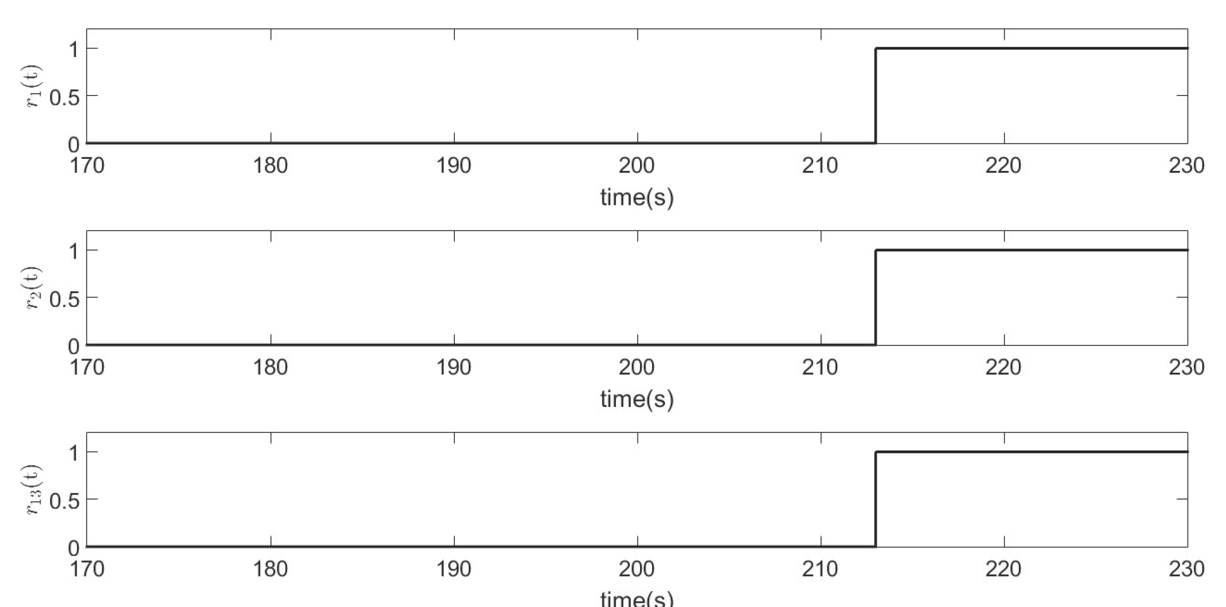
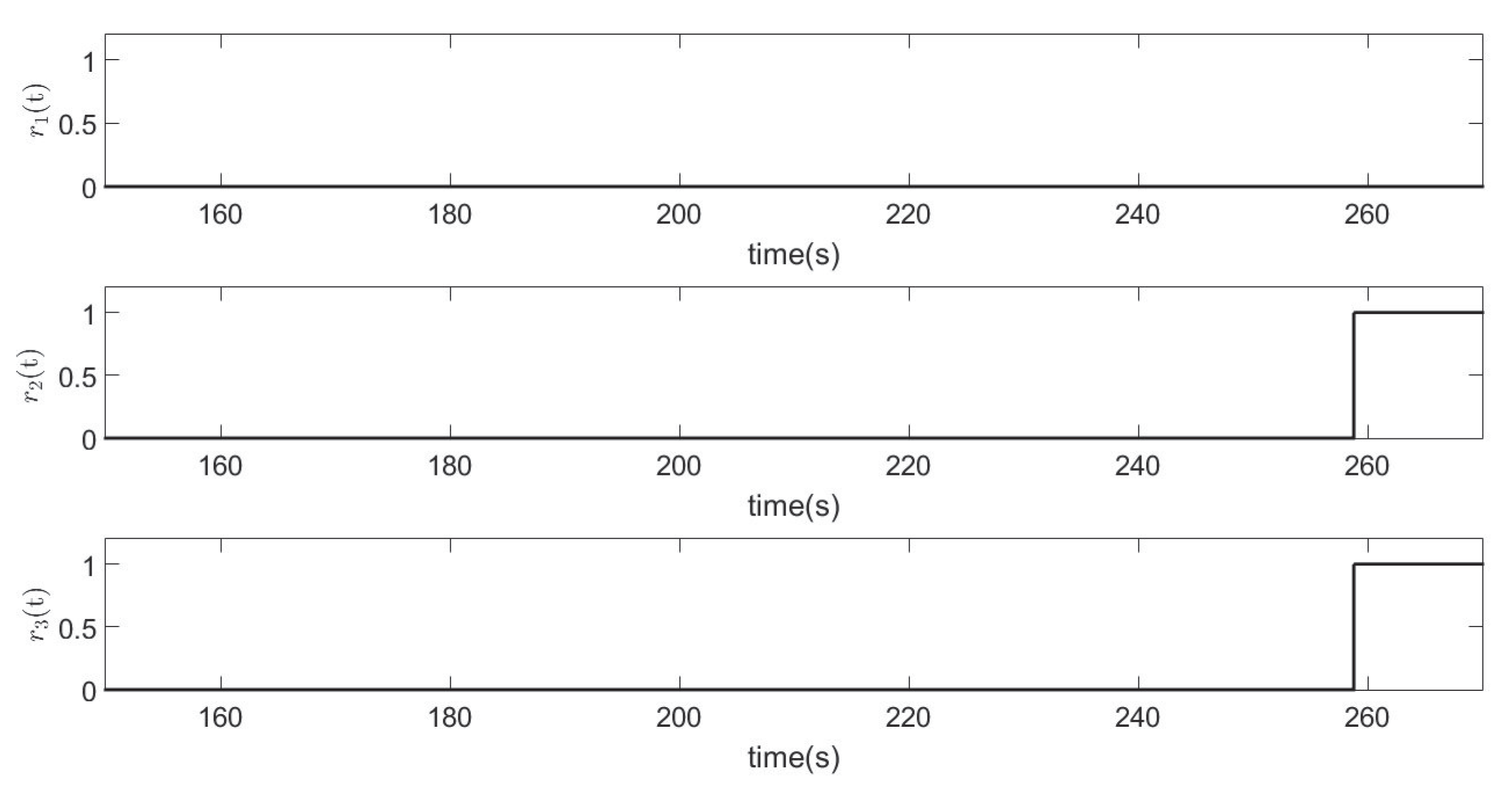
After a residual generator is designed. It should be implemented to obtain the signals, called residuals, that will be used to get the information about the faults. Ideally, the residuals are zero if no faults are present and only different from zero when a fault is present. In practical situations, however, the residual will not be zero because of model uncertainty of small perturbations. In order to avoid false alarms a residual evaluation procedure is included. The idea is to use the obtained signals (residuals) as an argument of a function. for simplicity, a memory-less function is used which make the residual positive. In this paper an absolute value function is utilized. The result of the absolute value is compared to a (fix) threshold. An active residual is declared only when the resulting absolute value of the residual is bigger than the threshold. Otherwise the residual is declared as non-active. The analysis of active/non-active residuals brings us the information if a fault is present and in the case which one is.

When a perturbation and a fault are acting on the same channel, that is called a coupled, and there is no way to distinguish between them using this method. Thus, to be able to distinguish between a perturbation and a specific fault it is required that first, the decoupling approach presented in Section 3.1 produces two different subsystems and, then to design a residual generator for each of them.

4. Study Case

An application example is presented in this section. The system is a laboratory device, a two degree of freedom helicopter of Quanser^®.

4.1. 2-Dof Helicopter

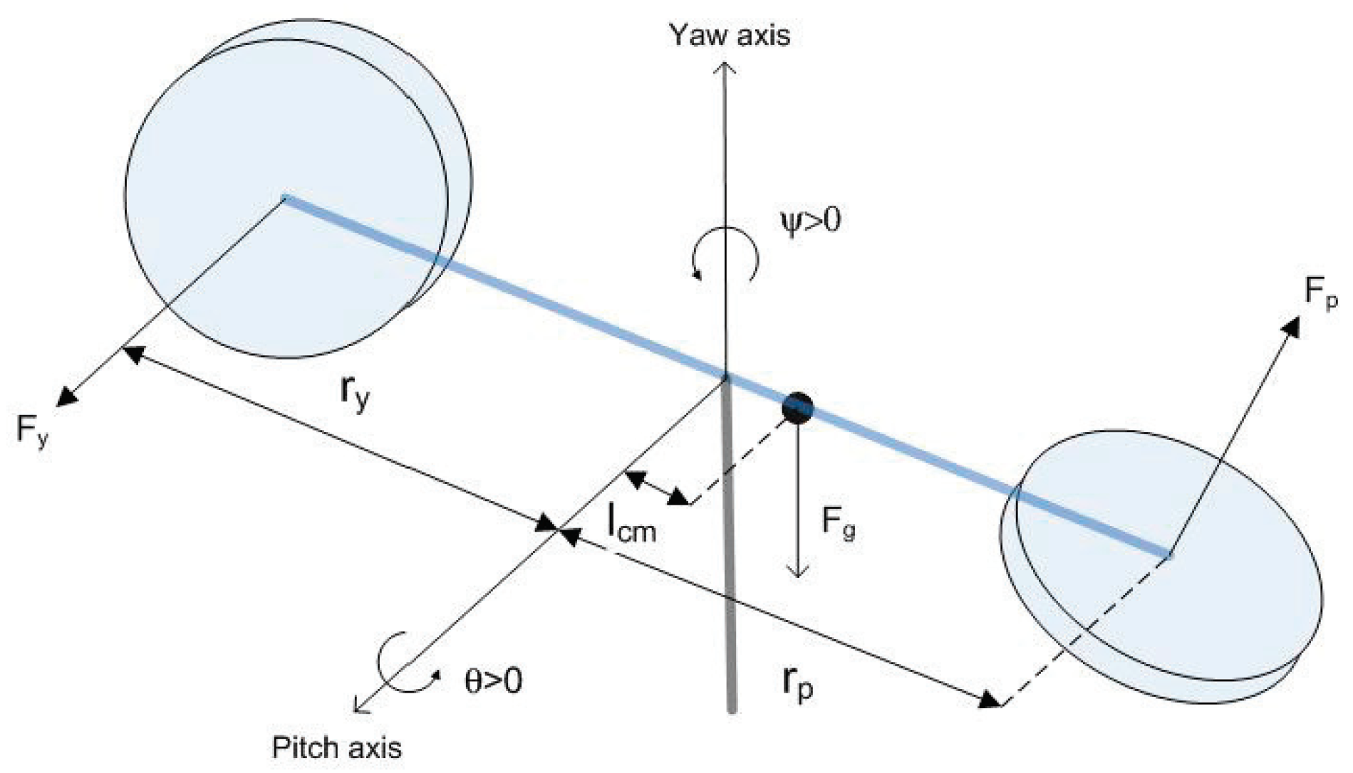
Consider the Quanser^® 2-DOF helicopter, a testing prototype that is on a fixed pedestal (that does the pivot function) and has two motors, one front for lift and one rear or tail for yaw, Figure 2.

The system model can be written in normal way through following nonlinear second order equation, matrix form:

$$D\left(q\right)\ddot{q}+N(q,\dot{q})+g_v\left(q\right)=\tau ,$$

(17)

where $\tau$ is the input vector, $g_v\left(q\right)$ is the vector of gravitational pairs, $D\left(q\right)$ is the inertial matrix, symmetric and positive definite, $N(q,\dot{q})$ models the quadratic effects in velocity generated by centrifugal and Coriolis forces. For the Quanser^® system, it is convenient to define the generalized coordinate vector $q={[\varphi ,\psi ]}^T$, where $\varphi$ and $\psi$ are the pitch and yaw angles. Consider $\tau ={[U_p,U_y]}^T$, and

$$\begin{array}{ccc}\hfill D\left(q\right)& =& \left[\begin{array}{cc}{m}_1{l_1}^2+m_2{l_2}^2& 0\\ 0& m_1{l_1}^2{cos}^2\left(\varphi \right)+m_2{l_2}^2{cos}^2\left(\varphi \right)\end{array}\right],\hfill \\ \hfill g_v\left(q\right)& =& \left[\begin{array}{c}{m}_{1}g{l}_{1}cos\left(\varphi \right)-m_{2}g{l}_{2}cos\left(\varphi \right)\\ 0\end{array}\right].\hfill \end{array}$$

4.2. Hamiltonian Representation

Similar to ref. [28], consider the generalized moment $p\left(t\right)$, defined by

$$p=D\left(q\right)\dot{q},$$

(18)

and the Hamiltonian function

$$\mathcal{H}(q,p)=\frac{1}{2}{p}^T{D}^{-1}\left(q\right)p+U\left(q\right),$$

(19)

where $U\left(q\right)$ represents the potential energy of system. Thus, the system (17) can be written as

$$\begin{array}{ccc}\hfill \dot{q}& =& \frac{\partial \mathcal{H}(q,p)}{\partial p}=D^{-1}\left(q\right)p,\hfill \end{array}$$

(20)

$$\begin{array}{ccc}\hfill \dot{p}& =& -\frac{\partial \mathcal{H}(q,p)}{\partial q}+\tau ,\hfill \end{array}$$

(21)

$$\begin{array}{ccc}\hfill \dot{p}& =& -\frac{\partial }{\partial q}\left(\frac{1}{2}{p}^T{D}^{-1}\left(q\right)p\right)-\frac{\partial }{\partial q}U\left(q\right)+\tau ,\hfill \end{array}$$

(22)

where $\frac{\partial }{\partial q}U\left(q\right)=g_v\left(q\right)$.

Equations that represent dynamics of system are the following:

$$\begin{array}{ccc}\hfill {\dot{x}}_1& =& \frac{x_3}{l^2(m_1+m_2)},\hfill \end{array}$$

(23)

$$\begin{array}{ccc}\hfill {\dot{x}}_2& =& \frac{x_4}{l^2{cos}^2\left(x_1\right)(m_1+m_2)},\hfill \end{array}$$

(24)

$$\begin{array}{ccc}\hfill {\dot{x}}_3& =& \frac{-x_4^{2}sin\left(x_1\right)}{l^2{cos}^3\left(x_1\right)(m_1+m_2)}-glcos\left(x_1\right)(m_1-m_2)+U_p,\hfill \end{array}$$

(25)

$$\begin{array}{ccc}\hfill {\dot{x}}_4& =& U_y,\hfill \end{array}$$

(26)

for $x^T=\left[x_1{x}_2{x}_3{x}_4\right]$ the state vector with $x_1=\varphi$, $x_2=\psi$, $x_3=\dot{\varphi }$ and $x_4=\dot{\psi }$. It is important to mention that the control law $\tau ={[U_p,U_y]}^T$ used to stabilize the closed loop control system is a PD type controller that was tuned using the method presented in ref. [31].

Table 1. Parameters used in the equations.

Parameter	Description
$x_1$$\left(\varphi \right)$	Pitch angle
$x_2$$\left(\psi \right)$	Yaw angle
$x_3$$\left(\dot{\varphi }\right)$	Pitch angular velocity
$x_4$$\left(\dot{\psi }\right)$	Yaw angular velocity
$Up$	Pitch control input
$Uy$	Yaw control input
$m_1$	Mass of lift motor
$m_2$	Mass of tail motor
$1_1$	Length $m_1$ to center of mass
$1_2$	Length $m_2$ to center of mass
g	Gravity

shows the description of the parameters used in the previous equations.

Now, considering the generalized Hamiltonian function

$$H=\frac{1}{2}{x}^{T}x,$$

(27)

with $M=I_{4\times 4}$, starting of (3), results the generalized Hamiltonian function

$$\begin{array}{ccc}\hfill \dot{x}& =& J\left(x\right)\frac{\partial H\left(x\right)}{\partial x}+S\left(x\right)\frac{\partial H\left(x\right)}{\partial x}+F\left(x\right)+G\underset{u}{\underbrace{\left[\begin{array}{c}{U}_p\\ U_y\end{array}\right]}},\hfill \end{array}$$

(28)

$$\begin{array}{ccc}\hfill y& =& C\frac{\partial H\left(x\right)}{\partial x},\hfill \end{array}$$

(29)

where,

$$\begin{array}{ccc}\hfill \frac{\partial H}{\partial x}& =& x,\hfill \\ \hfill J\left(x\right)& =& \left[0\right]\in {\mathbb{R}}^{4x4},\hfill \\ \hfill S\left(x\right)& =& \left[0\right]\in {\mathbb{R}}^{4x4},\hfill \\ \hfill F\left(x\right)& =& \left[\begin{array}{c}\frac{x_3}{l^2(m_1+m_2)}\\ \frac{x_4}{l^2{cos}^2\left(x_1\right)(m_1+m_2)}\\ \begin{array}{c}\frac{-x_4^{2}sin\left(x_1\right)}{l^2{cos}^3\left(x_1\right)(m_1+m_2)}-glcos\left(x_1\right)(m_1-m_2)\\ 0\end{array}\end{array}\right],\hfill \\ \hfill G& =& \left[\begin{array}{cc}0& 0\\ 0& 0\\ 1& 0\\ 0& 1\end{array}\right]\hfill \end{array}$$

with

$$C=\left[\begin{array}{cccc}1& 0& 0& 0\\ 0& 1& 0& 0\end{array}\right].$$

(30)

4.3. Fault Modeling

For this system, four possible faults are considered, one for each sensor and one for each actuator. The faults could be additive or multiplicative, in this paper, we focus on the case of additive faults, which are modeled as exogenous inputs to the system. The faults can be incipient, abrupt or intermittent, depending on the form in which the faults are manifested, see refs. [1,2,3].

4.3.1. Additive Faults Representation

The additive faults are modeled with inputs in the actuators channel $f_{ai}$, as well as in the output channel $f_{si}$, with $i=1,2,3$. This corresponds to

$$\begin{array}{ccc}\hfill \dot{x}& =& J\left(x\right)\frac{\partial H\left(x\right)}{\partial x}+S\left(x\right)\frac{\partial H\left(x\right)}{\partial x}+F\left(x\right)+Gu+E_f\left[\begin{array}{c}{f}_{a1}\\ f_{a2}\end{array}\right],\hfill \end{array}$$

(31)

$$\begin{array}{ccc}\hfill y& =& C\frac{\partial H\left(x\right)}{\partial x}+\left[\begin{array}{c}{f}_{s1}\\ f_{s2}\end{array}\right],\hfill \end{array}$$

(32)

where

$$E_f=\left[\begin{array}{cc}0& 0\\ 0& 0\\ 1& 0\\ 0& 1\end{array}\right].$$

(33)

4.3.2. Fault Decoupling

Sensor Faults

In the case of sensor faults, only one sensor is considered as output. So, a residual is generated through the corresponding observer in the observable part of the system. For this case, the sensor faults, an observer of complete order is considered. The output estimation error will be used as a residual. Thus two residuals are obtained, one for each sensor.

Subsystem 1. For the first sensor, we consider the subsystem formed by the following equations, assuming that $x_2$ is free of fault:

$$\begin{array}{ccc}\hfill {\dot{x}}_1& =& \frac{x_3}{l^2(m_1+m_2)},\hfill \end{array}$$

(34)

$$\begin{array}{ccc}\hfill {\dot{x}}_3& =& \frac{-x_4^{2}sin\left(x_1\right)}{l^2{cos}^3\left(x_1\right)(m_1+m_2)}-glcos\left(x_1\right)(m_1-m_2)+U_p,\hfill \end{array}$$

(35)

$$\begin{array}{ccc}\hfill {\dot{x}}_4& =& U_y,\hfill \end{array}$$

(36)

$$\begin{array}{ccc}\hfill y_{s1}& =& x_1\hfill \end{array}$$

(37)

Subsystem 2. For the second subsystem we assume that $x_1$ is free of fault, the following equations form the second subsystem:

$$\begin{array}{ccc}\hfill {\dot{x}}_2& =& \frac{x_4}{l^2{cos}^2\left(x_1\right)(m_1+m_2)},\hfill \end{array}$$

(38)

$$\begin{array}{ccc}\hfill {\dot{x}}_4& =& U_y,\hfill \end{array}$$

(39)

$$\begin{array}{ccc}\hfill y_{s2}& =& x_2\hfill \end{array}$$

(40)

Actuator Faults

Similar to the case of sensor faults, we obtained the decoupled subsystems that are sensitive only to one particular fault, in this way, the residual is generated from an observer based on output feedback.

Subsystem 3. For the first actuator fault ($f_{a1}$), the residual occurs in the channel of $U_p$ since $x_1$ is known, and assuming that $x_2$ is free of fault.

$$\begin{array}{ccc}\hfill {\dot{x}}_1& =& \frac{x_3}{l^2(m_1+m_2)},\hfill \end{array}$$

(41)

$$\begin{array}{ccc}\hfill {\dot{x}}_3& =& \frac{-{\left({\dot{x}}_2{l}^2{cos}^2\left(x_1\right)(m_1+m_2)\right)}^{2}sin\left(x_1\right)}{l^2{cos}^3\left(x_1\right)(m_1+m_2)}\hfill \end{array}$$

(42)

$$\begin{array}{ccc}& & -glcos\left(x_1\right)(m_1-m_2)+U_p,\hfill \end{array}$$

(43)

$$\begin{array}{ccc}\hfill y_{a1}& =& x_1.\hfill \end{array}$$

(44)

Note that $x_4$ is not available, it can be obtained from the dynamic of the system as:

$$x_4={\dot{x}}_2{l}^2{cos}^2\left(x_1\right)(m_1+m_2).$$

(45)

Subsystem 4. For to appreciate the fault in the second actuator ($f_{a2}$) is considered the following equations.

$$\begin{array}{ccc}\hfill {\dot{x}}_2& =& \frac{x_4}{l^2{cos}^2\left(x_1\right)(m_1+m_2)},\hfill \end{array}$$

(46)

$$\begin{array}{ccc}\hfill {\dot{x}}_4& =& U_y,\hfill \end{array}$$

(47)

$$\begin{array}{ccc}\hfill y_{a2}& =& x_2.\hfill \end{array}$$

(48)

Remark 1.

Note that for fault decoupling an inspection procedure is used instead of a nonlinear transformation, i.e., for sensor i, the output is selected (omitting all other outputs) as well as all differential equations associated with the states that explicitly appear in the selected output and the ones required to complete the states present in the differential equations selected.

Remark 2.

The subsystem for sensor fault 2 and actuator 2 is the same, so only one will be used.

4.4. Residual Design

The observer-based residuals are built following the method presented in Section 3.

For the construction of the residual generator sensible to sensor fault 1, we considered the first subsystem:

$$\begin{array}{ccc}\hfill {\dot{x}}_1& =& \frac{x_3}{l^2(m_1+m_2)},\hfill \end{array}$$

(49)

$$\begin{array}{ccc}\hfill {\dot{x}}_3& =& \frac{-x_4^{2}sin\left(x_1\right)}{l^2{cos}^3\left(x_1\right)(m_1+m_2)}-glcos\left(x_1\right)(m_1-m_2)+U_p,\hfill \end{array}$$

(50)

$$\begin{array}{ccc}\hfill {\dot{x}}_4& =& U_y,\hfill \end{array}$$

(51)

$$\begin{array}{ccc}\hfill y_{s1}& =& x_1,\hfill \end{array}$$

(52)

it leads to its generalized Hamiltonian representation, with

$$\frac{\partial H}{\partial x}={\left[x_1{x}_3{x}_4\right]}^T.$$

(53)

In this mode, we have to:

$$\begin{array}{ccc}\hfill J\left(x\right)& =& \left[0\right]\in {\mathbb{R}}^{3x3},\hfill \end{array}$$

(54)

$$\begin{array}{ccc}\hfill S\left(x\right)& =& \left[0\right]\in {\mathbb{R}}^{3x3},\hfill \end{array}$$

(55)

$$\begin{array}{ccc}\hfill F\left(x\right)& =& \left[\begin{array}{c}\frac{x_3}{l^2(m_1+m_2)}\\ \begin{array}{c}\frac{-x_4^{2}sin\left(x_1\right)}{l^2{cos}^3\left(x_1\right)(m_1+m_2)}-glcos\left(x_1\right)(m_1-m_2)\\ 0\end{array}\end{array}\right],\hfill \end{array}$$

(56)

$$\begin{array}{ccc}\hfill G& =& \left[\begin{array}{cc}\begin{array}{c}0\\ \begin{array}{c}1\\ 0\end{array}\end{array}& \begin{array}{c}0\\ \begin{array}{c}0\\ 1\end{array}\end{array}\end{array}\right],\hfill \end{array}$$

(57)

$$\begin{array}{ccc}\hfill C& =& \left[\begin{array}{ccc}1& 0& 0\end{array}\right]\hfill \end{array}$$

(58)

The pair $(C,S)$ is detectable agree with the definition 2.1 in ref. [27] since the matrix $\left[\begin{array}{c}C\\ \lambda I_{3\times 3}-S\end{array}\right]$ is of full rank for any value of $\lambda$ in ${\mathbb{Z}}_{<0}=\{\overline{\lambda }\in \mathbb{Z}:\Re \left\{\overline{\lambda }\right\}<0\}$. So, the residual is defined from the observer,

$$\begin{array}{ccc}\hfill {\dot{\widehat{x}}}_1& =& \frac{{\widehat{x}}_3}{l^2(m_1+m_2)}+L_1(y_1-{\widehat{x}}_1),\hfill \\ \hfill {\dot{\widehat{x}}}_3& =& \frac{-{\widehat{x}}_4^{2}sin\left(x_1\right)}{l^2{cos}^3\left(x_1\right)(m_1+m_2)}-glcos\left(x_1\right)(m_1-m_2)+U_p,\hfill \\ \hfill {\dot{\widehat{x}}}_4& =& U_y,\hfill \\ \hfill {\widehat{y}}_{s1}& =& {\widehat{x}}_1\hfill \end{array}$$

Note that the residual is designed from a copy of the original subsystem and the correction factor $L_1(y_1-{\widehat{y}}_1)$.

For the fault in the second sensor $\left(f_{s2}\right)$, and the faults in the two actuators $\left(f_{a1}\right)$ and $\left(f_{a2}\right)$, the decoupling is similar to the procedure utilized in the fault $\left(f_{s1}\right)$. In

Table 2. Sensitivity of residuals with respect to faults.

	RESUDIAL
FAULT	${\mathit{r}}_{\mathbf{1}}$	${\mathit{r}}_{\mathbf{2}}$	${\mathit{r}}_{\mathbf{3}}$	${\mathit{r}}_{\mathbf{4}}$
$f_{s1}$	√	√	√	√
$f_{s2}$		√	√	√
$f_{a1}$	√		√
$f_{a2}$	√	√		√

, a summary of the sensitivity of each one of the different faults is presented, where √ means that the subsystem is sensitive to the corresponding fault.

In the table we can to see that the subsystem 2 and 4 have the same sensitivity to the faults $f_{s1},f_{s2},f_{a2}$, therefore, one of them does not provide additional information. The four residuals are obtained assuming that only one fault at a time is present, and not all of them simultaneously. A residual is obtained by considering a derivative in time, so obtaining this derivative could be a difficult task in the presence of noise. It is important to notice that the generation of residuals based on observers constitutes a reliable option to reduce noisy effects, by virtue of the inherent filtering characteristic of the observer, see ref. [24].

The considered design allows us to isolate all single faults. However, when more than one simultaneous fault is present, an alarm can be activated, but we cannot know which faults are involved.

5. Results

Two types of results are provided in this section. First, simulation results are used to verify the designed fault isolation schema. After, an experimental laboratory device is used to implement the designed residuals. Two types of faults are considered, actuator and sensor faults.

5.1. Fault Scenaries

Two additive actuator faults and two additive sensor faults are considered. The different considered cases are presented in

Table 3. Cases considered.

Case	Description
1	Nominal behaviour, without faults
2	fault in sensor 1
3	fault in sensor 2
4	fault in actuator 1
5	fault in actuator 2

.

5.2. Simulation Results

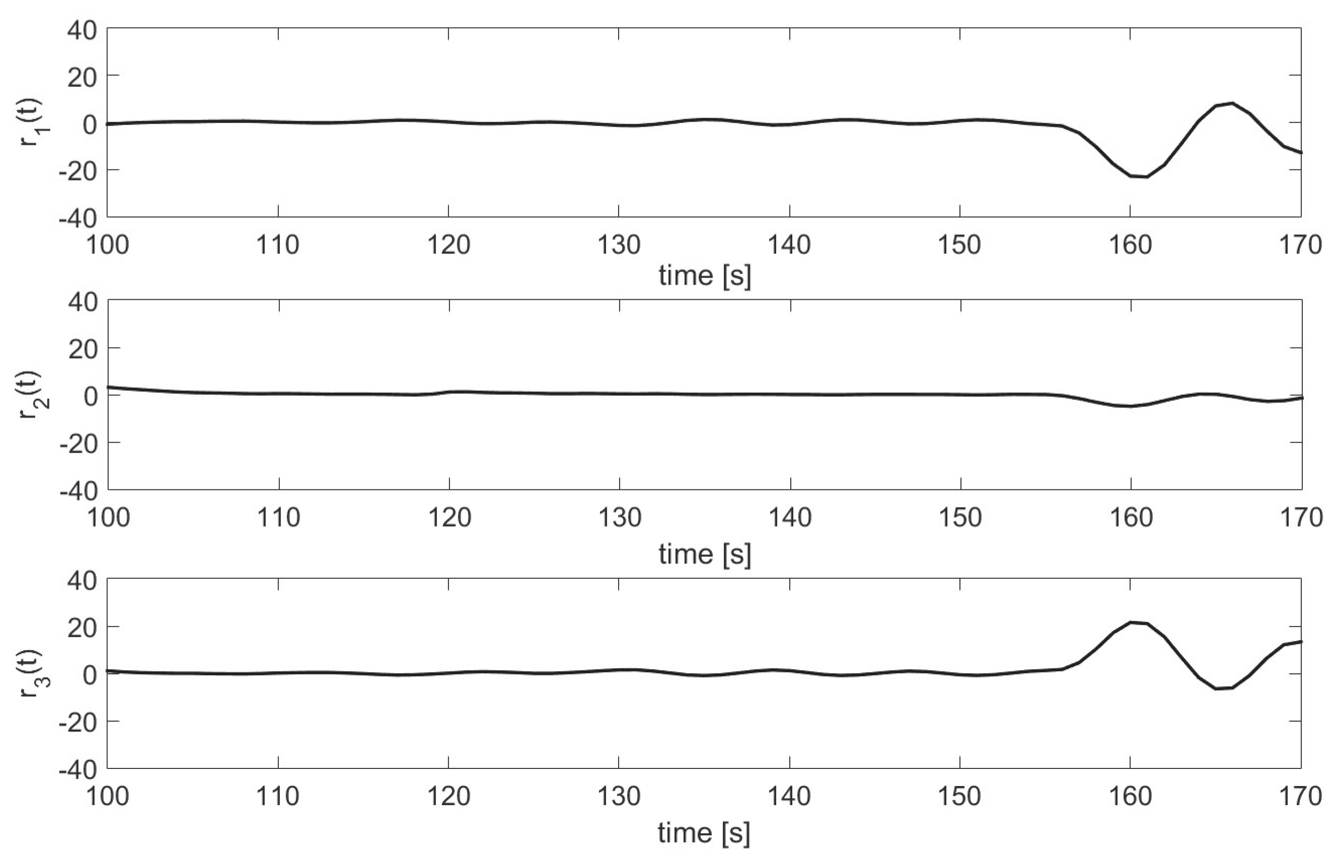
The simulation was performed in Simulink to MATLAB^®. The parameters shown in

Table 4. Parameters used in the simulation results.

Parameter	Description	Value
$m_1$	Mass of lift motor	$0.014$ kg
$m_2$	Mass of tail motor	$0.232$ kg
$1_1$	Length $m_1$ to center of mass	$0.203$ m
$1_2$	Length $m_2$ to center of mass	$0.203$ m
g	Gravity	$9.8$ m/s${}^2$

were obtained from the actual 2-DOF helicopter of Quanser^® and those were used to obtain the simulation results shown in Figure 3 and Figure 4.

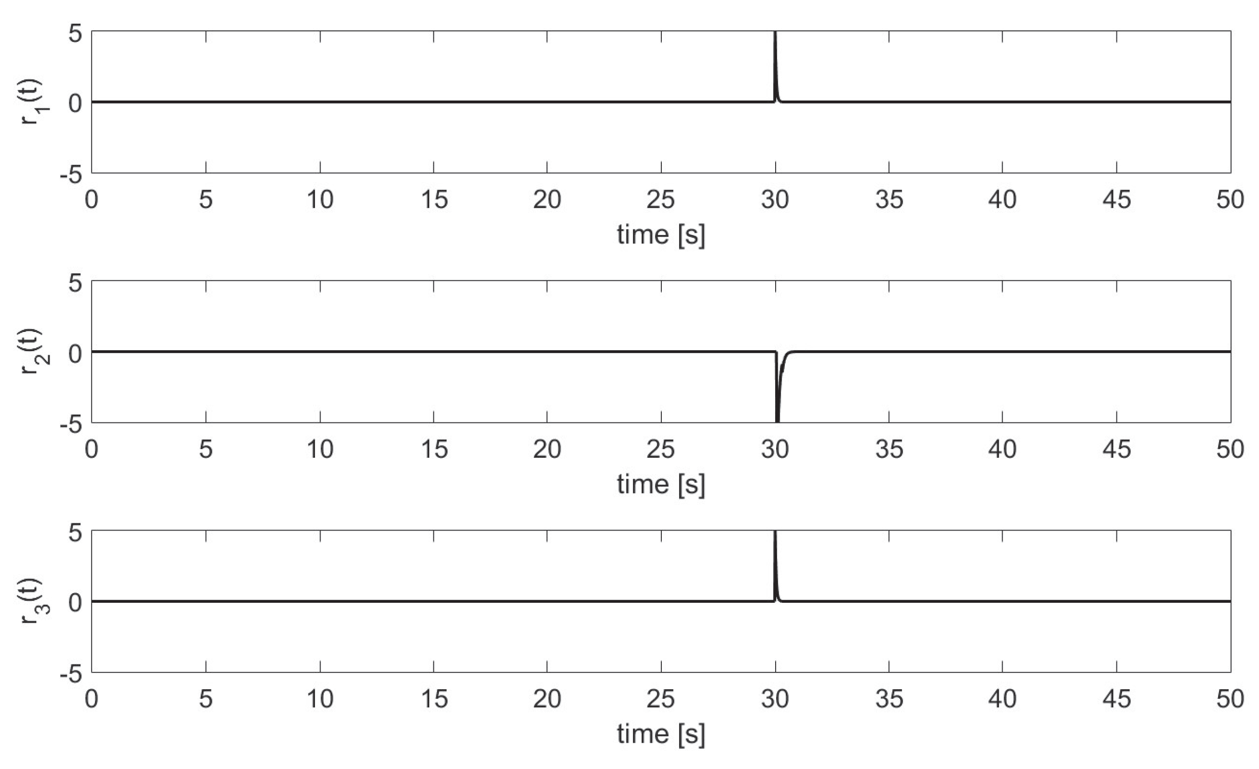
Sensor Fault 1. Figure 3 shows the behavior of the residuals when the fault $f_{s1}$ is present. When the fault $f_{s1}$ occurs, all three residuals present sensitivity to the fault; this can be noticed because they are different from zero, indicating they are sensitive to the fault.

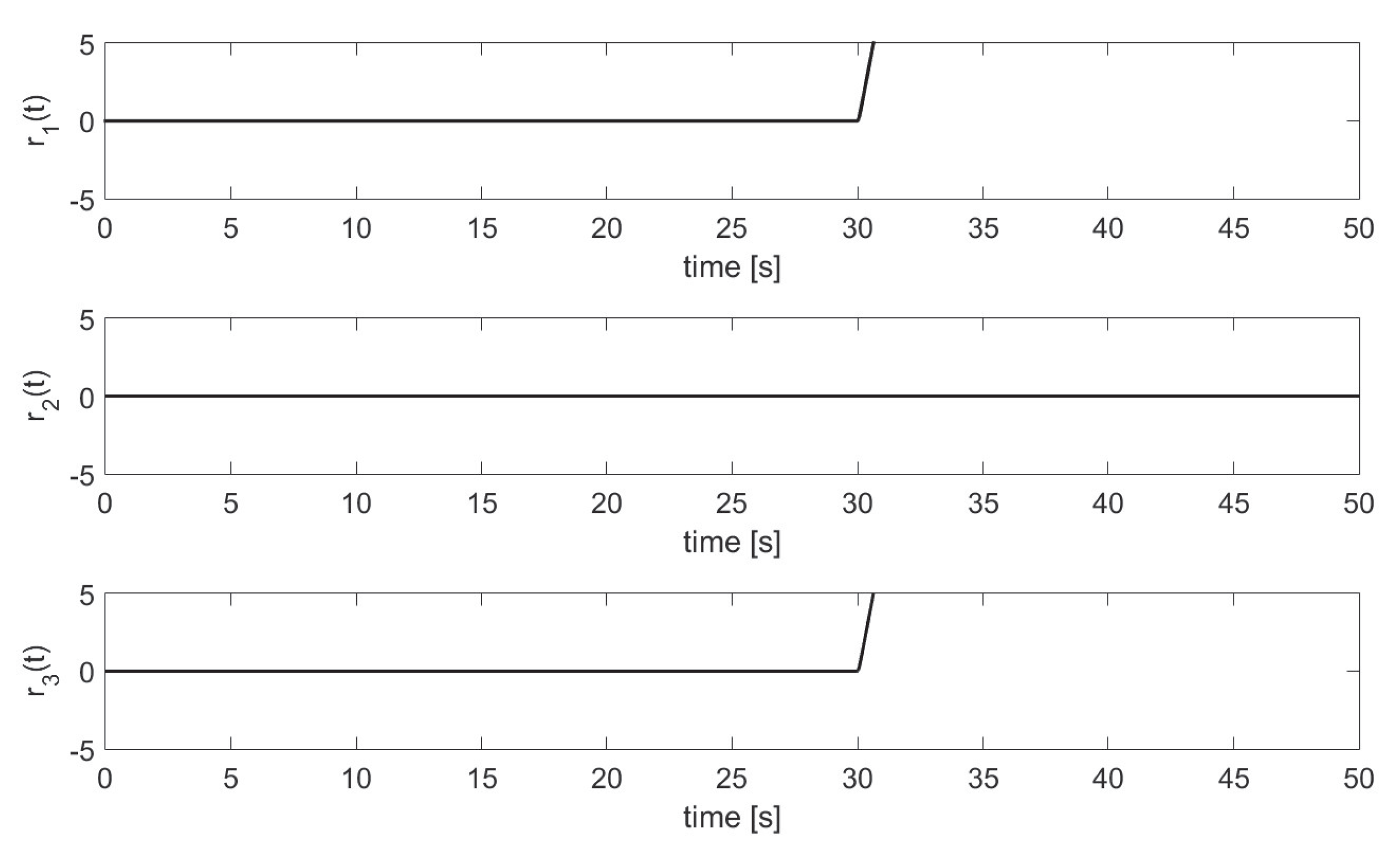
Actuator Fault 1. Figure 4 shows the behavior of the residuals when the fault $f_{a1}$ is present. As can be noticed, the residuals $r_1$ and $r_3$ respond to this fault because are differ from zero indicating sensitivity to the fault, while the residual $r_2$ is zero at all times, due its insensitivity to the fault.

5.3. Experimental Results

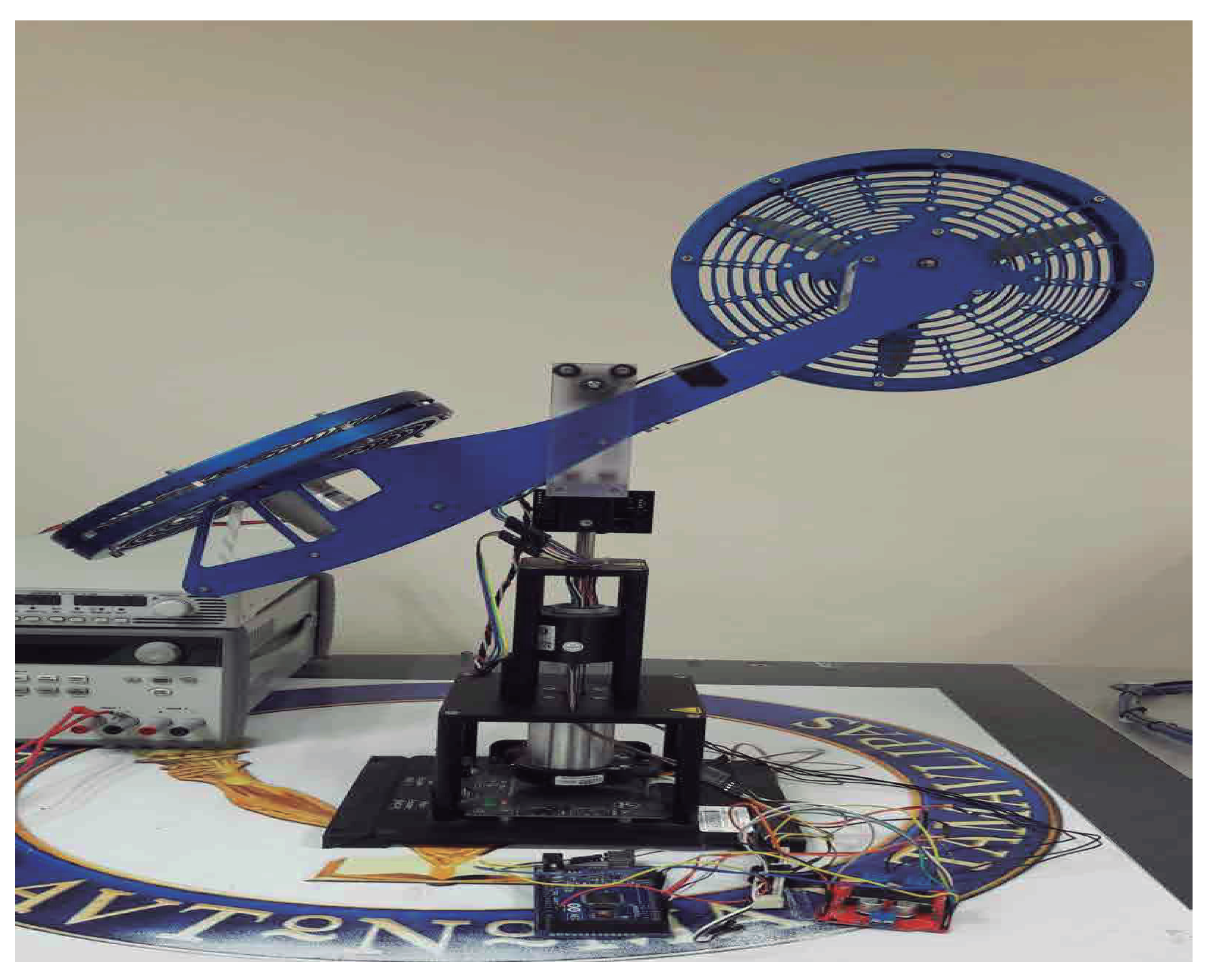
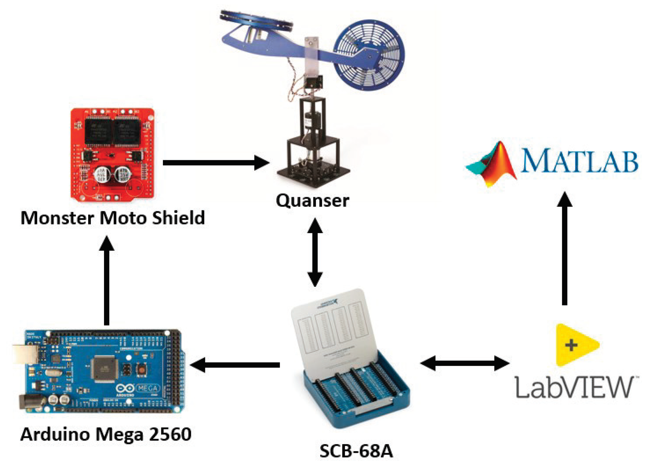
To validate the proposed scheme, a test on a physical real-time helicopter was performed. The experimental platform shown in Figure 5 and its corresponding schematic diagram in Figure 6 which shows the communication and data directly between the devices and the software. First of all, it is necessary to control the system to carry out the detection of faults. Because the 2-DOF system is in a closed loop, is possible to implement a PID control. The experimental platform consists of two motors, a lift motor that causes the pitch motion, and a tail motor, which produces the yaw motion. DC motors with a nominal voltage of 12 volts. The platform parameters are shown in Table 4. The Labview software was used as a programming platform, it contains the control law to stabilize the system and the algorithm to fault diagnosis; the SCB-68A board from National Instrumens^® and an Arduino^® Mega 2560 board with 56 input/output pins were used as an interface for communication between the physical system and the software. For the power part, a SparkFun^® Monster Moto Shield H-bridge was used with a voltage capacity of 16 volts, 30 amps of current and 20 KHz of PWM frequency. The sensing was carried out by two rotary optical encoders, one placed at the base of the platform, which allows the yaw angle to be measured, $\psi$, and the other placed in the center of the platform which measures pitch angle $\varphi$.

The information of the angles and angular velocities of pitch and yaw are obtained through the SCB-68A board, the fault detection and control algorithm processes the information and feeds back the controlled signal to the interface consisting of two devices, the SCB-68A board and the Arduino^® Mega 2560, which transforms the signal to PWM; taking the PWM signal as input, the power device supplies the motors with voltage. The data acquired is processed in the Matlab^® software to obtain the graphs of the behavior of the residuals.

To produce faults in the physical system, external signals to the system were injected into both sensors and actuators, one at a time. Is important to mention that the produced faults in each of the physical tests, were in a proportion of 50% with respect to the output.

The threshold of the normalized residual evaluation is presented in each of the cases in which the faults occur. The threshold for sensor failure is $\pm 5$ and the threshold for actuators failure is $\pm 10$, these values were chosen based on the structure and dynamics of the decoupled equations.

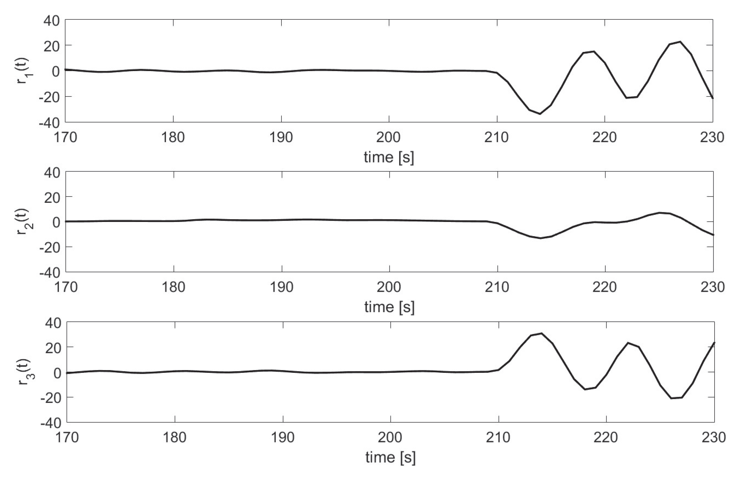
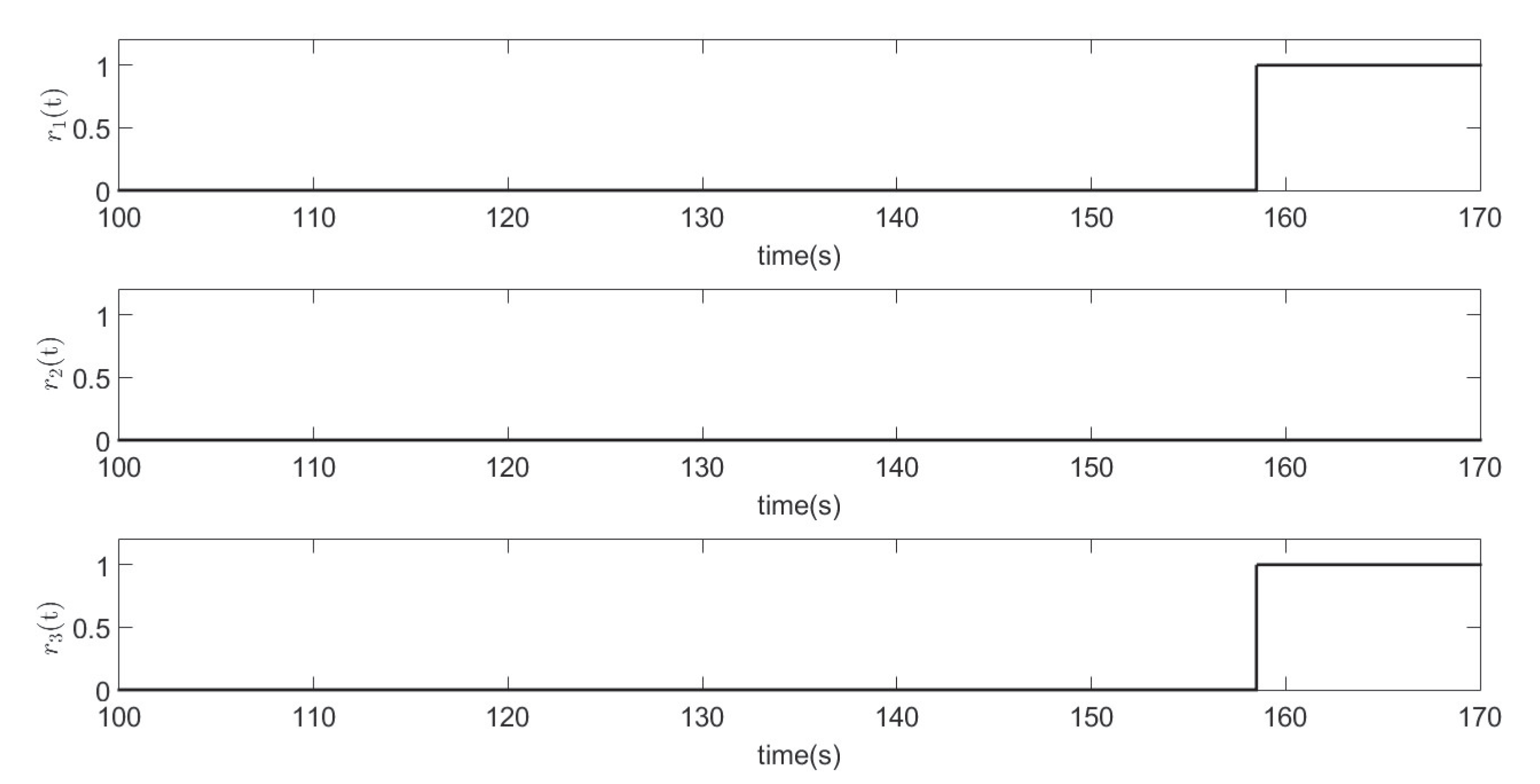
Sensor Fault 1. Figure 7 and Figure 8 show the response of the residuals to the sensor fault $f_{s1}$, where the residuals that differ from zero indicate sensitivity to the fault. According to the signature table, all residues response to the fault.

Sensor Fault 2. Figure 9 and Figure 10 show the response of the residuals to the sensor fault $f_{s2}$. As can be noticed, in the case when a fault in sensor two exists, the residuals $r_2$ and $r_3$ differ from zero, indicating sensitivity to the fault.

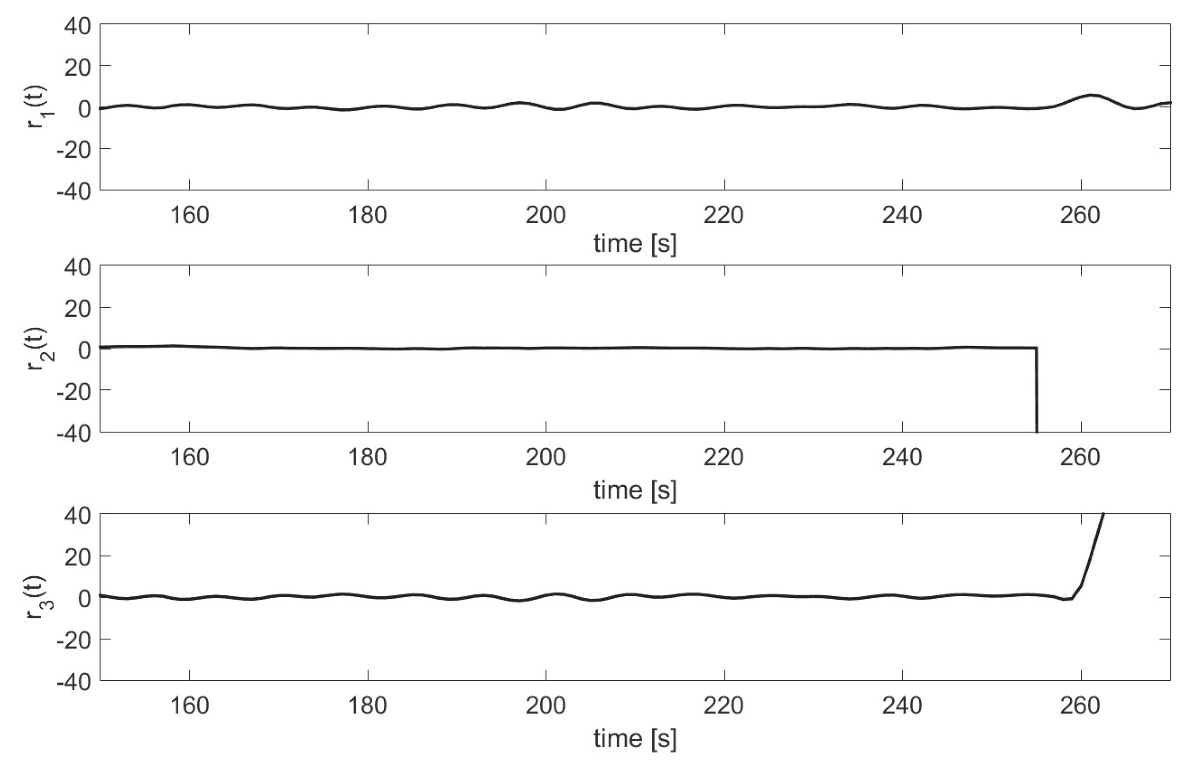
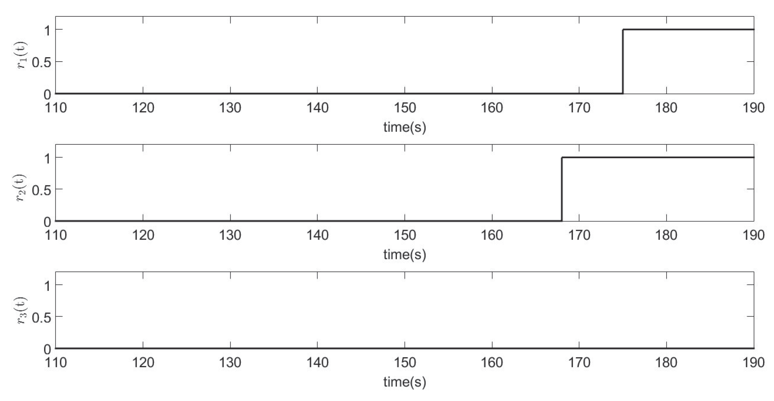
Actuator Fault 1. Figure 11 and Figure 12 show the response of the three residuals when the actuator fault $f_{a1}$ is present. Note that the fault effects on residuals 1 and 3 occur when they are different from zero, due to their sensitivity to the fault.

Actuator Fault 2. Figure 13 and Figure 14 show the response to residual to the actuator fault $f_{a2}$. Where the residuals $r_1$ and $r_2$ response to this fault. The residuals are different from zero, indicating sensitivity to the fault while the $r_3$ remains very close to zero indicating insensitivity to the fault.

5.4. Discussion

Due to the structure and dynamics of the system under study, a state-coupling is presented; this exposes an important complication for fault detection. The problem is attacked by decoupling each fault, thus ensuring that each residual generated is sensitive to a specific fault. We can observe that when a fault occurs in sensor 1, according to Table 2 of sensitivity of the residuals with respect to the fault, this must be manifested in all the residues. However, we can see in Figure 7, which shows the behavior of the residues sensitive to this fault, which shows the behavior of the residues sensitive to this fault, that the residual 2 presents a tenuous response compared to residual $r_1$ and $r_3$; this could be confused with the behavior of the residuals of actuator 1 as shown in Figure 11. However, observing the scale of the residuals, it is easy to distinguish when any of the two faults are present, since the residual $r_2$ in the presence of the fault in sensor 1 shows a greater magnitude, than compared to the $r_2$ in the presence of the fault on actuator 1 is very small in magnitude that we can say it is zero.

The experimentation data were obtained through the LabView software, and to show the experimentation data, the graphs were performed in the Matlab software. The difference in the time scale between the presented simulation and the experimentation graphs is due to the time it takes to adjust the sensor (encoder). In the simulation graphs, once the algorithm has started, the data begins to be recorded; therefore, the time starts at zero. However, in each new test performed during the experimentation was necessary to establish the zeros of the angles (pitch, yaw), which takes more than a minute; therefore, the time in the graph does not start at zero.

6. Conclusions

For a wide range of dynamic systems, which admit a Hamiltonian representation, it is possible to apply a systematic fault detection procedure in order to detect and isolate a set of faults. The results are not dependent on a specific controller (in the case of closed-loop controlled system). Further, in order to design fault-specific residuals (residuals sensible to a specific fault or a subset of faults) nonlinear decoupling is used. This decoupling procedure can be also used to look for a decoupling of perturbations too. In order to avoid false alarms, an evaluation function and a threshold is used with the obtained residual. The fault signature matrix, obtained as a result of the decoupling and residual generation will be used to associate a specific fault to the behavior of the residual (active for specific faults and inactive for the rest of faults (or perturbations). The fault isolation results have been tested on a laboratory test facility of a 2-DOF helicopter. An experimental test shows the effectiveness of the proposed approach. Some problems associated with physical implementation have been solved. Non-permanent fault has been used in the experimental setup. Future work includes the search for minimum fault sizes that can be detected (optimize for small faults). The time for detection should be reduced as well as the consideration of additional information in order to isolate structural-coupled faults (or perturbations) as the sign of residuals of patterns in them. Another topic that could be addressed as future work is developing control algorithms that take into account the failure reconfiguration to get a fault-tolerant control system.

References

1. Isermann, R. Fault-Diagnosis Applications: Model-Based Condition Monitoring: Actuators, Drives, Machinery, Plants, Sensors, and Fault-Tolerant Systems; Springer Science & Business Media: Berlin, Germany, 2011. [Google Scholar]
2. Chen, J.; Patton, R. Robust Model-based Fault Diagnosis for Dynamic Systems; Springer Science & Business Media: Boston, MA, USA, 1999. [Google Scholar]
3. Ding, S. Model-Based Fault Diagnosis Techniques: Design Schemes, Algorithms, and Tools; Springer Science & Business Media: Berlin, Germany, 2008. [Google Scholar]
4. Ding, S. Data-Driven Design of Fault Diagnosis and Fault-Tolerant Control Systems; Springer Science & Business Media: London, UK, 2014. [Google Scholar]
5. Alcorta-García, E.; Frank, P.M. Deterministic nonlinear observer-based approaches to fault diagnosis: A survey. Control. Eng. Pract. 1997, 5, 663–670. [Google Scholar] [CrossRef]
6. Bokor, J.; Szabó, Z. Fault detection and isolation in nonlinear systems. Annu. Rev. Control. 2009, 33, 113–123. [Google Scholar] [CrossRef]
7. de Persis, C.; Isidori, A. A geometric approach to nonlinear fault detection and isolation. IEEE Trans. Autom. Control. 2001, 46, 853–865. [Google Scholar] [CrossRef] [Green Version]
8. Seliger, R.; Frank, P.M. Fault-diagnosis by disturbance decoupled nonlinear observers. In Proceedings of the 30th IEEE Conference on Decision and Control, Brighton, UK, 11–13 December 1991; pp. 2248–2253. [Google Scholar]
9. Calado, J.M.; Korbicz, J.; Patan, K.; Patton, R.J.; da Costa, J.M.S. Soft Computing Approaches to Fault Diagnosis for Dynamic Systems. Eur. J. Control 2001, 7, 248–286. [Google Scholar] [CrossRef]
10. Duan, G.; Patton, R. Robust fault detection using Luenberger-type unknown input observers-a parametric approach. Int. J. Syst. Sci. 2001, 32, 533–540. [Google Scholar] [CrossRef]
11. Edwards, C.; Spurgeon, S.; Patton, R. Sliding mode observers for fault detection and isolation. Automatica 2000, 36, 541–553. [Google Scholar] [CrossRef]
12. Venkatasubramanian, V.; Rengaswamy, R.; Yin, K.; Kavuri, S. A review of process fault detection and diagnosis: Part I: Quantitative model-based methods. Comput. Chem. Eng. 2003, 27, 293–311. [Google Scholar] [CrossRef]
13. Jiang, B.; Staroswiecki, M.; Cocquempot, V. Fault estimation in nonlinear uncertain systems using robust/sliding-mode observers. IEEE Control Theory Appl. 2004, 151, 29–37. [Google Scholar] [CrossRef]
14. Han, J.; Yang, Z.; Zhang, Q.; Chen, C.; Li, H.; Lai, S.; Hu, G.; Xu, C.; Xu, H.; Wang, D.; et al. A Method of Insulator Faults Detection in Aerial Images for High-Voltage Transmission Lines Inspection. Appl. Sci. 2019, 9, 9. [Google Scholar] [CrossRef] [Green Version]
15. Raza, A.; Benrabah, A.; Alquthami, T.; Muhammad, A. A Review of Fault Diagnosing Methods in Power Transmission Systems. Appl. Sci. 2020, 10, 1312. [Google Scholar] [CrossRef] [Green Version]
16. Fawwas, D.Z.; Chung, S.H. Adaptive Real-Time and Robust Hydraulic System Fault Detection via Edge Computing. Appl. Sci. 2020, 10, 5933. [Google Scholar] [CrossRef]
17. Dang, S.; Kong, Z.; Peng, L.; Ji, Y.; Zhang, Y. Adaptive State Observer for Robot Manipulators Diagnostics and Health Degree Assessment. Appl. Sci. 2020, 10, 514. [Google Scholar] [CrossRef] [Green Version]
18. Lien, Y.H.; Peng, C.C.; Chen, Y.H. Adaptive Observer-Based Fault Detection and Fault-Tolerant Control of Quadrotors under Rotor Failure Conditions. Appl. Sci. 2020, 10, 3503. [Google Scholar] [CrossRef]
19. Boukens, M.; Boukabou, A.; Chadli, M. Robust adaptive neural network-based trajectory tracking control approach for nonholonomic electrically driven mobile robots. Robot. Auton. Syst. 2017, 92, 30–40. [Google Scholar] [CrossRef]
20. Boukens, M.; Boukabou, A.; Chadli, M. A real time self-tuning motion controller for mobile robot systems. IEEE/CAA J. Autom. Sin. 2018, 6, 84–96. [Google Scholar] [CrossRef]
21. Heredia, G.; Ollero, A. Detection of Sensor Faults in Small Helicopter UAVs Using Observer/Kalman Filter Identification. Math. Probl. Eng. 2011, 2011, 174618. [Google Scholar] [CrossRef]
22. Guo, R.; Guo, K.; Gan, Q.; Zhang, J.; Dong, J.; Bai, L. Fault Diagnosis for Actuators in a Class of Nonlinear Systems Based on an Adaptive Fault Detection Observer. Math. Probl. Eng. 2016, 2016, 2618534. [Google Scholar] [CrossRef] [Green Version]
23. Rodriguez, L. Control Activo Tolerante A Fallas Para Sistemas Hamiltonianos Convergentes. Ph.D. Thesis, Autonomous University of Nuevo León, San Nicolás de los Garza, Nuevo León, México, 2013. [Google Scholar]
24. Rodríguez, L.; Alcorta-García, E.; Lara, D.; Romero, G. A Hamiltonian approach to fault isolation in a planar vertical take–off and landing aircraft model. Int. J. Appl. Math. Comput. Sci. 2015, 25, 65–76. [Google Scholar] [CrossRef] [Green Version]
25. Li, L.; Chadli, M.; Ding, S.X.; Qiu, J.; Yang, Y. Diagnostic Observer Design for T-S Fuzzy Systems: Application to Real-Time Weighted Fault Detection Approach. IEEE Trans. Fuzzy Syst. 2017, 26, 805–816. [Google Scholar] [CrossRef]
26. Rodriguez, L.; Alcorta-García, E. De la representación de sistemas Euler-Lagrange a la hamiltoniana generalizada. Nova Sci. 2015, 7, 1–23. [Google Scholar] [CrossRef]
27. Sira-Ramírez, H.; Cruz-Hernández, C. Synchronization of chaotic systems: A generalized Hamiltonian systems approach. Int. J. Bifurc. Chaos 2011, 11, 1381–1395. [Google Scholar] [CrossRef]
28. der Schaft, A.V. L2-gain and Passivity Techniques in Nonlinear Control; Springer Science & Business Media: London, UK, 2012. [Google Scholar]
29. Frank, P.M. Fault diagnosis in dynamic systems using analytical and knowledge-based redundancy: A survey. Automatica 1990, 26, 459–474. [Google Scholar] [CrossRef]
30. Wünnenberg, J. Observer-Based Fault Detection in Dynamic Systems. Ph.D. Thesis, University Gesamthochschule-Duisburg, Duisburg, Germany, 1990. [Google Scholar]
31. Romero, G.; Alcorta-García, E.; Lara, D.; Pérez, I.; Betancourt, B.; Ocampo, H. New Method for Tuning Robust Controllers Applied to Robot Manipulators. Int. J. Adv. Robot. Syst. 2012, 9, 1–8. [Google Scholar] [CrossRef] [Green Version]
Figure 1. Fault detection scheme.
Applsci 10 08359 g001
Figure 2. Schematic of the 2-degree of freedom (DOF) helicopter.
Applsci 10 08359 g002
Figure 3. Response of residual to the sensor fault f s 1 .
Applsci 10 08359 g003
Figure 4. Response of residual to the fault f a 1 .
Applsci 10 08359 g004
Figure 5. Actual picture of the 2-DOF helicopter.
Applsci 10 08359 g005
Figure 6. Experimental platform.
Applsci 10 08359 g006
Figure 7. Response of residual to the sensor fault f s 1 .
Applsci 10 08359 g007
Figure 8. Normalized residual evaluation in case 2 (fault at sensor 1, f s 1 ).
Applsci 10 08359 g008
Figure 9. Response of residual to the sensor fault f s 2 .
Applsci 10 08359 g009
Figure 10. Normalized residual evaluation in case 3 (fault at sensor 2, f s 2 ).
Applsci 10 08359 g010
Figure 11. Response of residual to the actuator fault f a 1 .
Applsci 10 08359 g011
Figure 12. Normalized residual evaluation in case 4 (fault at actuator 1, f a 1 ).
Applsci 10 08359 g012
Figure 13. Response of residual to the actuator fault f a 2 .
Applsci 10 08359 g013
Figure 14. Normalized residual evaluation in case 5 (fault at actuator 2, f a 2 ).
Applsci 10 08359 g014