Motion Planning for Mobile Robot with Modified BIT* and MPC

Abstract

In this paper, a mobile robot motion planning method with modified BIT* (batch informed trees) and MPC (Model Predictive Control) is presented. The conventional BIT* was modified here by integrating a stretch method that improves the path points connections, to get a collision-free path more quickly. After getting a reference path, the MPC method is employed to determine the motion at each moment with a given objective function. In the objective function, a repulsive function based on the direction and distance of the obstacles is introduced to avoid the robot being too close to the obstacle, so the safety can be ensured. Simulation results show the good navigation performance of the whole framework in different scenarios.

1. Introduction

Mobile robots are widely used in many kinds of life scenes. Autonomous motion planning is the basis for mobile robots to realize various functions. For example, the logistics robot applied in warehouse should be able to move flexibly and plan the path quickly. Indoor mobile robots need to respond to the environment in time and avoid obstacles quickly. The classic algorithm—artificial potential field [1] can find a collision-free path but it will fall into a local minimum in some cases. Besides, there are two popular categories of path planning algorithm for mobile robot: graph-search and sampling-based. The graph-search method first discretizes the map into a grapgh, and then uses the search strategy to find the path with the least cost. Dijkstra [2] and A* [3] method are the two most commonly used graph-search path planning algorithm.

Sampling-based method is effective to solve the path planning problem for mobile robot. It generates path points by sampling in map rather than discretizing the map. In [4], a probabilistic roadmaps (PRMs) method is introduced. It firstly samples some points in the map and construct a graph by connecting these points with collision-free edges, and then use graph-search algorithm to find a path from start to goal state. In [5], the author proposed a rapidly-exploring random tree (RRT) method. RRT construct a tree that tend to explore from start state to goal state by randomly sampling. As long as there is a path from the starting state to the goal state, RRT can always find a collision-free path as the number of iterations increases. However, in the process of exploring, there are many useless points added to the tree due to the randomness of sampling, and the tree is hard to explore to narrow space so it is difficult to get a path through narrow corridor. To solve the limitation of random sampling, a heuristic function guided method based on RRT is proposed in [6]. RRT-connect builds two random trees that rooted at start state and goal state respectively, and uses greedy strategy on the basis of RRT to speed up the search [7]. It has been demonstrated that the path generated by RRT-based algorithm is suboptimal [8]. However, in RRT-based methods, the sampling points are randomly generated and there are a lot of unnecessary exploring, which leads to the inefficiency.

Based on RRT, a lot of optimal planning algorithms have been developed. RRT* uses a predefined cost function to select the node with the lowest cost as the parent node [9]. After each iteration, the nodes on the existing tree will be reconnected, so as to ensure the computational complexity and asymptotically optimality. An extension of RRT* called RRT*-smart is proposed in [10], which can accelerate the convergence rate by optimizing the path and sampling in a smarter way. RRT*-connect proposed in [11] unifies the RRT-connect and RRT*. It’s optimality has been demonstrated in the paper and some real implementations show good performance of this algorithm. Sampling-based A* [12], applies the idea of sampling to the classic graph-search algorithm A*. A heuristic function is used to optimize the connection strategy, which makes the search biased to the target state area. FMT* (Fast Marching Tree) [13] combines the advantages of RRT and PRM algorithm, and it can get better solutions than RRT* with fast convergence rate. However, in these methods, the generated sample points do not always improve the current path solution. Informed RRT* [14] firstly uses RRT* to get a initial path, and then transform all the next samples into an ellipsoid which is determined by the start state, goal state and path cost. The nodes sampled in this ellipsoid is proved to be able to improve the path so the asymptotically optimality is guaranteed. BIT* (batch informed trees) [15] get path nodes in a batch of samples using the heuristic function as in A* and find path solution with a serious of batches. Every exploring in the map is ensured to improve the current path quality.

Informed RRT* and BIT* both improve the path continuously through iterations. But, once the cost of initial path solution is large, the convergence may slow down. Motivated by these two methods, we use the sampling strategy of informed RRT* in the process of BIT*. Then a stretch method is combined with BIT* algorithm, which can reduce the cost of initial path and further constrain the sampling area to deal with the randomness of sampling more effectively, speeding up the convergence rate.

After getting a reference path, trajectory tracking plays an important role in navigating the mobile robot. The objective of trajectory tracking is to make the robot tracking the reference path with appropriate speed. In recent years, MPC-based method is widely used in trajectory tracking and motion control of mobile robots. According to the system model and current state, MPC predicts the future state for a period of time, and then solves an optimization problem to obtain the optimal control input. MPC can also be used to reduce energy consumption from the actuator [16]. In [17], a global reference path is generated by potential field method. Kinematic controller as well as dynamics controller were designed for motion control and trajectory tracking. The optimal control input is obtained by solving a quadratic programming problem. In [18], the motion command is generated based on the surface eletromyography (sEMG) signals and a no target Bug algorithm is used to get a path. In these two methods, MPC is exploited only for tracking reference trajectory, but the obstacles is not considered. In [19], the VFH*-based method make the robot decelerate to ensure safety by detecting the nearest distance between the robot and nearby obstacles. In [20], a nonlinear MPC method is utilized for trajectory tracking and motion control. This method ensures obstacle avoidance by using a potential field to penalize the motion to obstacle area.

Inspired by above methods, we design a repulsive function based on the direction and distance of the obstacles, which is convenient to use in 2D grid map. It is added to the objective function of our MPC strategy to avoid possible collision. The main contribution of this paper are as follows:

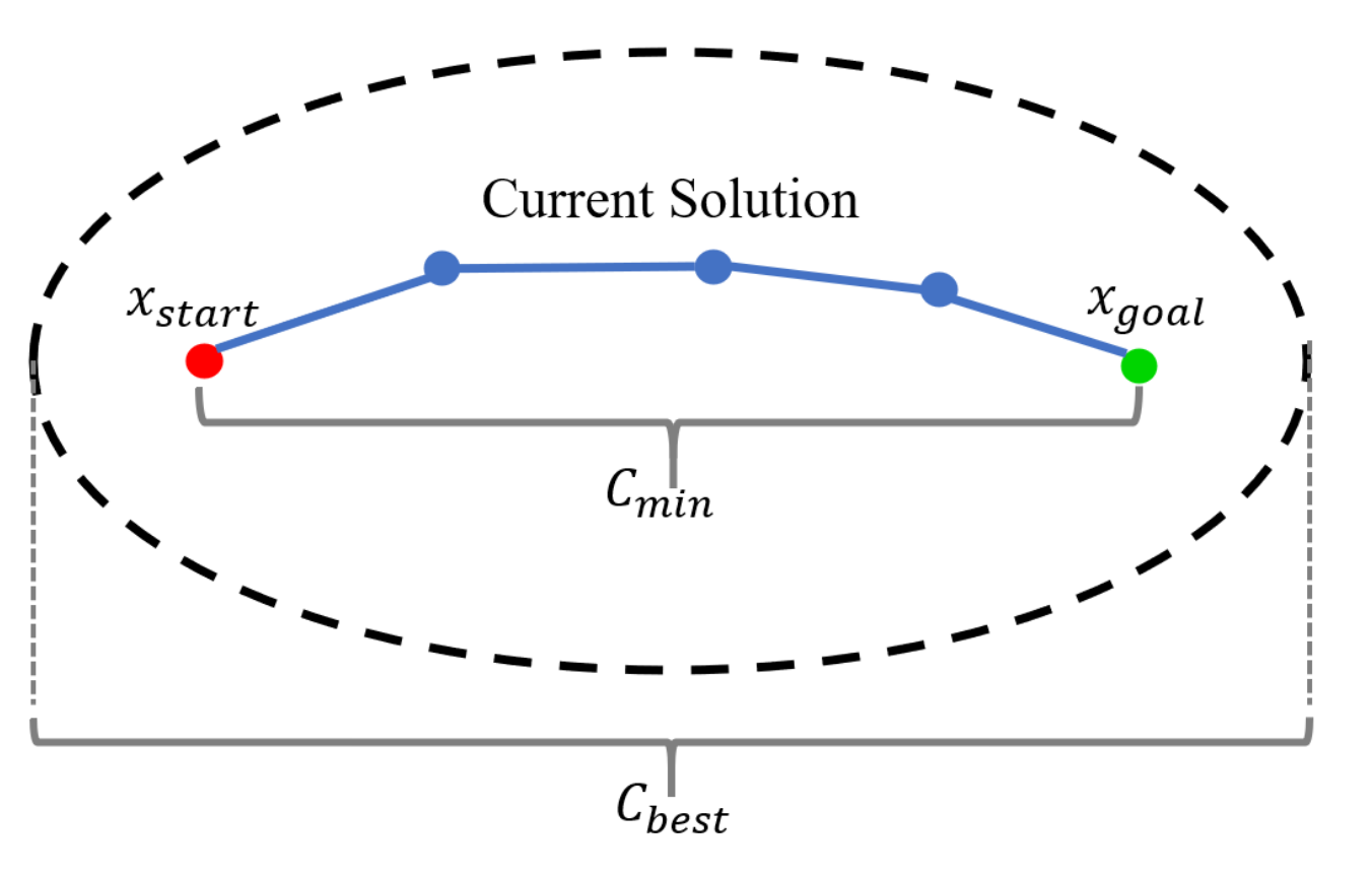
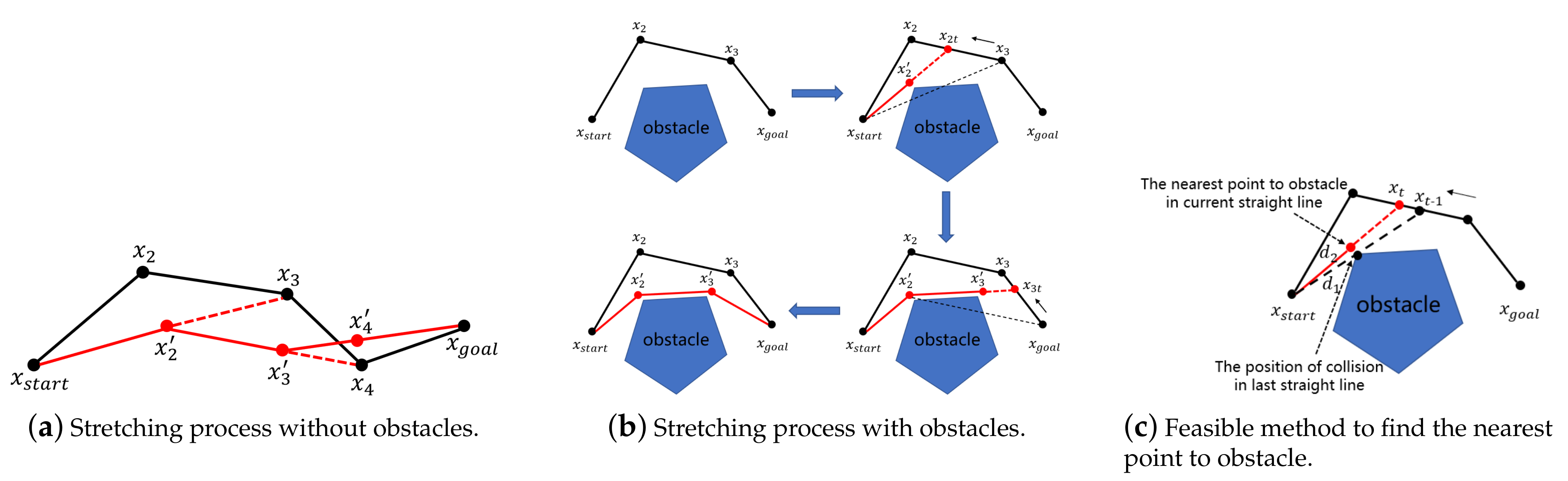
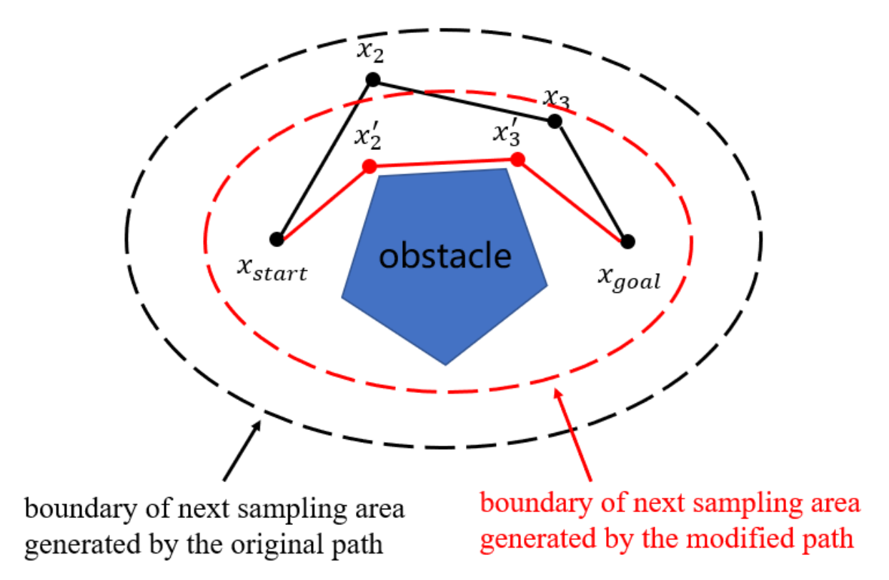
• During connecting the path points, the initial path may be tortuous so it always leads to unnecessary path cost. We adopt a simple stretch method to modify the connecting process and reduce the initial path cost. More importantly, the initial path cost determines the elliptical region in which samples in next iteration will improve the path. The modified BIT* with the stretch method can further reduce the size of elliptical region to accelerate the converging rate.
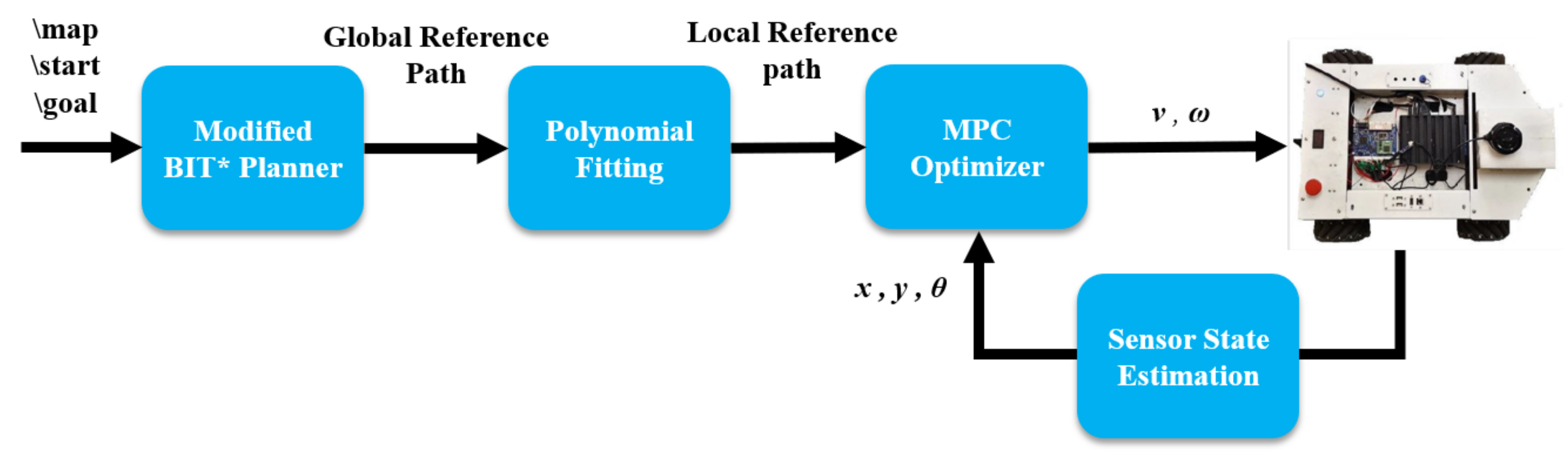
• After obtaining the global reference path with above method, we use the cubic polynomial curve to fit the reference path points in the robot coordinate system to obtain a local reference path which is smoother for a mobile robot to track.
• Then a nonlinear MPC method is adopted for trajectory tracking and speed generation considering obstacles near the robot.

A simplified illustration of the whole framework is shown in Figure 1.

The rest part of this paper is structured as below: In Section 2, three main parts of the proposed modified BIT* planner are introduced. The sample strategy of informed RRT* is introduced in Section 2.1. Section 2.2 shows the process of the stretch method. In Section 2.3, the modified BIT* algorithm is given. In Section 3, the MPC is implemented and the objective function is designed in Section 3.2. Section 4.2 compares the path found by three planners in two environments and demonstrates the better performance of proposed modified BIT*. The effectiveness of the whole framework is verified in Section 4.3. Finally, Section 5 makes a summary.

2. Modified BIT* Planner

In this section, in order to explain our stretch method and the modified BIT* planner, we firstly introduce the sampling strategy of basic informed RRT*. Then the second subsection explains the principle of this novel stretch method and how it can improve thee current path and accelerate the converging rate. The modified BIT* with the stretch method is also introduced in this section.

2.1. Sampling Strategy of Informed RRT*

In order to solve the sampling randomness of RRT* and improve converging rate. Informed RRT* is introduced in [14]. Firstly, it uses original RRT* to generate a initial path. After that, an ellipse with the start point and end point as the focal points and the path cost as the long axis is determined. For mobile robot’s path planning in 2-D space, we use X to represents the set of every point on the map. $g\left(x\right)$ and $h\left(x\right)$ denotes the cost from start state $x_{start}$ to a state $x\in X$ and the cost from x to goal state $x_{goal}$. For example, in Figure 2, we use Euclidean distance as cost function and $C_{best}$ denotes the length of current path solution ($C_{best}$ is infinity when there is no path solution). Then, an ellipse can be drawn. According to the properties of ellipse, we can get the following inequality:

$$\left|\right|x-x_{start}\left|\right|+\left|\right|x_{goal}-x\left|\right|<C_{best}$$

(1)

where x is inside this ellipse. Then we define the estimated cost $f\left(x\right)=g\left(x\right)+h\left(x\right)$. It is obvious that the estimated cost of x is less than current path cost $C_{best}$. So points within the ellipse have the potential to improve the current path solution.

In next iterations, the algorithm continue sampling to get a better solution. Rather than sampling in the whole map, the sampling point will be constrained in a unit circle and then they will be transformed to the ellipse area. The transformation process is illustrated in Algorithm 1 [14].

Matrix U and V is obtained by singular value decomposition of matrix M. The expression of M is shown as below:

$$\begin{array}{cc}\hfill & M=m{l}^T\hfill \\ \hfill & m=(x_{goal}-x_{start})/\left|\right|x_{goal}-x_{start}{\left|\right|}_2\hfill \end{array}$$

(2)

Algorithm 1:InformedSample($x_{start},x_{goal},C_{best}$).

2.2. Stretch Method

The process of stretch method is illustrated in Figure 3. Based on informed RRT*, we can obtain that the converging rate partially depends on the size of the ellipse area. In Figure 2, the current path is tortuous and it may lead to a large $C_{best}$. So we try to revise the current path to reduce it’s length. For the example in Figure 3, the black solid line is the original path. If there are no obstacles between the adjacent path points, we firstly connect $x_{start}$ and $x_3$, and then find the new next path point in the straight line. Actually, the new $x_2^{{}^{\prime }}$ only needs to be on the segment $x_{start}{x}_3$ to ensure that the new path is shorter than the original path. In order to roughly maintain the density of path points, we choose the position of $x_2^{{}^{\prime }}$ to make

$$\frac{x_{start}{x}_2^{{}^{\prime }}}{x_2^{{}^{\prime }}{x}_3}=\frac{x_{start}{x}_2}{x_2{x}_3}$$

(3)

and then we replace $x_2$ with new path point $x_2^{{}^{\prime }}$. Similarly, start from $x_2^{{}^{\prime }}$, the new path points $x_3^{{}^{\prime }}$, $x_4^{{}^{\prime }}$ satisfy $\frac{x_2^{{}^{\prime }}{x}_3^{{}^{\prime }}}{x_3^{{}^{\prime }}{x}_4}=\frac{x_2^{{}^{\prime }}{x}_3}{x_3{x}_4}$ and $\frac{x_3^{{}^{\prime }}{x}_4^{{}^{\prime }}}{x_4^{{}^{\prime }}{x}_{goal}}=\frac{x_3^{{}^{\prime }}{x}_4}{x_4{x}_{goal}}$. Finally, we connect $x_4^{{}^{\prime }}$ to the goal directly. The red solid line is the new path after the stretch method. Obviously, it is easy to prove that this new red path is shorter than the original one by using the principle that the sum of any two sides of a triangle is greater than the third side.

In most cases, there are obstacles in the environment, so we must consider this common situation. For example, in Figure 3b, the straight line between $x_{start}$ to $x_3$ will collide with the obstacles, so we find a point between $x_2$ and $x_3$ that could avoid collision when connecting with $x_{start}$. Then we select the point that is nearest to the obstacle as the next point and repeat this process until arriving to goal. In Figure 3a,b, the black line is the original path and the red line denotes the new path after stretching. We can obtain that the new path length is shorter that the original path. The new path length will be used as $C_{best}$ in the process of InformedSample shown in Algorithm 1. For example, in Figure 4, the black ellipse is the boundary of next sampling area generated by the original path according to the strategy of informed RRT*, and the red ellipse is the boundary generated by the modified path after stretch method. The sampling points in the red ellipse region are more likely to shorten the current path and speed up the convergence rate.

The complete algorithm is shown in Algorithm 2. This algorithm processes the stretch method through a loop until arriving to goal. P is the original path. ’NoCollision’ in line 5 is the process to check if there is obstacle between two path points. ’GetNext’ is to find a new path point to replace the original as is shown in Figure 3a, and the principle of selecting is described above. ’Divide’ in line 8 is to divide the line between two adjacent path point into several equal parts and then a series of path points are stored in a container (TemPoints in line 8). Next procedure is to find $x_t$ that can avoid collision among these path points. The black arrow in Figure 3b indicates the direction of the search. ’NeareatToObs’ is to get the nearest point to obstacle between $x_{current}$ and $x_t$.

In real implementation, it may be difficult to get the nearest point to obstacle from the information of grid map. There is a feasible method. For the example in Figure 3c. Firstly, we connect the $x_{current}$ and $x_{t-1}$ and then divide the straight line into a series path points. Next, we check these points one by one to see if they locate in collision area. Among the path points which are in collision area, we choose the point that nearest to $x_{t-1}$ as “The position of collision in last straight line” and calculate the distance from it to $x_{current}$ as $d_1$. Then, in current straight line between $x_{current}$ and $x_t$ that can avoid collision, we select the point that can satisfy $d_2=d_1$ as the nearest point to obstacle. Moreover, the obstacle cells in the map are enlarged by the robot radius r to keep the robot away from obstacles.

Algorithm 2:Stretch(P).

2.3. Modified BIT*

BIT* algorithm construct a tree that explores from start state to goal state. It maintains a vertex queue and an edge queue, then continuously select edges that have the potential to improve the current path from the edge queue [15]. We present a modified BIT* with the informed sample strategy as well as stretch method and the process of this modified BIT* is illustrated in Algorithm 3.

There are some notations used in the algorithm. The exploring tree consists of ‘Vertices’ and ‘Edges’. $g_{\tau }\left(v\right)$ is the cost from start to v through the current tree. ‘$c(v,x)$’ is the cost of an edge $(v,x)$. ‘$\widehat{h}\left(x\right)$’ is the heuristic function that guide the tree to explore towards the goal and we use the distance between x and goal to estimate it.

Many factors can be considered in path cost. In Section 2.2, the stretch method have been introduced to reduce the twists and turns of the path. And in our simulation, we use differential wheeled mobile robot to verify our modified BIT*. So we only consider the path length in $g_{\tau }\left(v\right)$ and we use the path length from start state to v to calculate it. Actually, for other robots which have steering angle limits, it is necessary to consider the curvature of the path in the cost function $g\left(x\right)$ and $c(v,x)$.

In Algorithm 3, ‘BestValueInVQ’ is to get the lowest estimated cost in ‘VetexQueue’ according to $g_{\tau }\left(x\right)+\widehat{h}\left(x\right)$, and ‘BestVertex’ return the vertex in ‘VertexQueue’ with lowest estimated cost. ‘BestValueInEQ’ is to get the lowest estimated cost in ‘EdgeQueue’ according to $g_{\tau }\left(v\right)+c(v,x)+\widehat{h}\left(x\right)$. Line 8 means that the best vertex has the potential to expand to get a better edge, so ‘Explore’ is to connect the best vertex and the near points in ‘Samples’ with radius r to get new edges, and then new edge $(v,x)$ that satisfy $g_{\tau }\left(v\right)+c(v,x)+\widehat{h}\left(x\right)<C_{best}$ is added to ‘EdgeQueue’. r can be defined as a variable and the specific expression is given in [15]. Then, the algorithm have to check if the best edge is able to improve the path (line 12). If the best edge can not improve the path, the current EdgeQueue and VertexQueue would be cleared and ‘Samples’ would be updated in next iteration. Algorithm 3 shows a simple description of our proposed modified BIT*.

Compared to original BIT*, we use a simple stretch method shown in Algorithm 2 when getting a new path, which is able to reduce the twists and turns as well as the path cost. The cost of stretched path will be used as $C_{best}$ to limit the sample area in next sampling process, accelerating the converging rate. In real implementation, the collision checking is necessary though it is not shown in Algorithm 3. Besides, the stretch method would be adopted only when a new path is found to reduce computational cost.

Algorithm 3:Modified BIT*.

3. MPC Method

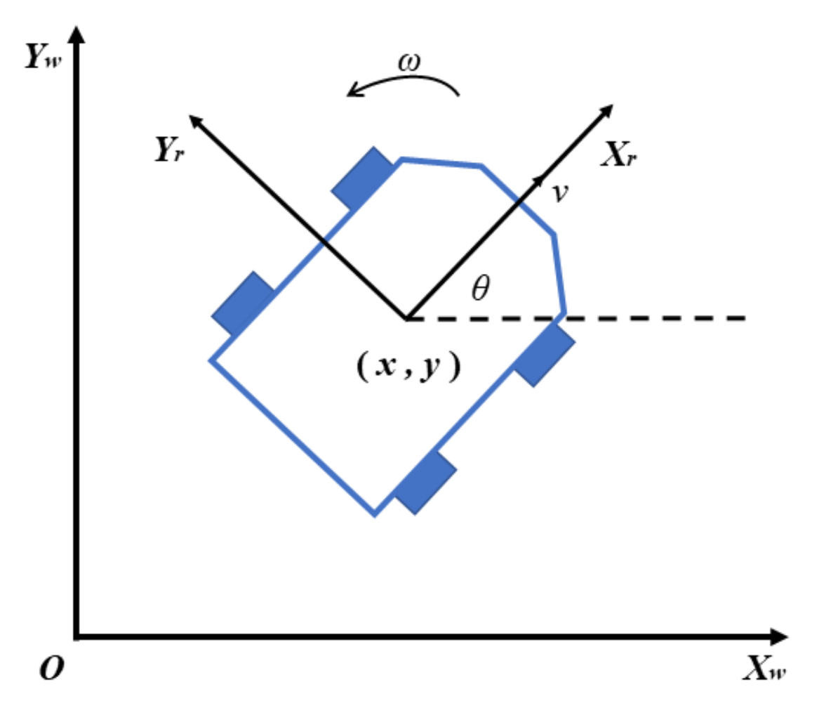
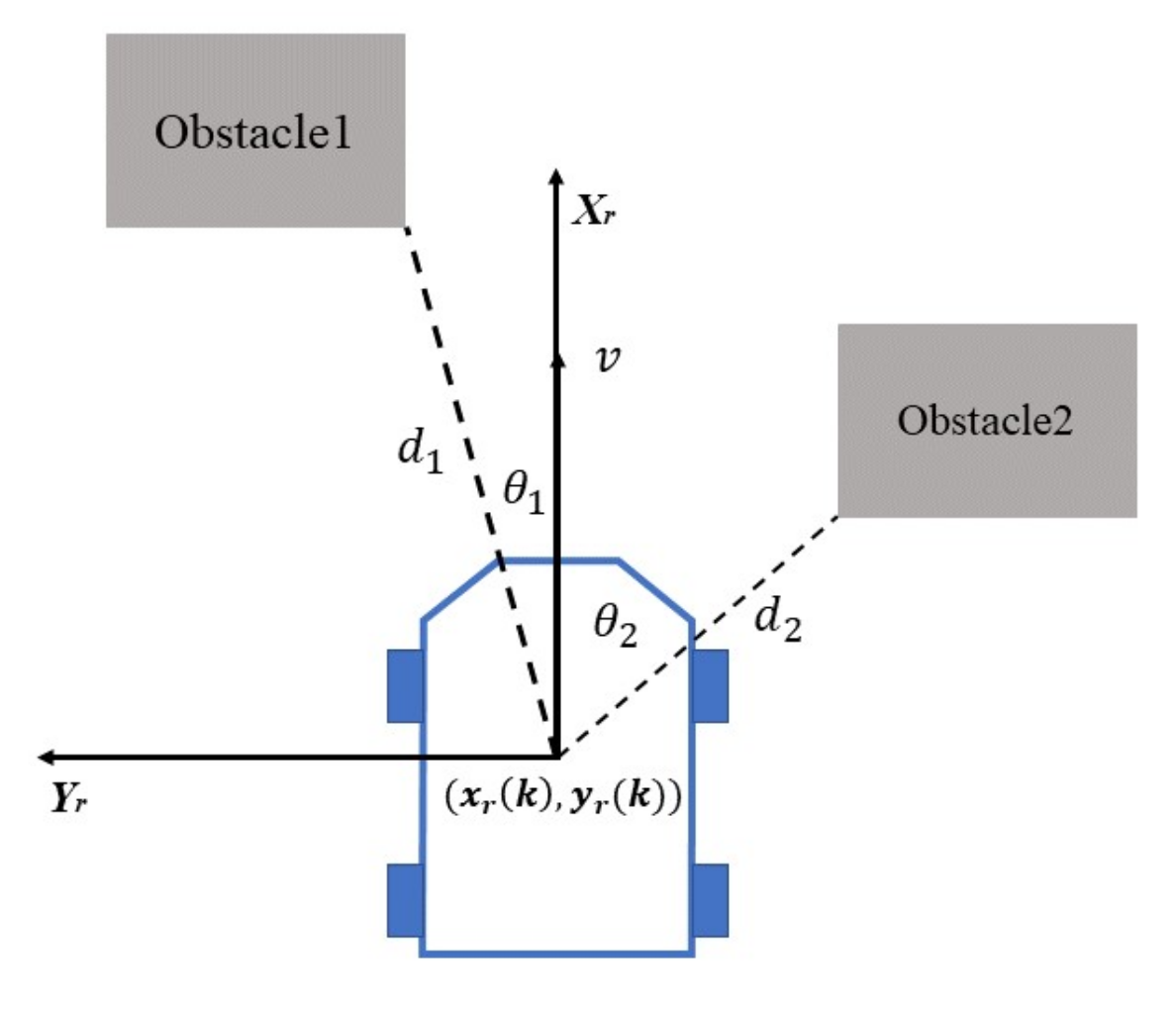
3.1. Kinematic Model

We select the kinematic model of a mobile robot as follows:

$$\left[\begin{array}{c}\dot{x}\\ \dot{y}\\ \dot{\theta }\end{array}\right]=R\left(\theta \right)\left[\begin{array}{c}{v}_x\\ v_y\\ \omega \end{array}\right]$$

(4)

where

$$R\left(\theta \right)=\left[\begin{array}{ccc}cos\theta & -sin\theta & 0\\ sin\theta & cos\theta & 0\\ 0& 0& 1\end{array}\right]$$

(5)

$(x,y)$ represents the position of the mobile robot in the world coordinate system and the $\theta$ denotes the yaw angle. $v_x$, $v_y$ represent the longitudinal velocity and lateral velocity respectively. Noticed that we set the lateral velocity $v_y$ to 0, and we use v in robot coordinate system to replace $v_x$. $\omega$ is the angular velocity of mobile robot. The two systems are shown in Figure 5.

After discretization of the above model, it can be obtained

$$\left[\begin{array}{c}x(k+i)\\ y(k+i)\\ \theta (k+i)\end{array}\right]=\left[\begin{array}{c}x(k+i-1)\\ y(k+i-1)\\ \theta (k+i-1)\end{array}\right]+\left[\begin{array}{cc}cos\theta (k+i-1)\Delta T& 0\\ sin\theta (k+i-1)\Delta T& 0\\ 0& \Delta T\end{array}\right]u(k+i-1)$$

(6)

$\Delta T$ is the sampling time. We use $u(k+i-1)={[v(k+i-1),\omega (k+i-1)]}^T$ to denote the control input at discrete time step $k+i-1$ [21].

3.2. Implementation of MPC

The global planner gets a series of path points. In order to make the trajectory of the robot more smoother and calculate the tracking error more conveniently, we can preprocess these path points. A feasible method is to fit the path points with the cubic polynomial curve. It should be noted that it is not necessary to fit all the path points, but to fit the path points within a certain distance in front of the robot, and then we can transform these reference path points to the robot coordinate system $X_r$–$Y_r$ which can be determined by the current state $(x_c,y_c,{\theta }_c)$—the current position and yaw angle in global coordinate system. For example, a reference path point $(x_g,y_g)$ in the global coordinate system can be transformed to $(x,y)$ in the robot coordinate system with following equations:

$$\begin{array}{cc}\hfill & x=(x_g-x_c)\ast \cos \left({\theta }_c\right)+(y_g-y_c)\ast \sin \left({\theta }_c\right)\hfill \\ \hfill & y=(y_g-y_c)\ast \cos \left({\theta }_c\right)-(x_g-x_c)\ast \sin \left({\theta }_c\right)\hfill \end{array}$$

(7)

Then, we use cubic polynomial curves to fit these path points after the transformation to the robot coordinate system

$$f\left(x\right)=m_0+m_{1}x+m_2{x}^2+m_3{x}^3$$

(8)

$m_0$, $m_1$, $m_2$ and $m_3$ are the coefficients of the polynomial, and they will be calculated online as the algorithm runs. In this way, we can use the analytic form of path $f\left(x\right)$ to easily calculate the tracking error and yaw error. An important task of MPC is to reduce tracking error. In Figure 6, the red dotted line denotes the local reference path $f\left(x\right)$. The tangent direction of $f\left(x\right)$ represents the desired yaw angle in $X_r$–$Y_r$. $(x_r\left(k\right)$, $y_r\left(k\right))$ is the initial position in $X_r$–$Y_r$, which is actually (0, 0). $x_r(k+i)$, $y_r(k+i)$ and ${\theta }_r(k+i)$ represent the predicted position and yaw angle respectively in $X_r$–$Y_r$ at time step $k+i$. As is shown in the figure, we can define the tracking error and yaw error at discrete time step $k+i$:

$$\begin{array}{cc}\hfill & e(k+i)=f\left(x_r(k+i)\right)-y_r(k+i)\hfill \\ \hfill & e_{\theta }(k+i)=arctan\left(f^{{}^{\prime }}\left(x_r(k+i)\right)\right)-{\theta }_r(k+i)\hfill \end{array}$$

(9)

Noticed that $arctan\left(f^{{}^{\prime }}\left(x_r(k+i)\right)\right)$, ${\theta }_r(k+i)$∈$[-\pi ,\pi ]$. The predicted state $(x_r(k+i),y_r(k+i),{\theta }_r(k+i))$ can be obtained through the kinematic Equation (6) ($i=1,2,3...N_p$).

The objective function is crucial for the performance of mobile robot. In our implementation, we choose the form of objective function as follows:

$$\begin{array}{cc}\hfill minJ=& \sum _{i=1}^{N_p}{a}_1{e}^2(k+i)+\sum _{i=1}^{N_p}{a}_2{e}_{\theta }^2(k+i)+\sum _{i=1}^{N_e}{\Delta u}^T(k+i)A_3\Delta u(k+i)\hfill \\ \hfill & +\sum _{i=1}^{N_e}{a}_4[\cos ({\theta }_1-\omega (k+i)\Delta T)/g\left(d_1\right)+\cos ({\theta }_2-\omega (k+i)\Delta T)/g\left(d_2\right)]\hfill \\ \hfill & +\sum _{i=1}^{N_p}{a}_5{(v(k+i)-v_d)}^2+\sum _{i=1}^{N_e}{a}_{6}v(k+i)/g\left(min(d_1,d_2)\right)\hfill \end{array}$$

(10)

$$\begin{array}{cc}\hfill s.t& 0\le v(k+i)\le v_{max}\hfill \\ \hfill & -{\omega }_{max}\le \omega (k+i)\le {\omega }_{max}\hfill \\ \hfill & -a_{max}\Delta T\le \Delta v(k+i)\le a_{max}\Delta T\hfill \\ \hfill & -{\alpha }_{max}\Delta T\le \Delta \omega (k+i)\le {\alpha }_{max}\Delta T\hfill \end{array}$$

(11)

In Equation (10), $N_p$ denotes the prediction horizon, and $N_e$ is the execute horizon. The first and second terms is to penalize the tracking error and yaw error. The robot should follow the reference trajectory generated by the global planner with small error, and the heading angle should fit the tangent direction of the trajectory. $a_1$ and $a_2$ are are two adjustable constant parameters.

In the third term of Equation (10), $\Delta u(k+i)$ represents the change of control input (linear velocity and angular velocity) at two adjacent moments and $\Delta u(k+i)=u(k+i)-u(k+i-1)$. The purpose of this term is to penalize the drastic variation of control input, so that the robot can move steady. $A_3$ is a $2\times 2$ constant diagonal matrix which can be set.

The fourth term is the repulsive function based on the direction of the obstacles. In our simulation, we do collision checking according to the cost map. Where there is an obstacle in the map, there will be a high “cost value”. The obstacle constraints cannot be expressed directly in analytic form, and it may be not convenient to add the obstacle constrains in the optimization. So we designed the repulsive function to penalize the linear velocity and angle velocity that make the robot move towards the obstacle. Actually, we only consider the nearest obstacles on the left and right sides in front of the robot. $g\left(d\right)$ is a function of the obstacle distance d, which is positively correlated with d. $d_1$ and $d_2$ represent the distances to the nearest obstacle on the left and right respectively. ${\theta }_1$ and ${\theta }_2$ denote the angle between the current velocity direction of the robot and the direction of the nearest obstacle on the left and right sides respectively. In our implementation, we choose the form of $g\left(d\right)$ as follows:

$$g\left(d\right)=\left\{\begin{array}{cc}p\ast d+q\hfill & d\le \mathrm{threshold}\hfill \\ \infty \hfill & d>\mathrm{threshold}\hfill \end{array}\right.$$

(12)

p and q are both positive constants. q is set so that $g\left(d\right)$ is always greater than 0 and it is set to a small value. The obstacles beyond the threshold can be ignored. In order to avoid collision with obstacles, the robot need to choose appropriate angular velocity to prevent it from being too close to the obstacles. For example, in Figure 7, suppose the robot is more affected by the repulsive function of the obstacle on the left side, the angular velocity that makes the robot approach the left obstacle will be more penalized by the repulsive function. So the angular velocity is set to negative, making the robot turn right to avoid getting close to the obstacle.

The last two terms of Equation (10) is to make the robot maintain a desired stable speed during the movement and slow down when approaching obstacles. The desired speed $v_d$ can be set to a value smaller than the maximum speed of the robot according to different requirements. In addition, the robot needs to slow down according to the distance from the nearest obstacle. In summary, the parameters $a_1$, $a_2$, $A_3$, $a_4$, $a_5$ and $a_6$ in objective function determine different optimization objectives. For instance, when $a_1$ and $a_2$ are increased, the robot tends to follow the reference path. When $a_4$ is increased, the robot is more likely to respond to the nearby obstacles, resulting in the actual path deviates from the reference path.

Equation (11) are the constrains of the optimization problem. $v_{max}$ and ${\omega }_{max}$ are the maximum linear velocity and maximum angular velocity of the mobile robot respectively. $a_{max}$ and ${\alpha }_{max}$ are the maximum linear and angular acceleration respectively. These constraints are determined by the robot hardware and cannot be violated.With objective function (10) and constraints Equation (11), the optimal control inputs can be calculated by solving the nonlinear programming problem.

In our work, we design the controller based on kinematics in ROS, and then send the linear velocity and angular velocity to the bottom controller of the robot in the simulation platform. The bottom controller based on the dynamics of the robot has been designed so we do not care about it here.

4. Simulation

4.1. Simulation Setting

In order to show the performance of our proposed method, we implemented RRT*, BIT* and modified BIT* in ROS (robot operating system) and use them as global planner to generate reference path. The map is generated through gmapping in ROS and the resolution is 0.05 m. Where there is an obstacle in the map, there will be a high “cost value”. So we can do collision checking according to the cost map. The environment and paths are displayed in rviz, which is a popular visualization tool in ROS. In this section, firstly we use RRT*, BIT* and the proposed modified BIT* to generate reference global path. In this paper, we take the path length as the path cost, and we compare the path length, the iterations and computational time in difference algorithm to verify the better performance of the modified BIT*, as the less iterations means faster converging rate.

Then, we use the modified BIT* to obtain reference path. MPC method is applied for trajectory tracking and motion control, and the performance of our proposed framework will be illustrated in different scenario.

4.2. Modified BIT* Planner

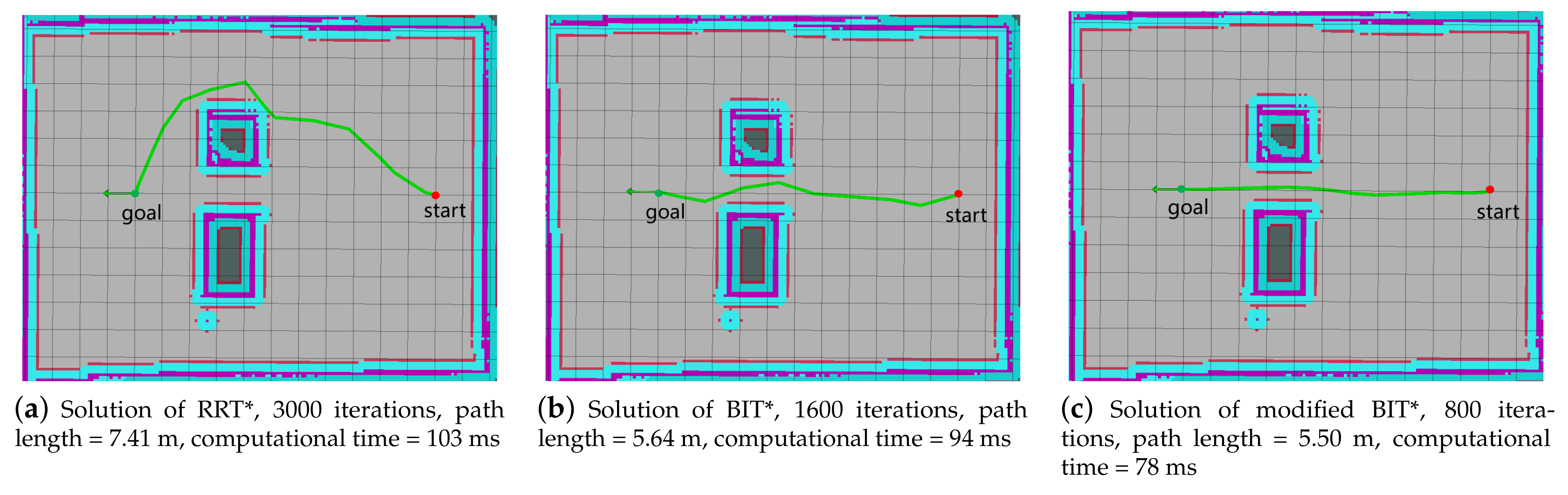
• Few obstacles with narrow channel: Figure 8 shows the environment with fewer obstacles and a narrow channel. The coordinates of the start point and the goal point are (0 m, 0 m) and (0 m, 5.5 m) respectively. The green solid line is the path generated by the global planner. From the map, we can see that there are two obstacle between start and goal, and the optimal path for mobile robot is to across the narrow channel between the obstacle. For sampling-based planning algorithm that uses a random sampling method like RRT*, the sampling points are rarely located in the narrow channel. So it is difficult to find an good path when iterations are not enough. In Figure 8a, instead of passing through a narrow channel, the path found by RRT* after 3000 iterations bypasses the obstacles above to the goal. In addition, this path has unnecessary twists and turns, which is not suitable for mobile robots. Figure 8b shows the solution of BIT*. Compared with RRT*, BIT* successfully found a path through the narrow channel and it uses 1600 iterations. However, in our multiple tests, BIT* does not always find a solution as shown in Figure 8b and sometimes BIT* can only find a path around obstacles with 1600 iterations. The path from start to goal in Figure 8c shows the better performance of our proposed method. Benefit from the stretch method, the modified BIT* can find a shorter and smoother path through the narrow channel with less iterations.
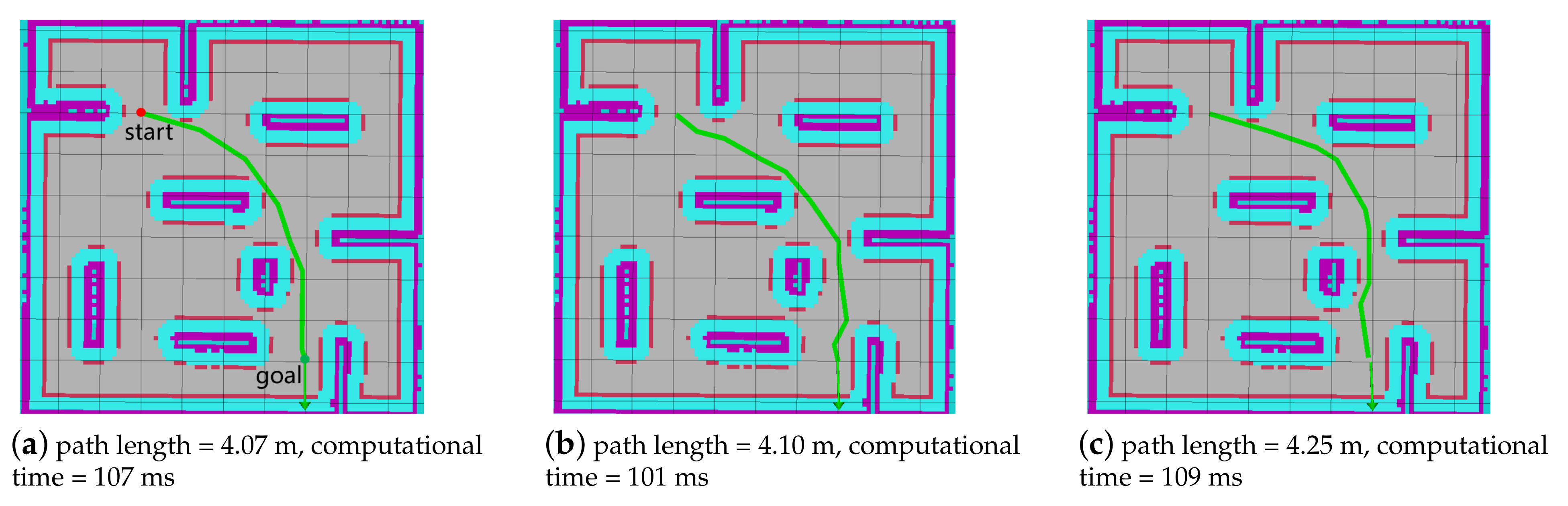
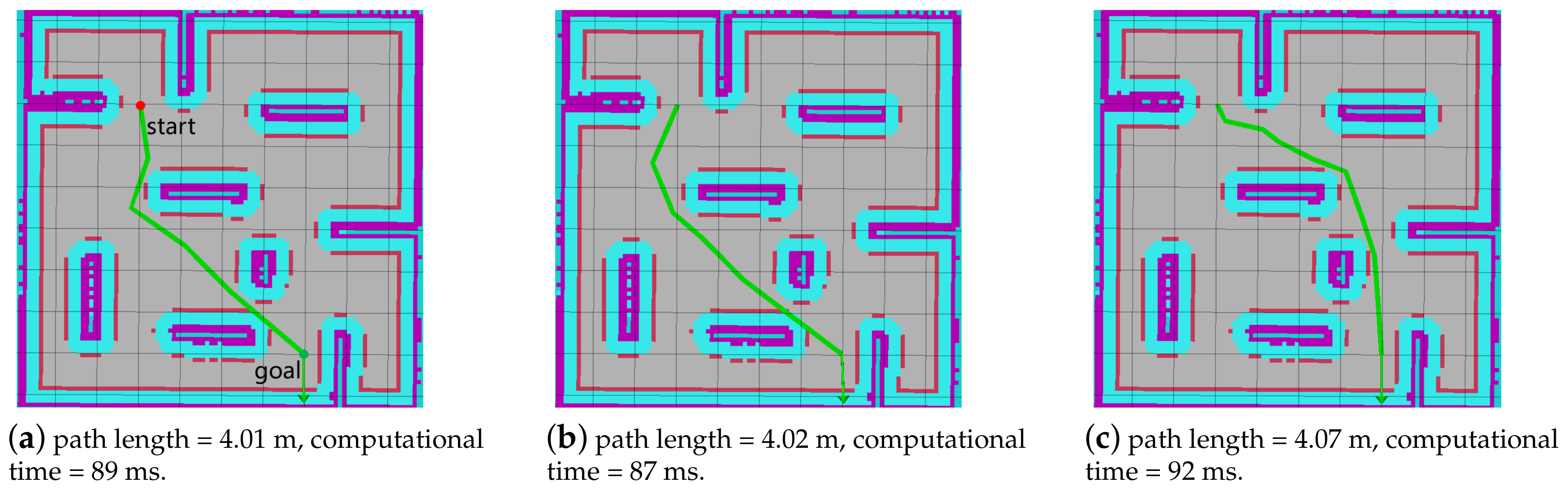
• Multiple obstacles: In practical applications, mobile robots may need to plan a collision-free path in environment with multiple obstacles. Based on this requirement, we design an environment shown in Figure 9, Figure 10 and Figure 11 with intensive obstacles to test the performance of the three planners. The coordinates of the start point and the goal point are (0 m, 0 m) and (−3 m, −2 m) respectively. Firstly, by observing the map, we can know that there are two kinds of good paths from the start to goal. One is to across the top left of goal, the other is through the top of the goal. So we show three different solutions for each planner to see that which kind of solutions these planners tend to select.

In Figure 9, the paths found by RRT* with 3000 iterations are through top of the goal. However, the cost of these paths always are higher than those generated by the other two planners. Besides, some unnecessary turns occur in the path, resulting in relatively high cost, as shown in Figure 9b,c. In Figure 10, with 1600 iterations, BIT* tend to find paths through the top left of the goal in most cases, which is shorter than paths found by RRT*. Modified BIT* can always find shorter path that is through the top left of the goal only with 800 iterations, much less than BIT* and RRT*, as shown in Figure 11. Compared to above two planners, the path found by modified BIT* is much smoother that is more suitable for mobile robot.

Table 1. The average of ten results of three planners.

Planner	Path Length (m)	Iterations	Computational Time (ms)
RRT*	4.16	3000	106.3
BIT*	4.05	1600	90.6
Modified BIT*	3.92	800	64.2

shows the average of the 10 planning results of the three planners in this scenario.

Due to the simple stretch method, no matter in the environment with few obstacles or dense obstacles, our proposed modified BIT* always find shorter path than BIT* and RRT* with less iterations which is meaning faster converging rate.

4.3. Whole Framework

In this section, we use the model of Turtlebot robot in ROS to verify the effectiveness of our proposed framework. Firstly modified BIT* planner explores a reference path according to the preset starting point and goal point. Then the MPC method proposed in Section 3.2 calculates the optimal control inputs (linear velocity and angular velocity) and send them to the robot. Some necessary parameter settings are in

Table 2. Parameters in MPC method.

Prameters	Value	Parameters	Value	Parameters	Value
$\Delta T$	0.1 (s)	$A_3$	diag{50, 20}	p	10
$N_p$	20	$a_4$	40	q	0.05
$N_e$	2	$a_5$	30	threshold	0.8 (m)
$a_1$	60	$a_6$	2	$v_{max}$	0.5 (m/s)
$a_2$	50	$v_d$	0.3 (m/s)	${\omega }_{max}$	0.6 (rad/s)

.

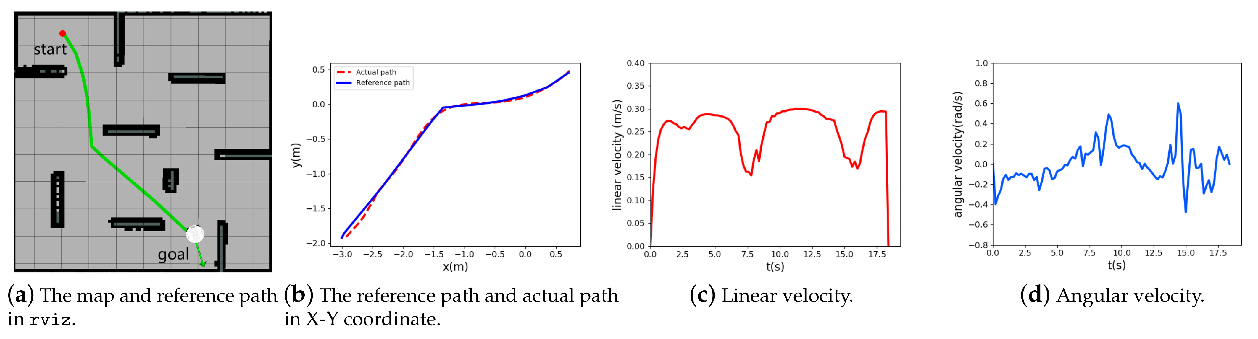
• Few obstacles with narrow channel: Figure 12a shows the map and the reference path generated by modified BIT* planner. The reference path and actual path of mobile robot are illustrated in Figure 12b. The coordinates of the start point and the goal point are (1 m, 1 m) and (0 m, 5.5 m) respectively. Actually, the actual path does not track the reference path perfectly. Because the repulsive function is added into the objective function of MPC method, the actual path deviates from the reference path in the place close to the obstacle, so that the robot will not be too close to the obstacle to avoid possible collision. Moreover, the ratio of parameters $a_1$, $a_2$ and $a_4$ is also an important factor, and the robot may tend to stay away from the obstacles rather than track the reference trajectory in this situation. So we can adjust the ratio of $a_1$, $a_2$ and $a_4$ to make the robot behave differently. Figure 12c,d show the variation of linear velocity and angular velocity with time respectively. During 6s to 8s, the robot approaches the obstacle, and according to the design of the objective function, the robot will decelerate appropriately. At the same time, the angular velocity will be adjusted according to the position of the obstacle, resulting in fluctuation. Most of the time, the robot will move at the desired speed (0.3 m/s).
• Multiple obstacles: Figure 13a shows an environment with many obstacles and the reference path. Mobile robot need to react to these obstacles in time when it moves along the reference path. In Figure 13b, the blue solid line represents the reference path, and the red dotted line represents the actual path of the robot. The coordinates of the start point and the goal point are (0.7 m, 0.45 m) and (−3 m, −1.95 m) respectively. Similar to the previous case, the actual path does not exactly coincide with the reference path. There is slight deviation in the three sections near the obstacle to ensure safety. In Figure 13c, due to its proximity to the obstacle, the robot slows down during 1 s–2.5 s, 6 s–7.5 s and 13 s–15 s, which shows that the robot can decelerate in time when approaching multiple obstacles. As the robot approaches the obstacle and decelerates, the angular velocity of the robot will fluctuate, so as to adjust the direction of movement and keep away from the obstacle, which can be seen in Figure 13d.

The performance in these two case shows the effectiveness of the proposed methods. On the one hand, the mobile robot can find shorter path with less time. On the other hand, the robot is able to react to the obstacles in time to avoid possible collision, as well as track the reference path.

5. Conclusions

In this paper, for motion planning of mobile robot, we firstly proposed a modified BIT* with a stretch method. The stretch method can further reduce the size of the sampling area when BIT* find a new path, and each sample point in this area have the potential to improve the current path, so it can find better solution with less iterations and computational time. Besides, the stretch method can also avoid some unnecessary turns in the path. With this method, a reference path suitable for mobile robot can be obtained. Next, we use MPC method for trajectory tracking and motion control. Even though the obstacles in the map are enlarged, the repulsive function in the MPC method based on the distance and direction of obstacles is added to the objective function to avoid being to close to obstacles and ensure safety. Finally, we compare the performance of RRT*, BIT* and the modified BIT* in two different environment and the results show that the proposed modified BIT* can find better path with faster converging rate. The effectiveness of the whole framework is also verified both in the environment with few obstacles and multiple obstacles. The results show that the actual trajectory may deviate from the reference trajectory due to the repulsive function, but parameters could be adjusted to balance the tracking performance and the tendency to keep away from obstacle. In future work, we plan to verify and test our method on a real robot platform, and improve and upgrade our method for different robots. Furthermore, we will consider the dynamics of mobile robot in our controller design.

References

1. Khatib, O. Real-time obstacle avoidance for manipulators and mobile robots. In Proceedings of the 1985 IEEE International Conference on Robotics and Automation, St. Louis, MO, USA, 25–28 March 1985; Volume 2, pp. 500–505. [Google Scholar]
2. Dijkstra, E.W. A Note on Two Probles in Connexion with Graphs. Numer. Math. 1959, 1, 269–271. [Google Scholar] [CrossRef] [Green Version]
3. Hart, P.E.; Nilsson, N.J.; Raphael, B. A Formal Basis for the Heuristic Determination of Minimum Cost Paths. IEEE Trans. Syst. Sci. Cybern. 1968, 4, 100–107. [Google Scholar] [CrossRef]
4. Kavraki, L.E.; Svestka, P.; Latombe, J.; Overmars, M.H. Probabilistic roadmaps for path planning in high-dimensional configuration spaces. IEEE Trans. Robot. Autom. 1996, 12, 566–580. [Google Scholar] [CrossRef] [Green Version]
5. LaValle, S.M.; Kuffner, J.J. Randomized kinodynamic planning. In Proceedings of the 1999 IEEE International Conference on Robotics and Automation (Cat. No.99CH36288C), Detroit, MI, USA, 10–15 May 1999; Volume 1, pp. 473–479. [Google Scholar]
6. Urmson, C.; Simmons, R. Approaches for heuristically biasing RRT growth. In Proceedings of the 2003 IEEE/RSJ International Conference on Intelligent Robots and Systems (IROS 2003) (Cat. No.03CH37453), Las Vegas, NV, USA, 27–31 October 2003; Volume 2, pp. 1178–1183. [Google Scholar]
7. Kuffner, J.J.; LaValle, S.M. RRT-connect: An efficient approach to single-query path planning. In Proceedings of the 2000 ICRA. Millennium Conference, IEEE International Conference on Robotics and Automation, Symposia Proceedings (Cat. No.00CH37065), San Francisco, CA, USA, 24–28 April 2000; Volume 2, pp. 995–1001. [Google Scholar]
8. Karaman, S.; Frazzoli, E. Sampling-Based Algorithms for Optimal Motion Planning. Int. J. Robot. Res. 2011, 30, 846–894. [Google Scholar] [CrossRef]
9. Karaman, S.; Frazzoli, E. Optimal kinodynamic motion planning using incremental sampling-based methods. In Proceedings of the 49th IEEE Conference on Decision and Control (CDC), Atlanta, GA, USA, 15–17 December 2010; pp. 7681–7687. [Google Scholar]
10. Hasan, O. RRT*-Smart: Rapid convergence implementation of RRT* towards optimal solution. In Proceedings of the International Conference on Mechatronics & Automation, Chengdu, China, 5–8 August 2012. [Google Scholar]
11. Dillmann, R. RRT*-Connect: Faster, Asymptotically Optimal Motion Planning. In Proceedings of the 2015 IEEE International Conference on Robotics and Biomimetics (ROBIO 2015), Zhuhai, China, 6–9 December 2015. [Google Scholar]
12. Persson, S.M.; Sharf, I. Sampling-Based A * Algorithm for Robot Path-Planning. Int. J. Robot. Res. 2014, 33, 1683–1708. [Google Scholar] [CrossRef]
13. Pavone, M. Fast Marching Tree: A Fast Marching Sampling-Based Method for Optimal Motion Planning in Many Dimensions. Int. J. Robot. Res. 2015, 34, 883–921. [Google Scholar]
14. Gammell, J.D.; Srinivasa, S.S.; Barfoot, T.D. Informed RRT*: Optimal sampling-based path planning focused via direct sampling of an admissible ellipsoidal heuristic. In Proceedings of the 2014 IEEE/RSJ International Conference on Intelligent Robots and Systems, Chicago, IL, USA, 14–18 September 2014; pp. 2997–3004. [Google Scholar]
15. Gammell, J.D.; Srinivasa, S.S.; Barfoot, T.D. Batch Informed Trees (BIT*): Sampling-based optimal planning via the heuristically guided search of implicit random geometric graphs. In Proceedings of the 2015 IEEE International Conference on Robotics and Automation (ICRA), Seattle, WA, USA, 26–30 May 2015; pp. 3067–3074. [Google Scholar]
16. Huynh, H.N.; Verlinden, O.; Vande Wouwer, A. Comparative Application of Model Predictive Control Strategies to a Wheeled Mobile Robot. J. Intell. Robot. Syst. 2017, 87, 81–95. [Google Scholar] [CrossRef]
17. Li, W.; Yang, C.; Jiang, Y.; Liu, X.; Su, C.Y. Motion Planning for Omnidirectional Wheeled Mobile Robot by Potential Field Method. J. Adv. Transp. 2017, 2017, 4961383. [Google Scholar] [CrossRef]
18. Kong, H.; Yang, C.; Li, G.; Dai, S.L. A sEMG-Based Shared Control System with No-Target Obstacle Avoidance for Omnidirectional Mobile Robots. IEEE Access 2020, 8, 26030–26040. [Google Scholar] [CrossRef]
19. Chen, W.; Wang, N.; Liu, X.; Yang, C. VFH* Based Local Path Planning for Mobile Robot. In Proceedings of the 2019 2nd China Symposium on Cognitive Computing and Hybrid Intelligence (CCHI), Xi’an, China, 21–22 September 2019; pp. 18–23. [Google Scholar]
20. Teatro, T.A.V.; Eklund, J.M. Nonlinear model predictive control for omnidirectional robot motion planning and tracking. In Proceedings of the 26th IEEE Canadian Conference on Electrical and Computer Engineering (CCECE), Regina, SK, Canada, 5–8 May 2013; pp. 1–4. [Google Scholar]
21. Liu, J.; Jayakumar, P.; Stein, J.L.; Ersal, T. Combined Speed and Steering Control in High-Speed Autonomous Ground Vehicles for Obstacle Avoidance Using Model Predictive Control. IEEE Trans. Veh. Technol. 2017, 66, 8746–8763. [Google Scholar] [CrossRef]
Figure 1. The whole framework: Firstly the modified BIT* (batch informed trees) planner get a path according start state, goal state and the map. Then the MPC (Model Predictive Control) optimizer find the optimal control sequence v and ω and send them to the mobile robot as motion command.
Applsci 11 00426 g001
Figure 2. Informed RRT* (rapidly-exploring random tree): Once a path is generated, an ellipse is determined by the start state, goal state and path cost.
Applsci 11 00426 g002
Figure 3. The process of stretching method in different situation.
Applsci 11 00426 g003
Figure 4. The boundary of sampling area determined by the modified path after stretch method.
Applsci 11 00426 g004
Figure 5. The coordinate system of a mobile robot.
Applsci 11 00426 g005
Figure 6. The definition of tracking error and yaw error.
Applsci 11 00426 g006
Figure 7. The situation with obstacles.
Applsci 11 00426 g007
Figure 8. The performance of three planner in a scenario with few obstacles and a narrow channel.
Applsci 11 00426 g008
Figure 9. Solutions of RRT* in a scenario with multiple obstacles, 3000 iterations.
Applsci 11 00426 g009
Figure 10. Solutions of BIT* in a scenario with multiple obstacles, 1600 iterations.
Applsci 11 00426 g010
Figure 11. Solutions of modified BIT* in a scenario with multiple obstacles, 800 iterations.
Applsci 11 00426 g011
Figure 12. The performance of the whole framework in a scenario with few obstacles and a narrow channel.
Applsci 11 00426 g012
Figure 13. The performance of the whole framework in a scenario with multiple obstacles.
Applsci 11 00426 g013