Abstract
Flatbed scanners (FBSs) provide non-contact scanning capabilities that could be used for the on-machine verification of layer contours in additive manufacturing (AM) processes. Layer-wise contour deviation assessment could be critical for dimensional and geometrical quality improvement of AM parts, because it would allow for close-loop error compensation strategies. Nevertheless, contour characterisation feasibility faces many challenges, such as image distortion compensation or edge detection quality. The present work evaluates the influence of image processing and layer-to-background contrast characteristics upon contour reconstruction quality, under a metrological perspective. Considered factors include noise filtering, edge detection algorithms, and threshold levels, whereas the distance between the target layer and the background is used to generate different contrast scenarios. Completeness of contour reconstruction is evaluated by means of a coverage factor, whereas its accuracy is determined by comparison with a reference contour digitised in a coordinate measuring machine. Results show that a reliable contour characterisation can be achieved by means of a precise adjustment of image processing parameters under low layer-to-background contrast variability. Conversely, under anisotropic contrast conditions, the quality of contour reconstruction severely drops, and the compromise between coverage and accuracy becomes unbalanced. These findings indicate that FBS-based characterisation of AM layers will demand developing strategies that minimise the influence of anisotropy in layer-to-background contrast.
1. Introduction
Additive manufacturing (AM) processes have reached a high degree of maturity during the last decade. Evolving from a reduced number of applications, mainly related to aesthetic models and conceptual prototypes, AM is currently formed by a growing number of processes capable of achieving small-to-medium batch size productions and industrial-level requirements. This evolution has been sustained on better machines and processes capable of handling diverse materials, but also on reducing the gap between AM parts’ quality and that achieved with traditional manufacturing processes. In any case, according to Gartner, complete industrial adoption of AM is still 5 to 10 years away [1]. There are many reasons behind this gap in development, but a frequently highlighted issue is the difference between dimensional and geometrical accuracy achieved in AM parts, when compared with traditional manufacturing [2]. The usual approach regarding dimensional or geometrical assessment of AM parts is to measure or verify the final 3D part, once it has already been released from the machine [3,4]. Nevertheless, a tendency involving on-machine measurement (OMM) approaches with integrated measuring devices is currently gaining momentum [5,6,7,8]. These approaches will provide clear advantages when they become fully developed and incorporated to production-level machines [9]. Hence, dimensional inaccuracies would be detected when the part is still being manufactured, allowing the system to apply corrective actions or to stop production. In both cases, savings in terms of cost and time or related to non-conformities would be obtained.
Among the technologies that could be incorporated to production machines for quality verification, those not requiring contact between sensor and material, such as image sensors, triangulation lasers, or structured light, have several advantages. Non-contact technologies have nearly no influence upon parts, and are also faster than contact ones. Nevertheless, they are also usually worse in terms of accuracy. Flatbed scanners (FBSs) are optical devices that can be used for digitising flat objects. Although they are usually employed to scan paper sheets or photographs, computer vision techniques also enable them to be used in complex tasks. Among those tasks, several researchers have highlighted the use of FBSs for detecting contours of three-dimensional objects [10,11] and characterising surface defects [7]. This latter work illustrates the possibilities of using FBSs for on-machine verification and closed-loop manufacturing strategies.
Contour measurement with FBSs is severely affected by image deformation, which is a common issue to other image capturing devices. Some researchers have related image deformation in FBSs to mechanical errors of the equipment [12]. Accordingly, some works have focused on the possibilities of modelling and adjusting errors to improve measurement reliability [13,14]. Other works have pointed out the relevance of the relative position of the object with respect to the scanner plate or even the resolution, but also indicate that objects could be measured with sufficient accuracy if the sources of measurement variation were quantified and minimised [15].
The works by De Vicente [16] and Majarena [17] have provided a method for adjusting global deformation errors in FBS. Their approach improved the reliability of digital image-based analysis of part contours to a point that even manufacturing errors can be characterised and partially compensated. Blanco [18] proposed an alternative method for deformation adjustment and compensation, based on local deformation adjustment (LDA). Results upon a highly contrasted test specimen showed that, under specific test conditions, the characterisation of layer contours with a FBS could approximate the performance of a coordinate measurement machine (CMM).
Although some efforts were mainly oriented to adjust image distortion, a feasible characterisation of contours is also affected by additional sources of error. Solomon [19] mentions three factors that are key to contour detection: context, noise, and location. Context refers to the significance of the change in local intensity that indicates that a certain point is part of an edge, and relates this significance to that observed in the neighbourhood. In the case of AM layer contour characterisation, layer-to-background contrast shall be the main factor affecting context. Noise refers to the possibility of misidentifying noisy points as edge points. Accordingly, noise filtering shall be considered as a possible factor influencing contour characterisation. Location refers to the fact that the digital image of an edge reflects a smooth transition between intensity levels, which makes it difficult to fix with high accuracy which point represents the exact location of such transition. This factor shall be affected by the image processing sequence, especially by the method or algorithm used to distinguish between contour and its neighbourhood (edge detector). It shall also be affected by the actual value of the parameter used to make this distinction. According to Jain [20], an edge detector is “an algorithm that produces a set of edges from an image”, while a contour would be a “list of edges” or “the mathematical curve that models a list of edges”.
Previous research has not paid much attention to the influence of the image processing sequence and its specific configuration in the accuracy of the results. In most cases [10,11,16,18], both filtering and edge detection stages as well as their correspondent configurations are directly given, and no discussion about their possible influence on the results is provided. Even more, some works rely on manual measurement of the characteristics in the image, so they did not really use image processing or automatic contour detection algorithms [12,13,14,15,17]. Nevertheless, edge detection is a relevant part of every automated measurement strategy, and the effect of image processing configuration should not be neglected.
In their review of contour detection methods, Papari et al. [21] distinguished between region-oriented approaches, edge-and-line oriented approaches, and hybrid approaches. Other authors [22] include other categories, such as deep learning-based approaches. In the present research, analysis was limited to local edge detection methods that use differential operators [21] to search in a digital image for significant changes in local intensity with the objective of extracting a list of possible locations (i,j) of edge points. According to Spontón [23], two main approaches to edge detection based on differential operators are commonly used: first derivative approaches and second derivative approaches.
First derivative detectors seek for significant changes in a continuous function of image intensity by means of computing a gradient operator (∇) that is defined as a vector (Equation (1)).
This vector reflects the magnitude of the gradient at a given point G(x,y) and its angle with respect to the coordinate system of reference Ѳ(x,y). Nevertheless, a digital image does not really contain continuous functions of intensity. Instead, it is formed by arrays of discrete samples of ideally continuous functions. Consequently, so-called first derivative edge detectors approximate continuous functions by discrete ones. There are three main edge detectors based on the first derivative approach as proposed by Roberts [24], Sobel [25] and Prewitt [26]. These methods provide a new image of identical size as the original one, with each pixel representing the value of the gradient in its exact position on the original image. These operators use two kernels which are convolved with the original image to calculate approximations of the derivatives, in two perpendicular directions. Each method employs different kernels: Roberts´ kernel is intended for edges at 45°, whereas Prewitt and Sobel respond better to horizontal and vertical edges (Equation (2)).
Once the gradient for each direction is calculated (vertical and horizontal direction), a general magnitude (Equation (3)) and direction (Equation (4)) can be calculated:
A new grey scale image is obtained, with each grey value representing the gradient magnitude |G| calculated for the corresponding pixel on the original image. In these methods, any pixel of the new image will be considered a boundary if the value of its gradient |G| is higher than a threshold T. It should be noted that the Prewitt operator is expected to provide noisier results, because it uses a simpler approximation matrix than the Sobel technique [27].
Second derivative detectors, on the other hand, are based on the fact that a peak or valley on the first derivative would appear as a zero-crossing in the second derivative. One of these methods is based on the Laplacian calculation of the original greyscale image. An approximation of the second derivative can be calculated by means of a discrete convolution kernel, that can include diagonals or not (Equation (5)).
Using one of these kernels, the Laplacian can be calculated using standard convolution methods. These kernels are approximating a second derivative measurement on the image; therefore, they are very sensitive to noise. Due to this approach also being isotropic, no information about edge orientation is obtained. Another possible second derivative method uses the Laplacian of Gaussian (LoG) kernel, that can be calculated in advance, so that only one convolution needs to be performed at run-time on the image. The 2-D LoG function centred on zero, with Gaussian standard deviation σ, can be expressed as:
Note that as the Gaussian is made increasingly narrow, the LoG kernel becomes the same as the simple Laplacian kernels. The smoothing level is controlled by means of the standard deviation σ. In a subsequent step, zero-crossing must be found for each row and column.
The Canny method has also been considered in this study because, according to Papari [21], it is by far the most used differential operator. Canny is actually a multi-step algorithm that computes the gradient using Sobel or a derivative Gaussian filter. The steps that compose this method are reflected in Figure 1.
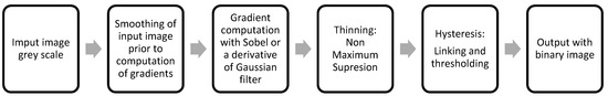
Figure 1.
Processing steps of Canny edge-detection method.
The first step involves applying a Gaussian filter to smooth the image to remove the noise. The next step is used to calculate the intensity gradients. The original formulation of this method used the Sobel kernel, whereas alternative formulations employ a derivative Gaussian filter. The result of this stage is a new image with wider edges; thus, a thinning stage by means of a non-maximum suppression technique is applied. The Canny method employs a double threshold to classify the pixels of the edges: strong edges are those pixels whose intensity is higher than the higher threshold, whereas weak edges are those between lower and higher thresholds. Pixels that present gradient values below the lower threshold are eliminated. Weak edges that are not connected with a strong edge are also eliminated from the final binary image.
Summarising, a reliable characterisation of AM layer contours should include geometrical information that enables the description and measurement of discrepancies between actual (manufactured) contours and their theoretical definition. Digital images of each layer provided by an FBS shall be processed considering the noise filtering, the edge-detection method and the criterion used to promote edge candidates to contour points. Additionally, the layer-to-background contrast characteristics could also influence the reliability of contour reconstruction. Both image processing and contrast pattern are expected to influence the accuracy of feature measurement and could be key to take the OMM of AM layer contours to an industrial level. Consequently, the present work addresses the influence of these factors on the feasibility of FBS-based AM layers contour characterisation, from a metrological point of view.
2. Materials and Methods
For this research, a circular contour was selected as the test target. Four different test specimens were designed and manufactured in white BCN3D® PLA to provide different contrast scenarios of the same circular contour. Each manufactured contour was digitised using a coordinate measurement machine (CMM). Consequently, a highly accurate characterisation of its actual (manufactured) geometry was obtained, which served as a reference for further comparisons. After that, the FBS was used to obtain digital images of each specimen. Those images were processed to extract target contours using test combinations of image filtering, edge detection method, and edge detection threshold. The contour geometry was then characterised for each test combination, so that it could be compared to the CMM reference characterisation. Consequently, it was possible to evaluate the effect of each test combination upon contour completeness and contour reconstruction accuracy. This analysis was repeated for each contrast scenario.
A schematic description of this procedure is provided in Figure 2.
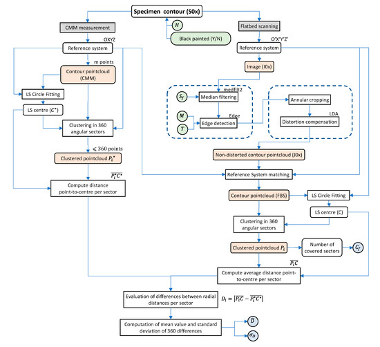
Figure 2.
Schematic flowchart of the experimental procedure.
2.1. Contrast Scenarios ()
Differences in contrast between the target contour and the surrounding background were expected to affect the results achieved by alternative combinations of image processing parameters. Contrast scenarios used in this research were generated modifying the part geometry or the background colour, while keeping illumination conditions constant. The reason was that, in the case of commercial FBSs, the lighting source is mounted on the scanner head and its angle of incidence is fixed by design. Additionally, the user does not commonly have total control upon image capture parameters, such as light intensity or exposure time. In fact, most commercial FBS software only allow image tuning after raw images have been captured.
In the case of extrusion additive manufactured (EAM) parts, geometry can affect contrast in three ways: firstly, the relative orientation of target contours with regard to the different sources of light present during scanning modifies the pattern of shadows and reflections; secondly, the distance between the target layer and the surrounding background (formed by all the previously-manufactured layers) also modifies the contrast pattern; thirdly, machine structures and part geometry can produce shadows and occlusions. To include contrast as a possible factor of influence, several considerations were made:
- To avoid contour-to-light relative orientation introducing bias in the analysis, a circular contour was selected as the test target. Light is directional in FBSs and no additional source of ambient light was present, therefore each possible angular relationship between normal-to-contour orientations and light direction was included in the test. This arrangement resembles a worst-case scenario in terms of contrast uniformity.
- Test specimens were designed to avoid interferences caused by structures or features in the surroundings of the objective contour.
- Due to the characteristics of FBS illumination, contrast increases when the distance between the top layer and the surrounding background increases. In this research, the height (H) of the layer that contains the target contour with respect to the background layer was used to generate different contrast scenarios (): (H = 8 mm), (H = 4 mm) and (H = 2 mm).
- An additional reference scenario (), presenting minimum contrast-dependant issues within the experiment was obtained by painting the background surface in matte black.
The circular contour selected as the test target was contained in the top layer of an inverted conical frustum, isolated in the middle of each test specimen (Figure 3). This design assured that no interference in the contrast pattern could be derived by nearby structures or geometrical features, whereas the FBS would be capable of digitising a neat view of the test target. The nominal diameter of the circumference () was set to 40 mm to properly apply the FBS local distortion adjustment (LDA) procedure described in [18]. A squared profile with chamfered corners was selected for the external shape of the specimens to fulfil reference and alignment requisites. All specimens were manufactured in 2.85 mm white BCN3D® PLA, with a BCN3D Sigma EAM machine, using the standard (0.1 mm layer resolution) manufacturing profile, as given by material’s supplier.
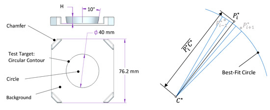
Figure 3.
Geometry and dimensions of test specimens (left) and schematic calculation of (right).
Differential characteristics of test specimens are presented in Table 1.

Table 1.
Experimental set characteristics.
2.2. Reference Characterisation of Specimen Geometry
Once manufactured, each test specimen was digitised using a coordinate measuring machine (CMM) DEA Global Image 09-15-08 with a contact touch-trigger probe. This machine was calibrated according to EN 10360-2:2001 being the maximum permissible error in length measurement as in (Equation (7)):
and the maximum permissible error in probing repeatability as in Equation (8):
A discrete point contact probing strategy registered the actual location of 360 contour points (), so that each 1° angular sector () is represented by a single point (Figure 3). Each point cloud was then adjusted to a circle using least squares to obtain the coordinates of the circle centre (). Then, the distance between each point and the circle centre was calculated (). Metrological operations regarding CMM digitising were performed using PC-DMIS®.
2.3. Acquisition and Processing of Target Images
Digital images of test targets were acquired using a Perfection V39 EPSON FBS. This model provides a working area of 216 mm × 297 mm. Each test specimen was placed upside-down, so that the last manufactured layer lay directly upon the glass. Scanning was carried out at 2400 dpi resolution along both sensor and scanning axes, and greyscale bitmap files () were obtained. An example of a raw image is provided in Figure 4a.
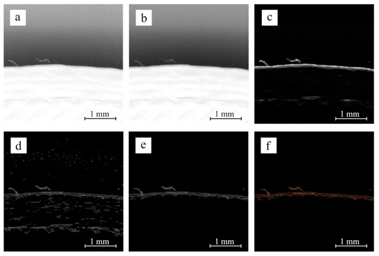
Figure 4.
Generalised example of consecutive steps in image processing: (a) raw image or ; (b) image after median filter; (c) image after applying differential operator; (d) image after thresholding; (e) image after annular cropping; (f) image () after LDA compensation.
Two steps of image processing were considered to define test factors: image filtering and edge detection. Image noise negatively influences discrete gradient computation [20]. Accordingly, filtering could affect the accuracy of contour characterisation. Digital images obtained from FBSs and other optical devices are frequently subjected to a “salt and pepper” noise type [28]. This noise could be caused by malfunctioning of pixel elements in the sensors, as well as by timing errors in the digitising [29] or related to flecks of dust inside the camera [30]. There are many filters that could be applied to remove this type of noise, but preparatory tests, as well as part of the results of previous researcher Balamurugan [31] led to the selection of a bi-dimensional median filtering stage as the first step in the image processing procedure.
FBS output images () were processed by means of MathWorks® function medfilt2 [32]:
This filter provided a transformed image (Figure 4b) where the value of each pixel has been substituted by the result of calculating a median filter in the -by- neighbourhood around the corresponding pixel. In the case of the present analysis, a square neighbourhood was considered, so a single value of filter size () was used to parameterise the filtering stage. It must be noted that only makes sense considering odd numbers, so that a regular matrix centred in the pixel is used for median calculation. Consequently, odd values between 1 and 59 were established as experimental levels for the factor.
Regarding edge detection, alternative approaches include methods based on the first derivative, second derivative and multi-step algorithms. Furthermore, the way these methods are implemented present slight differences when different digital image processing software is considered. In order to conduct a homogenous analysis, edge detection in this research was performed using the Edge function provided by MathWorks®. The Edge function is used to find edges in an intensity image, which is a data matrix that contains intensity values within a given range, corresponding each individual datum to an individual pixel [33]. The basic syntax of the Edge function can be seen in Equation (10) [34]:
where is a matrix of the same size as the input image () where each pixel adopts a value of 1 where the function identifies an edge point and a 0 value elsewhere. This function can be parameterised basically using two parameters: Method and Threshold.
- Method () is used to identify the specific edge-detection algorithm employed by the Edge function. Although this function uses the Sobel operator by default, it is possible to indicate an alternative method from a shortlist that includes first derivative operators (Roberts, Prewitt, Sobel), second derivate operators (LoG, ZeroCross) and two additional options based on Gaussian filtering approximation to the first derivative: Canny and ApproxCanny.
- Threshold () is a scalar used to discriminate between pixels and promote edge candidates to contour points. Those pixels with gradient intensity values above selected were identified as edge points, whereas those with a gradient intensity value below were ignored. When working with an 8-bit greyscale, 256 levels should be considered.
Nevertheless, in the case of the present work, variations of were sampled using multiples of 5 (from 0 to 250) to reduce the number of test combinations. The analysis of results would indicate whether a higher density of levels would be necessary in each scenario for a particular experimental range. If this were the case, an additional higher-density specific processing shall be performed. In the example given in Figure 4, the result of applying a differential operator is provided in Figure 4c, whereas the result of thresholding can be seen in Figure 4d.
In summary, three factors have been included in this research: the size of the median filter that is applied at first stage (), the edge-detection algorithm (), and the scalar value employed to perform the edge/null discrimination (). Tests were conducted using a full factorial; 9180 combinations of image processing factors (Table 2) have been tested for each contrast scenario.
Table 2.
Test factors and their correspondent experimental levels.
Each test combination for a given scenario provided a new image file containing white pixels (contour candidates) and black pixels. However, this image was subjected to two additional post-processing steps to refine the contour information: Annular Cropping and Local Distortion Adjustment (LDA).
The annular cropping has been specifically used here to remove unlikely contour candidates, taking advantage of the characteristics of this experimental design. The contour scan is subjected to the noisy influence of different hindrances, such as scratches, nap, dust particles or small wires of material caused by nozzle ooze. Additionally, odd elements related to the deposition path could also be mistaken for contour candidates (Figure 5).
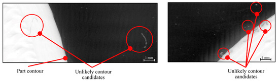
Figure 5.
Unlikely contour candidates derived from image hindrances and odd elements.
Fortunately, manufactured target contours are quite similar in size and shape to their corresponding theoretical definition (a circle). This allowed for the definition of a narrow annular area in the image within which the target contour should be contained. Subsequently, this area was used to crop the image and remove part of the unlikely contour candidates. To locate this annular area, a coarse approximation of the manufactured target diameter and the centre location in the image was obtained using a least-squares algorithm. Both approximate values were then used to define two concentric circles whose respective diameters differed by 1 mm (±0.5 mm with respect to the initial diameter approximation). The output of this step was a new digital image (Figure 4e). Although this “annular cropping” step was defined for this specific geometry, it could be easily adapted to different contours by defining the mask according to the correspondent nominal shape.
In the following step, LDA was applied to the coordinates of remaining contour points, so that the image distortion effect was compensated. A diffuse reflectance grid distortion target model 62-952—Edmund Optics—was used to characterise the distortion [18], decoupling its effect between sensor axis and scanning axis directions. This procedure minimises the influence of FBS local distortion on the target geometry, providing a new image of the undistorted contour candidates (Figure 4f).
2.4. Test Characterisation of Specimen Geometry
The resultant contour point cloud was then processed to extract geometrical information about the target that can be compared with the reference information provided by the CMM. An ideal circle was fitted using a least squares algorithm which provided a value for the diameter and the coordinates of its centre . Then, this information was used to cluster the points into 360 angular sectors. Given contour points clustered in sector , their average distance to was computed (Equation (11)).
2.5. Quality Indicators
Measurement quality indicators (MQIs) were used for evaluating the contour quality for each test combination and contrast scenario. The basis of this evaluation is a discrete comparison between the distance of contour points in sector to the centre of the target, under testing conditions (), and the corresponding reference distance calculated with the CMM. In this work, this comparison was achieved by means of the absolute difference between radial distances for each sector () (Equation (12)).
Three MQIs based on were then defined: coverage factor (), mean radial difference (), and standard deviation of the radial difference ().
- was defined as the percentage of angular sectors containing dimensional information (at least one valid contour point). If the processed image did not contain any contour point in a particular sector , then could not be calculated and this sector was excluded from the contour reconstruction. Accordingly, a higher value implied the higher completeness of test target reconstruction, and fewer possibilities of missing small contour abnormalities.
- was calculated as the mean value of all for a particular test. Accordingly, low values of indicated the location of contour points calculated under test conditions, such as those obtained with the CMM.
- represented the variability of along the contour. High values indicated that relative differences between correspondent FBS and CMM points varied along the contour.
2.6. Optimal Combination of Factors
In an ideal situation, selected MQIs would show an optimal behaviour for a unique combination of factors (, and ) in each contrast scenario (). Nevertheless, they were most likely expected to reach their correspondent optimal at different combinations of factors. To deal with this possibility, two alternative approaches to the optimisation problem were addressed: Coverage Priority and Accuracy Priority.
- Under the Coverage Priority approach, a combination of factors that provided the best coverage (ideally a 100% ) were extracted from the whole range of combinations. Then, smaller results were prioritised. If more than one candidate provided the maximum and the minimum among the reduced set, the combination that credited the minimum was finally selected.
- Under the Accuracy Priority approach, and results were arranged in 0.1 µm ranges. The algorithm sought first for combinations of factors that provided responses for both “accuracy” MQIs within the first range (e.g., ). An additional condition was imposed so that results would simultaneously provide at least a 75% coverage. If one or more combinations were found matching both conditions, the one with the maximum was chosen as the optimal combination. Nevertheless, if this were not possible, a second range (lower limit equal to the minimum response for each MQI and higher limit + 0.2 µm higher) would be explored, and the search would continue until at least one valid combination was found.
3. Results and Discussion
Variations in MQI values between different combination of test parameters (, and ) for each contrast scenario will be presented and discussed independently. Differences between contrast scenarios will also be analysed and discussed.
The direct relationship between and the contrast can be clearly observed in the raw images () captured with the FBS for each scenario (Figure 6).
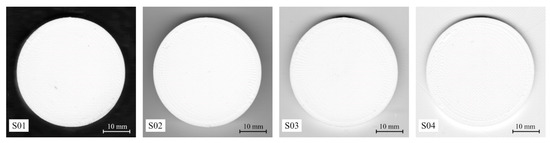
Figure 6.
Raw images () captured for , , and contrast scenarios.
As was expected, showed the sharpest contrast between the test target and the background. also presented a clear and uniform contrast even when, although was the same as in , its background had not been painted in black. For lower ( and ), greyscale differences between the background and the top layer decreased. Moreover, lower sectors of the test contour presented a reduced local contrast because FBS directional illumination arrangement increased background brightness; simultaneously, upper sectors kept an appreciable contrast because the top layer cast a clear shadow upon the background. Test specimens showed a symmetric 180° behaviour between normal-to-contour vectors and the illumination direction.
3.1. Analysis of Contour Reconstruction Reliability for
Distribution of , and results as a function of and corresponding to the scenario is presented in Figure 7. Each row in Figure 7 contains three graphs corresponding to the same edge detection method (), corresponding each one to each MQI (, or ). Each graph represents the distribution of its MQI values with respect to the filter size () and the threshold () by means of a colour scale. Thus, cooler colours represent better relative results than warmer colours. Figure 6 shows that all MQI showed high dependence on and , whereas certain similarities were observed between different methods.
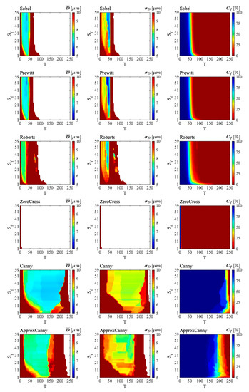
Figure 7.
Measurement quality indicator (MQI) results as a function of and for every calculated for .
Variations in results distribution regarding and were quite similar among first derivative methods (Sobel, Prewitt and Roberts). These methods showed a high dependence of with respect to . Medium-to-high values severely reduced the contour coverage, except for several test combinations with extremely low values. Severe coverage drops were observed for , while was found to be far less sensitive to changes in . and also worsened for high values, but this does not mean that best accuracy results corresponded to extremely low values. In fact, a narrow interval of intermediate values provided minimum and results, which implied the best similarity between the FBS digitising and the CMM reference. These intervals were wider and more homogeneous in the case of , and thinner and more -dependent in the case of .
Both Canny and ApproxCanny methods presented a broad range of and combinations providing a complete coverage of the test target contour. Nevertheless, showed minimum values for Canny when intermediate and were selected. For a given value, combinations with extremely high or low values provided poor results. Nonetheless, was found to be also sensitive to variations for a given , although this effect was less noticeable for intermediate values. A similar behaviour was observed regarding . ApproxCanny, on the other hand, presented better and results for combinations of intermediate and high values. The interval of optimal combinations was narrower here than it was for Canny but was still far wider than the one observed in first derivative methods.
Finally, ZeroCross showed a completely different distribution of results because, for the original test resolution, it seemed that no valid results could be achieved for combinations (Figure 7). Moreover, even for , the coverage was very poor. Nevertheless, coverage was not the only problem with this method, because even optimal and results were very poor. It seemed that ZeroCross should be rejected, therefore these results were confined to such a small range of that a second round of the test was performed in the experimental range with a sample step (Figure 8).
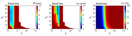
Figure 8.
MQI results as a function of calculated with ZeroCross for in a reduced range.
Accordingly, ZeroCross was far more sensitive to values than other methods. Slight variations in caused quality results to vary abruptly. Conversely, an adequate selection of and provided excellent results which, in certain cases, could be even adopted for an optimal contour characterisation. Thus, combinations with and provided a good coverage and very low and values.
Overall results showed that an appropriate selection of and was required to achieve the best coverage and accuracy results. If a complete coverage was prioritised against accuracy, it could be achieved under many test combinations. Nevertheless, only a small fraction of such combinations would simultaneously provide the lower range of and values.
Simultaneous optimisation under both coverage priority and accuracy priority criteria was not possible for almost all tested edge-detection methods (Table 3). In fact, only the Canny method provided a combination of and () leading simultaneously to the best results of (100%), (6.65 µm) and (7.65 µm). Nevertheless, Canny would not be the best option for the scenario, because ApproxCanny provided a slightly lower value (7.50 µm) under the coverage priority criterion, and Prewitt provided better results under the accuracy priority criterion ().
Table 3.
Optimal combinations of test parameters for .
3.2. Analysis of Contour Reconstruction Reliability for
Results variations between and scenarios were exclusively related to contrast differences because, although both specimens shared the same dimensions, only had its background painted in black. All quality indicators showed a high dependence on , while had a lower, but not negligible, influence (Figure 9). Nevertheless, overall results were clearly worse than those obtained for . This result was common to all the edge-detection methods tested, indicating that the reduction in contrast had a direct impact on the quality of contour characterisation.
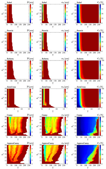
Figure 9.
MQI results as a function of Sf and T for every M calculated for .
Thus, the range of values providing 100% was thinner independent of the method used, and a significant reduction in and was also found for equivalent test combinations between and . Nevertheless, the observed worsening of results was less noticeable in the case of Canny and ApproxCanny methods.
Under the coverage priority criterion (Table 4), the best achievable results for worsened the equivalent results for . Only Canny provided results that, although still worse, could be compared to those obtained for . On the other hand, assuming a slight reduction in under the accuracy priority criterion, would improve and . This was especially relevant in the case of ZeroCross, Canny and ApproxCanny methods. For example, in the case of the Canny method, a and combination reduced to 7.52 µm and to 6.77 µm while keeping 99.44% . ZeroCross would be the preferable option under this criterion, because an and combination achieved and . These results reinforced the idea that an a priori selection of processing conditions is a sine qua non condition to achieve reliable results.
Table 4.
Optimal combinations of test parameters for .
S02 showed a clear reduction in the range of adequate test combinations when using Canny. To clarify this circumstance, Figure 10 contains samples of contour points obtained with Canny for three different test combinations: T15/Sf39, T40/Sf39 and T75/Sf39.
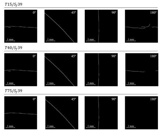
Figure 10.
Samples of S02 contour points obtained with Canny for different angular positions and test configurations: T15/Sf39 (upper row), T40/Sf39 and T75/Sf39 (lower row).
The optimal combination under the accuracy priority criterion () provided clearly defined lines, although a small segment corresponding to a double contour can be observed in the 0° orientation sample and a small area without points was observed in the 180° orientation sample (Figure 10). These extracted contours provided excellent results in terms of coverage and accuracy (Table 4). Reducing () increased up to 14.97 µm, and up to 8.56 µm while simultaneously reaching a full coverage. Coverage improvement was achieved through an increment of multiple-contour detection issues (180° orientation in Figure 10) which, on the other hand, reduced the overall accuracy. Using a higher threshold (), however, minimised multiple contour detection issues, at the cost of a lower coverage (), which can be noticed in the complete loss of contour information around the 180° orientation.
To better explain differences between the selected combinations, Figure 11 provides polar plots of the radial differences () between the measured radial position of each sector and the nominal radius (). Each polar plot contains this information calculated for the reference CMM-measured radial distances () and for the FBS-measured radial distances obtained with a particular test factor combination ().
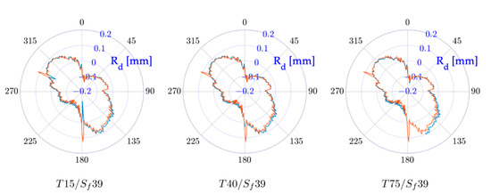
Figure 11.
Polar graphs of calculated for including reference CMM data (red dots) and three different test conditions (blue dots).
Figure 11 reveals that major differences occurred in two specific orientations: 180° and 293°. Regarding the 180° orientation, the original image () reveals an abnormality in contour that was part of a seam feature on the 3D geometry (Figure 12).
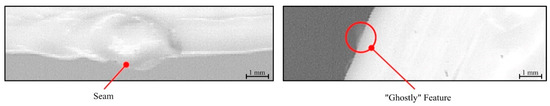
Figure 12.
Samples of original scans showing a seam in the 180° orientation (left) and a “ghostly” feature in the 293° orientation (right).
Seams are common features in the AM extrusion of thermoplastics, related to points “where a new deposition path starts or ends” [34]. The CMM correctly traces the contour of the seam, which appears as a positive deviation with respect to the surrounding contour. On the other hand, the FBS-based contour detection does not correctly trace this feature under those configurations included in Figure 10 and Figure 11. This circumstance can be attributed to local contrast variations, because the local geometry of the seam showed a very different aspect from the surrounding contour. Accordingly, it is difficult that a unique image processing configuration works properly with both the seam feature and the closer segments of contour. On the other hand, the 293° orientation provided an outstanding value registered with the CMM, caused by a feature below the target layer. This “ghostly” feature has been previously observed [18] and described as “small protuberances” located too close to the top layer, so that they are registered by the CMM touch probe. In this case, the FBS-based analysis correctly ignored this protuberance, showing more robustness against “ghostly” features than the CMM. In any case, a robust contour-detection procedure must be aware of the possible presence of these abnormalities and apply adequate treatments to avoid their negative influence on contour reconstruction.
Finally, the relevance of the annular cropping strategy can be observed in Figure 13.
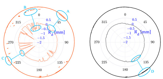
Figure 13.
Polar graphs for using a test combination: without annular cropping (left) and with annular cropping (right).
Processing the whole image with a combination provided several unlikely contour candidates. These segments could be located inside the top layer, such as A or B details, or in the background, such as detail C (Figure 13). Although this combination did only introduce few unlikely contour candidates without annular cropping, they had a huge influence on MQI results (Table 5).
Table 5.
MQI results for using a test combination without annular cropping and with annular cropping.
At the same time, the large segment in detail A reduced the apparent of its corresponding sectors. A similar, discontinuous phenomenon is present in detail B. On the other hand, the small segment in detail B artificially enlarged . When annular cropping was applied (Figure 13, right), the effect of such localised errors was minimised, although not completely removed. For example, the detail D shows a multi-contour issue that lies inside the remaining area after the annular cropping step, and its effect on can be clearly seen. Contrary to the usual situation when recognising contours on digital images, the specific characteristics of AM layer contour characterisation allow for an a priori coarse approximation of the test target location in the image. Accordingly, this approximation could be used to generate a reduced area of interest, cropping the rest of the image, and avoiding external features to introduce noise during contour characterisation. The FBS-based contour characterisation of AM layers should take advantage of this particularity, as it was the case of the analysis presented here.
3.3. Analysis of Contour Reconstruction Reliability for
Quality indicators worsened for , independent of which edge-detection method had been applied. Coverage results dropped with respect to the previous scenarios, so that only Approxcanny or Canny methods provided a high range of and combinations that achieved 100% . Worsening of contour characterisation quality was also observed. In fact, results were so poor that the 5–10 µm colour scale used for the first two specimens had to be substituted by a 10–100 µm scale (Figure 14).
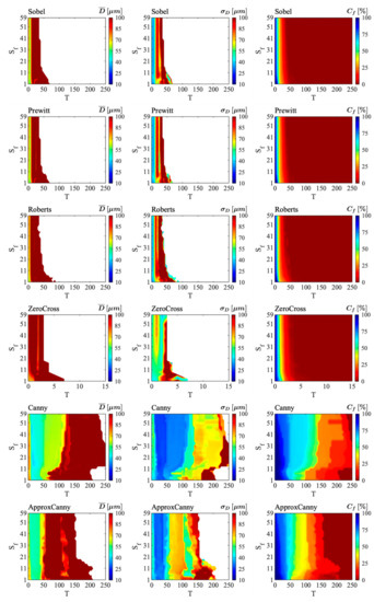
Figure 14.
MQI results as a function of and for every calculated for .
Observed variations in and were not as sharp as those observed in , but their response to or variations was quite similar: high values worsened and results, whereas did not to have a significant influence.
Reduction in high-quality combinations influenced the differences observed between coverage priority and accuracy priority. In fact, results were quite similar under both criteria, apart from Canny and ZeroCross. In fact, ZeroCross showed a noticeable reduction in (100% under coverage priority against 9.72% under accuracy priority). Roberts would be the recommendation here for an optimal scan under the coverage priority criterion, whereas Canny would be selected under the accuracy priority criterion (Table 6). Nevertheless, the minimum value was 25.81 µm (Canny; ; ), which is nearly four times higher than the best result obtained for . Similarly, the minimum value was 42.06 µm for the same configuration, which is more than five times higher than the optimal for . These results indicate that using an optimal processing configuration was critical, because there were fewer adequate combinations. Moreover, even when optimal combinations were applied, results were several times worse than those observed in sharper and more uniform contrast scenarios.
Table 6.
Optimal combinations of test parameters for .
To discuss possible causes of this overall worsening, Figure 15 contains samples of contour points obtained with Canny for three different test combinations: , and .
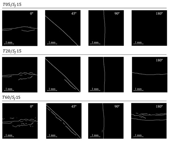
Figure 15.
Samples of contour points obtained with Canny for different angular positions and test configurations: (upper row), and (lower row).
The optimal combination under the accuracy priority criterion () provided clear contour lines for 90° and 180° orientations, but failed to remove multiple-contour detection issues for 0° and 45° orientations (Figure 16). Therefore, although providing a reasonably good coverage, accuracy indicators were noticeably worse than those achieved for (Table 4 and Table 6). Lower thresholds severely increased the multiple-contour detection because the algorithm registered many weak gradients as contour candidates. This circumstance allowed for achieving a full coverage but worsened other indicators. Increased threshold reduced the number of multiple-contour issues, although it did not provide a complete suppression as can be observed for the 0° orientation in Figure 15. Nevertheless, it also removes large sectors (180°) that were accurately reconstructed at lower threshold. These effects can be also observed through the polar plots of the radial differences () presented in Figure 16.
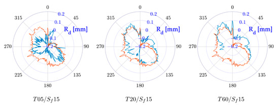
Figure 16.
Polar graphs of calculated for including reference CMM data (red dots) and three different test conditions (blue dots).
Polar graphs illustrate how multiple-contour detection issues negatively affect the contour reconstruction accuracy (Figure 16). At lower T, the algorithm included comparatively weak gradients as contour candidates, causing the existence of multiple-contour candidates within the same angular sector and allowing a full contour coverage. When T increased, fewer multiple-contour issues occurred, but several sectors did not provide any valid contour point. This phenomenon is directly linked to a higher , causing the loss of a larger sector (nearly 120° for ) and rendering contour reconstruction useless. Nevertheless, this loss of information was not randomly distributed along the contour. In fact, only lower sectors were affected while upper sectors retained an adequate coverage despite growing .
This circumstance suggested that the observed behaviour was related to an anisotropic phenomenon. Consequently, the lack of uniformity in contrast between the target contour and the surrounding background regarding local contour orientation was thereafter analysed (Figure 17).
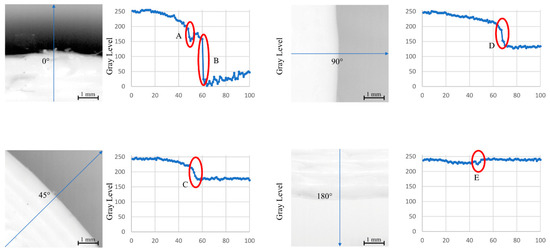
Figure 17.
Linear samples of grey-level intensity distribution in the original scan of for different orientations: 0° (top left); 45° (bottom left); 90° (top right); 180° (bottom right).
Linear samples of grey-level intensity distribution in the original are presented in Figure 17. In two of those orientations (45° and 90°) there were clearly defined isolated greyscale transitions (details C and D). Conversely, other orientations reveal multi-transition issues (details A and B in 0° orientation) and weak transition issues (detail E in 180° orientation). Accordingly, a relevant anisotropic behaviour of contrast was present. The FBS directional illumination brightened background areas next to the lower sectors of the target contour. Simultaneously, the 3D geometry cast a shadow in the background areas next to the upper sectors. Intermediate orientations showed an intermediate behaviour. Accordingly, the contrast anisotropy caused an evident lack of uniformity of greyscale transitions. This phenomenon was not just restricted to the contour itself, but also caused variations in the local grey intensity of the upper layer related to manufacturing characteristics (deposited material topography) and defects (seams). Multiple transitions caused multi-contour detection issues. These transitions must present certain differences (contour transition should be sharper than the rest, see A and B details), therefore lower T values would not properly discriminate them. On the other hand, using higher T values to minimise this problem would neglect low-contrasted contour sectors (see detail E). Due to T being the same for the whole image, contrast anisotropy was a major issue for the contour reconstruction. Arguably, the higher the anisotropic behaviour of contrast in the whole contour, the harder it is for an edge-detection algorithm to provide an appropriate reconstruction.
3.4. Analysis of Contour Reconstruction Reliability for
This scenario provided the lower contrast (considering the test target as a whole) within the limits of the present work (Figure 18). Moreover, it also provides greatest local differences in contrast, because the FBS illumination introduced a noticeable reflection in the neighbourhood of the lower arc and, at the same time, originated a shadow near the upper arc.
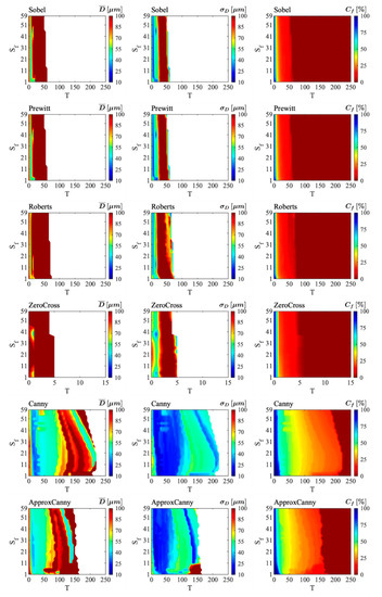
Figure 18.
MQI results as a function of and T for every M calculated for S04.
The best coverage was obtained for extremely low values (Figure 18). In fact, just a narrow interval of combinations provided full coverage, with the only exception of some and combinations with extremely low in the case of Canny and ApproxCanny methods. Nevertheless, results were very poor for this scenario, when compared with the previous situations. A compromise between coverage and accuracy could hardly be achieved because best coverage implied very poor and results. In the case of first derivative algorithms, 100% increased over 100 µm, whereas was always above 55 µm. A similar situation was observed regarding ZeroCross. In the mentioned cases, a full coverage could only be achieved using , which implied a high sensitivity to weak gradients. The consequence, as it was described before, was a multi-contour detection issue that was directly related to poor accuracy results. On the other hand, although Canny and ApproxCanny improved these, results were still poor, such as those obtained for .
The best and results were achieved with test combinations that provided very poor coverage (below the minimum 75%). This scenario also showed a highly anisotropic contrast, therefore it presented an even worse compromise between coverage and accuracy than . Thus, coverage dramatically dropped with growing , and the number of valid combinations under the condition was low, except for Canny and ApproxCanny methods. Nevertheless, even those methods presented deviations ranging tens of microns, which made them unsuitable for feasible contour characterisation.
Under the coverage priority criterion (Table 6), the optimal combination used Canny, and (). Under the accuracy priority criterion, the optimal combination also used Canny, and () (Table 7).
Table 7.
Optimal combinations of test parameters for .
3.5. Minimising the Effect of Contrast Lack-Of-Uniformity: Proposed Approaches
Contrast characteristics showed a high influence upon contour reconstruction accuracy. Lack of uniformity in contrast between the test target and its surrounding background was directly related to poor results. This lack of uniformity was related to the directional illumination in the FBS, causing an anisotropic distribution of bright-ened and shadowed areas in the background. In this test design, worsening of results caused by contrast anisotropy was directly related to the distance between the target layer and the background (H). Accordingly, if H was large enough (the case of S02), FBS illumination did not reach the background with enough intensity to generate highly anisotropic brightness and shadow patterns. In this situation, background illu-mination was more uniform, and this caused a smoother appearance. The explanation of this behaviour is related to tested edge-detection algorithms because they use a threshold (T) value to promote image points to contour points. This approach is clearly not adequate when the intensity gradients present non-uniform characteristics, because of contrast anisotropy. This phenomenon can be affected by the presence of abnormal features, such as seams or oozing, causing local contour reconstruction discontinuities or locally reducing its accuracy. Moreover, results could be even worse if the vertical distance between the contour and the background is not constant. Accordingly, tested edge-detection algorithms should only be used for AM contour characterisation in ar-rangements with uniform contrast between the background and layer. This also means that a robust FBS-based OMM verification procedure of AM layers must include ele-ments that minimise the influence of contrast anisotropy. We propose two possible approaches to deal with this problem in the future: a uniform contrast approach and adaptive edge-detection.
- A uniform contrast approach would consist of a combination of illumination arrangements and image processing, tailored to assure that each contour segment presented similar contrast characteristics. A possible arrangement would imply consecutive scans of the contour using different relative orientations between part and light direction, and merging those specific areas where contrast characteristics were similar. This approach would affect the physical system, because an additional degree of freedom between part and sensor should be considered. Additionally, it also complicates image processing, because it would be necessary to relate all scans to the same reference system, to cluster normal-to-contour orientations, to remove areas with inappropriate contrast characteristics, and to merge remaining areas into a single image. Finally, it is not clear that this approach could provide an adequate solution to the problem of local contour abnormalities.
- Adaptive edge-detection would involve particularising edge detection as a func-tion of local contrast characteristics for different contour segments. This particu-larisation should consider local greyscale transition characteristics in the vicinity of a contour point candidate. The approximate location of the contour would be known, therefore a function that selects an optimal T considering the contour orientation and the layer-to-background distance would provide an adequate response to anisotropic contrast. This approach does not af-fect the physical system, nor demands multiple scans. Nevertheless, it requires a mathematical model that includes all possible factors influencing contrast ani-sotropy, such as the distance to the background, the contour orientation or the op-tical characteristics of material. This requirement would imply an additional cal-ibration step, that could include a specific treatment for local abnormalities.
4. Conclusions
Flatbed scanning has proven to be an adequate and reliable digitising method, suitable for AM contour characterisation, in those situations where contrast variability between the contour and the background is low. In such situations, the quality of contour characterisation is highly dependent on image processing parameters. An adequate combination of filtering and edge-detection parameters has a significant influence upon observed results. Edge-detection method (M), threshold (T), and filter size (Sf) must be carefully selected to achieve the best results. It was also observed that it is not possible to simultaneously obtain the best achievable results of the coverage factor (Cf) the mean radial difference (), and the standard deviation of the radial difference (σD) using a single image processing configuration. Accordingly, a compromise between coverage and accuracy must be observed. Two alternative approaches have been proposed: coverage priority and accuracy priority. Both approaches could be adjusted to match specific requirements in terms of coverage or accuracy, within the limits observed in this research.
It has been also proven that the contour detection is highly dependent on the contrast uniformity between the target contour and the background. A uniform contrast is related to the lower variability of local gradients, enabling the accurate identification of the contour points using a unique T value. Although providing a strict recommendation would maybe be too ambitious, results from S01 and S02 indicate that using the Canny method with high Sf values (Sf > 31) and fixing a T = 40 threshold would provide almost full contour coverage (Cf > 99%), while keeping low values for the other indicators (). These combinations could be used as a reference when processing uniform and highly contrasted contours.
On the other hand, when contrast shows an anisotropic distribution along the contour, the compromise between coverage and accuracy becomes unbalanced, and contour characterisation turns unfeasible. Non-uniform brightness and shadow patterns, caused by a reduction in layer-to-background distance, severely influence contour detection. In these situations, because the algorithms use a unique T for processing the whole image, low T values will provide good coverage and poor accuracy, whereas increasing T will progressively decrease coverage and slightly increase accuracy. Although Canny and ApproxCanny methods have shown higher robustness on contrast issues than first derivative algorithms or ZeroCross, the described procedure would not be adequate for highly anisotropic scans.
A robust FBS-based OMM verification procedure of AM layers should minimise the influence of contrast anisotropy. We propose that future developments adopt a uniform contrast approach or an adaptive edge-detection approach. A uniform contrast approach would demand a combination of illumination arrangement and image processing to process contour segments with similar contrast characteristics. Adaptive edge-detection would require a new edge-detection procedure that considers local contrast characteristics and influence factors, such as the distance to the background as a function of the geometry of previous layers, the contour orientation, or the optical characteristics of material.
An additional conclusion is that local abnormalities should demand a specific treatment during contour extraction and analysis because they have a significant influence upon the overall results. These anomalies are not derived from a lack of mechanical accuracy or deviations in contour path tracing, but from specific errors or deficiencies on the material extrusion dynamics. Accordingly, when an excessive accumulation of material (e.g., seams) or out-of-contour material (e.g., oozing phenomenon) appear, a robust procedure must detect them and apply a specific treatment.
Finally, the strategy of applying an annular crop has been found useful to reduce inaccurate identification of contours. We suggest that any approach pursuing AM layer contour characterisation should use a similar strategy, using an approximation to the contour location extracted from the CAD or the STL files to generate a mask that removes areas of the scan that do not contain information about the contour geometry.
These findings should be carefully considered in future attempts to use FBS for metrological assessment of AM layer geometry, because our results have proved that both the selection of image processing configuration and the contrast pattern have a significant influence on the accuracy of contour reconstruction.
Author Contributions
Conceptualization, D.B.; Data curation, A.F. and B.J.A.; Formal analysis, B.J.A.; Funding acquisition, J.C.R.; Investigation, P.F. and J.C.R.; Methodology, P.F.; Project administration, D.B.; Software, P.F. and A.F.; Supervision, D.B. and J.C.R.; Validation, D.B.; Visualization, A.F.; Writing – original draft, D.B.; Writing – review & editing, D.B., P.F., A.F., B.J.A. and J.C.R. All authors have read and agreed to the published version of the manuscript.
Funding
Ministerio de Economía, Industria y Competitividad, Gobierno de España: DPI2017-83068-P.
Institutional Review Board Statement
Not applicable.
Informed Consent Statement
Not applicable.
Data Availability Statement
Data sharing not applicable.
Acknowledgments
This work was supported by the Spanish Ministry of Economy, Industry and Competitiveness and by FEDER (DPI2017-83068-P).
Conflicts of Interest
The authors declare no conflict of interest.
References
- Basiliere, P.; Shanler, M. Hype Cycle for 3D Printing; Gartner Inc.: Stamford, CT, USA, 2019. [Google Scholar]
- Wohlers, T. Wholers Report 2012—Additive Manufacturing and 3D Printing State of the Industry; Annual Worldwide Progress Report; Wholers Associates: Fort Collins, CO, USA, 2012. [Google Scholar]
- Noriega, A.; Blanco, D.; Alvarez, B.J.; Garcia, A. Dimensional Accuracy Improvement of FDM Square Cross-Section Parts Using Artificial Neural Networks and an Optimization Algorithm. Int. J. Adv. Manuf. Technol. 2013, 69, 2301–2313. [Google Scholar] [CrossRef]
- Boschetto, A.; Bottini, L. Triangular mesh offset aiming to enhance Fused Deposition Modeling accuracy. Int. J. Adv. Manuf. Technol. 2015, 80, 99–111. [Google Scholar] [CrossRef]
- Skala, V.; Pan, R.; Nedved, O. Making 3D Replicas Using a Flatbed Scanner and a 3D Printer. Computational Science and Its Applications—ICCSA 2014. Lect. Notes Comput. Sci. 2014, 8584, 76–86. [Google Scholar] [CrossRef]
- Valiño, G.; Rico, J.C.; Fernández, P.; Álvarez, B.J.; Fernández, Y. Capability of conoscopic holography for digitizing and measuring of layer thickness on PLA parts built by FFF. Procedia Manuf. 2019, 41, 129–136. [Google Scholar] [CrossRef]
- Phuc, L.T.; Seita, M. A high-resolution and large field-of-view scanner for in-line characterization of powder bed defects during additive manufacturing. Mater. Des. 2019, 164, 107562. [Google Scholar] [CrossRef]
- Tang, Z.; Liu, W.; Zhang, N.; Wang, Y.; Zhang, H. Real–time prediction of penetration depths of laser surface melting based on coaxial visual monitoring. Opt. Lasers Eng. 2020, 128, 106034. [Google Scholar] [CrossRef]
- Syam, W.P.; Rybalcenko, K.; Gaio, A.; Crabtree, J.; Leach, R.K. Methodology for the development of in-line optical surface measuring instruments with a case study for additive surface finishing. Opt. Lasers Eng. 2019, 121, 271–288. [Google Scholar] [CrossRef]
- Dalen, G.V. Determination of the size distribution and percentage of broken kernels of rice using flatbed scanning and image analysis. Food Res. Int. 2004, 37, 51–58. [Google Scholar] [CrossRef]
- Kee, C.W.; Ratman, M.M. A simple approach to fine wire diameter measurement using a high-resolution flatbed scanner. Int. J. Adv. Manuf. Technol. 2009, 40, 940–947. [Google Scholar] [CrossRef]
- Poliakow, E.V.; Poliakov, V.V.; Fedotova, L.A.; Tsvetkov, M.K. High.-Precision Measuring Scale Rulers for Flatbed Scanners; Astronomy and Space Science; Heron Press Ltd.: Sofia, Bulgaria, 2007. [Google Scholar]
- Kangasrääsiö, J.; Hemming, B. Calibration of a flatbed scanner for traceable paper area measurement. Meas. Sci. Technol. 2009, 20, 1–4. [Google Scholar] [CrossRef]
- Wyatt, M.; Nave, G. Evaluation of resolution and periodic errors of a flatbed scanner used for digitizing spectroscopic photographic plates. Appl. Opt. 2017, 56, 3744–3749. [Google Scholar] [CrossRef] [PubMed]
- Jones, M.P.; Callahan, R.N.; Bruce, R.D. Dimensional Measurement Variation of Scanned Objects Using Flatbed Scanners. J. Technol. Manag. Appl. Eng. 2012, 28, 2–12. [Google Scholar]
- De Vicente, J.; Sanchez-Perez, A.M.; Maresca, P.; Caja, J.; Gomez, E. A model to transform a commercial flatbed scanner into a two-coordinates measuring machine. Measurement 2015, 73, 304–312. [Google Scholar] [CrossRef]
- Majarena, A.C.; Aguilar, J.J.; Santolaria, J. Development of an error compensation case study for 3D printers. Procedia Manuf. 2017, 13, 864–871. [Google Scholar] [CrossRef]
- Blanco, D.; Fernandez, P.; Noriega, A.; Alvarez, B.J.; Valiño, G. Layer Contour Verification in Additive Manufacturing by Means of Commercial Flatbed Scanners. Sensors 2020, 20, 1. [Google Scholar] [CrossRef]
- Solomon, C.; Breckon, T. Fundamentals of Digital Image Processing; John Wiley & Sons, Ltd.: West Sussex, UK, 2011. [Google Scholar]
- Jain, R.; Kasturi, R.; Schunck, B.G. Machine Vision; McGraw-Hill, Inc.: New York, NY, USA, 1995; ISBN 0-07-032018-7. [Google Scholar]
- Papari, G.; Petkov, N. Edge and line oriented Contour detection: State of the art. Image Vis. Comput. 2011, 29, 70–103. [Google Scholar] [CrossRef]
- Gong, X.-Y.; Su, H.; Xu, D.; Zhang, Z.-T.; Shen, F.; Yang, H.-B. An Overview of Contour Detection Approaches. Int. J. Autom. Comput. 2018, 15, 656–672. [Google Scholar] [CrossRef]
- Spontón, H.; Cardelino, J. A Review of Classic Edge Detectors. Image Process. Line 2015, 5, 90–123. [Google Scholar] [CrossRef]
- Roberts, L.G. Machine Perception of Three-Dimensional Solids. Ph.D. Thesis, Massachusetts. Institute of Technology, Cambridge, MA, USA, 1963. [Google Scholar]
- Duda, R.; Hart, P. Pattern Classification and Scene Analysis; John Wiley & Sons Inc.: Hoboken, NJ, USA, 1973; ISBN 0471223611. [Google Scholar]
- Prewitt, J.M.S. Object enhancement and extraction. In Picture Processing and Psychopictorics; Lipkin, B.S., Rosenfeld, A., Eds.; Academic Press: Hoboken, NJ, USA, 1970; pp. 75–149. ISBN 9780323146852. [Google Scholar]
- Cuevas, E.; Zaldivar, D.; Pérez, M. Procesamiento digital de imágenes con MatLAB y SIMULINK; Alfaomega & RA-MA: Mexico D.F., Mexico, 2010; ISBN 978-6077070306. [Google Scholar]
- Mamatha, H.R.; Madireddi, S.; Murthy, S. Performance analysis of various filters for De-noising of Handwritten Kannada documents. Int. J. Comput. Appl. 2012, 48, 29–37. [Google Scholar] [CrossRef]
- Saxena, C.; Kourav, D. Noises and Image Denoising Techniques: A Brief Survey. Int. J. Emerg. Technol. Adv. Eng. 2014, 4, 878–885. [Google Scholar]
- Garg, R.; Kumar, A. Comparison of various noise removals using bayesian framework. Int. J. Mod. Eng. Res. 2012, 2, 265–270. [Google Scholar]
- Balamurugan, E.; Sengottuvelan, P.; Sangeetha, K. An Empirical Evaluation of Salt and Pepper Noise Removal for Document Images using Median Filter. Int. J. Comput. Appl. 2013, 82, 17–20. [Google Scholar] [CrossRef]
- The Mathworks Inc. MathWorks.com Online. Available online: https://www.mathworks.com/help/images/ref/edge.html (accessed on 1 March 2020).
- Gonzalez, R.C.; Woods, R.E.; Eddins, S.L. Digital Image Processing Using Matlab®, 2nd ed.; Gatesmark Publishing: Knoxville, TN, USA, 2009; ISBN 0982085400. [Google Scholar]
- Brischetto, S.; Maggiore, P.; Ferro, C.G. Additive Manufacturing Technologies and Applications; MDPI AG: Basel, Switzerland, 2017; ISBN 978-3-03842-548-9. [Google Scholar]
Publisher’s Note: MDPI stays neutral with regard to jurisdictional claims in published maps and institutional affiliations. |
© 2020 by the authors. Licensee MDPI, Basel, Switzerland. This article is an open access article distributed under the terms and conditions of the Creative Commons Attribution (CC BY) license (http://creativecommons.org/licenses/by/4.0/).