Abstract
One of the challenges in predicting the remaining useful life (RUL) of rolling element bearings (REBs) is determining a proper failure threshold (FT). In the literature, the FT is usually assumed to be a constant value of an extracted feature from the vibration signals. In this study, a degradation indicator was extracted to describe damage to REBs by applying principal component analysis (PCA) to their run-to-failure data. The relationship between this degradation indicator and the vibration peak was represented through a joint probability distribution using statistical copula models. The FT was proposed as a probability distribution based on the fluctuation increase in the vibration trend. A set of run-to-failure tests was conducted. Applying the proposed method to this dataset led to various FTs for the different failure modes that occurred. It is shown that, for inner race degradation, a higher FT can be assumed than for rolling element degradation. This could help extend the lives of REBs regarding the degrading elements. A dataset for an industrial machine was also analyzed and it is shown that the proposed model estimated a reasonable and proper FT in an actual case study.
1. Introduction
Rolling element bearings (REBs) are one of the most common mechanical components of rotary machines. The failure of these components is the main reason for 45% to 55% of machines breakdown [1]. This is why researchers have paid more attention to predicting the remaining useful life (RUL) of REBs over the past two decades. The RUL of REBs is defined as the remaining time until a vibration feature reaches the predetermined failure threshold (FT) [2], which is often assumed to be a constant value in the literature. Therefore, the accuracy of the RUL prediction depends on selecting a proper FT. Furthermore, the determination of FTs for various vibration features is a challenging issue. In general, to achieve protective or predictive goals in preventing the breakdown of rotary machines, the FT is determined experimentally, based on the manufacturers′ recommendation or using the recommendations of standard codes (e.g., ISO 10816-3 [3]). The recommendations in ISO 10816-3 and other similar codes correspond to different fault types in machines in the frequency range of 10 to 1000 Hz. They are thus not specifically for the failure of REBs. Therefore, employing a suitable and proper FT for REBs leads to the more reliable and economical operation of rotary machines.
Reviewing the literature, three different approaches can be considered for defining the FT: (1) as a constant value of a vibration feature, (2) as a probability distribution of a vibration feature or (3) as a specific level of physical damage. In most research studies on the RUL prediction of REBs, the FT is defined as a constant value of a vibration feature (e.g., the root mean square (RMS) or the time signal entropy) [4,5,6,7,8]. This approach is the most convenient method for this issue. For instance, in the PRONOSTIA dataset [9], which is a set of run-to-failure tests of REBs conducted by the FEMTO-ST institute in 2011, the constant value of the vibration peak (20 g) was employed as the stop criterion of the tests. After the publication of this dataset at the PHM 2012 conference, many researchers used it to validate their studies [10,11,12]. Most of them have used the test stop criterion as the FT in their RUL prediction problems.
In the second approach, the FT is defined as a probability distribution of a vibration feature. This approach has been widely used in reliability literature. In this regard, Wang and Coit [13] studied the effect of different FT distributions on equipment reliability. Nystad et al. [14] used the gamma distribution of the degradation indicator for the FT, the parameters of which were determined by experts, to estimate the probability of chock valves’ RUL accurately. In another study, Yu and Fuh [15] studied the failure of an element in the crack propagation problem. They proposed a probability distribution of the crack size to define a failure threshold in the fatigue test results.
Using a specific level of physical damage as a FT is less common than the previous approaches. Another dataset that has been employed in the RUL prediction literature is that of the REB run-to-failure tests conducted by the Center for Intelligent Maintenance Systems (IMS) at the University of Cincinnati [16]. In this dataset, the test stopping criterion was defined as a specific contaminant level in the REB lubrication feedback system. Reaching this level led to the activation of an electrical switch that stopped the test running. The dataset included three run-to-failure experiments on four similar parallel REBs mounted on a single shaft. These experiments stopped with the same physical damage criterion, which was explained earlier. However, investigating the results of the vibration records revealed a significant difference between the levels of various vibration features at the end of these three tests. This means that the stopping criterion in this dataset employed led to extremely different results from the first approach, which was explained earlier. Some researchers [17,18] have used the stopping criteria of these tests as the FT in their studies on the IMS dataset. However, others [19,20] have employed a constant value of the vibration features as the FT in IMS tests. Therefore, the end of life (EoL) may differ from the end of the test in these studies.
Reviewing the literature, it can be seen that the details of defining a proper FT were less extensively considered in the RUL prediction of REBs. As the second class of approaches mentioned in the previous paragraphs deal with the uncertainty of the FT, a proposal of a probability distribution for the FT is accordingly desired. In this paper, a procedure to define the FT for REBs is proposed. The extracted feature from the principal component analysis (PCA) is employed to describe the defect growth in the elements of REBs. The copula method is used to relate the fluctuation of the vibration features to the defect growth and selection of a proper FT. The procedure proposed in this paper is applied to experimental run-to-failure data, including accelerated life tests in the lab and the actual field data of an industrial machine. For the accelerated life test dataset, three different scenarios for types of failure that could occur in the tests are planned and studied. The results show that different FTs can be used for the various probable failure modes in REBs. Furthermore, applying the proposed method to the actual field data shows that it provides a proper FT suggestion in the industrial case.
2. Proposing a New Failure Threshold
In this section, different features extracted from the vibration signals are studied. Then, by using PCA, the first principal component is extracted as a degradation feature. Copula models are used to investigate the statistical relationship between the first principal component and the other popular features. The new proposed criterion for the FT is introduced based on this relationship. This proposed criterion will be applied to the experimental test results in the next sections.
2.1. Feature Extraction
In this paper, fifteen popular features (from the time and frequency domains) [21,22] are employed to study the degradation of REBs. These features and their formulas are introduced in Table 1. Each of these features can describe degradation in different ways and they may reveal various points of information about the hidden, growing defects in a degrading REB. Therefore, all of them are considered for analysis to extract a proper degradation indicator in the next subsection.

Table 1.
Definition of signal features in time and frequency domains.
2.2. PCA Algorithm
The features introduced in the previous subsection were employed as the inputs of the PCA algorithm. This algorithm uses the matrix characteristics to create a new feature that describes the maximum data variance. This feature is known as the first principal component (PC1). The PC1 can be used as a degradation indicator in prognostic problems. Some researchers have assumed a linear relationship between PC1 and the size of the growing defect [23].
The PCA algorithm is an orthogonal linear transform used to reduce the dimensions of data. This algorithm creates new features based on their importance (eigenvalues) so that the primary features have more data variance and better illustrate the nature of data. Assume represents the input data, where L is the number of observations in an n-dimensional space of which n is the number of rows (features). The PCA algorithm converts X data into via Equation (1):
where m is smaller than n and is the transformation matrix. The algorithm then uses eigenvalues and eigenvectors, as in Equation (2), to calculate matrix W, where is the eigenvalue, Vi is the eigenvector and Cx is the covariance matrix of the X matrix that is calculated through Equation (3). As a result, the covariance matrix of the new components (new features) is diagonal and these components lack any correlation.
Finally, the PCA algorithm outputs the eigenvalues in descending order (Equation (4)). The first component of the new features (PC1) that corresponds to the largest eigenvalue explains the most data variance and is as assumed to be the best indicator of data. In the rest of this paper, this component is called the degradation indicator.
2.3. Copula Statistical Models
In the next step, Pearson’s correlation coefficient (PCC) was applied to analyze the correlation between PC1 and the time domain features. The feature with the highest correlation was selected for the next step of the analysis. Then, copula models were employed to indicate the statistical relationship between PC1 and the selected feature. Hence, using the copula model to create a joint probability distribution, it is possible to obtain a conditional probability distribution for the selected feature and PC1. In other words, the probability distribution of the time feature can be determined for different defect sizes.
The copula models are mathematical functions used to create a joint probability distribution of two random variables, such as X and Y, in the form H (X, Y) = P (X ≤ x, Y ≤ y). Sklar’s theory [24] claims that if H is a cumulative joint distribution function and F and G are univariate marginal distributions, there is a C copula model where H (X, Y) = C (F(X), G(Y)). This copula is unique if F and G are continuous. Similarly, if H is joint distribution, u = F(X) and v = G(Y), the copula model is obtained by equation C (u, v) = H (F−1(u), G−1(v)). One of the most common copula families in the literature is the Gaussian copula, which is defined as follows:
where is the cumulative joint normal distribution function with a mean of zero, is the covariance matrix and is the inverse indicator of the standard Gaussian distribution. Moreover, the conditional probability distribution is determined using the copula model as follows:
In this study, eight parametric models of copula families, with details listed in Table 2, were employed [25]. Moreover, the model parameters were updated using the Bayesian method. The root mean square error (RMSE) and Nash–Sutcliffe efficiency (NSE) criteria were also used to assess the goodness of model fit.
Table 2.
Mathematical description of copulas [25].
In an ideal model, we would have RMSE = 0 and NSE = 1. In these equations, and represent the model values and the observation values, respectively.
2.4. Proposing a New Criterion for the FT
REBs are usually the weak and failure-prone elements of rotary machines. Various mechanisms may lead to the failure of these elements [26]. If an REB is designed accurately, adequately lubricated and installed, continuously aligned during operation and is kept away from moisture, corrosive materials and excessive loading, the only mechanism that can lead to the failure of the REB is rolling contact fatigue (RCF) [27]. The failure caused by RCF can include soft failure and hard failure stages. In the soft failure stage, degradation occurs gradually over a long period of time and the REB does not entirely lose its efficiency. However, in the hard failure stage, the REB undergoes sudden impacts that can impose catastrophic damage on the equipment and the machine completely loses its function [4]. When the hard failure stage begins, fast growth is observed in the vibration level trend (Figure 1).
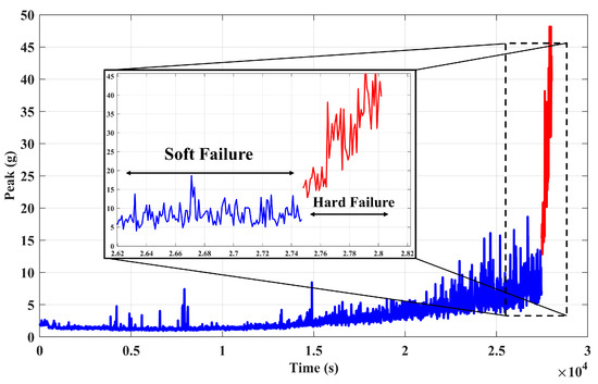
Figure 1.
Soft failure and hard failure stages in a run-to-failure test [9].
Guidelines highly recommended terminating the operation of a machine when its vibration level passes a specific limit. Manufacturers and some standard codes [3] suggest values for this limit based on the type and properties of the machines. This limit is employed to define a high-risk zone for the equipment. Moreover, the transformation of degradation from soft failure to hard failure corresponds to the changing vibrations from the stable stage to the unstable stage. The beginning the unstable stage can be interpreted as entering the high-risk zone. Therefore, if one can predict this transition point (from soft failure to hard failure), it can be used as the FT and define the end of life for the machine. Furthermore, instead of considering a static FT, predicting a probability distribution of the FT can enhance the reliability estimation.
There is no accurate and unanimous definition for the physical point of failure for a machine. Therefore, the recommendations of experts in the relevant field can be helpful in considering a limit for the high-risk region and decreasing failure possibility. In this paper, it is proposed that the high fluctuation occurrence in the vibration trend can be used as the FT in order to prevent machine operation in the high-risk zone. High fluctuation is assumed here to be an amount of 2 dB or ±25% variation of the vibration feature.
As mentioned in Section 2.2, PC1, which was proportional to the defect growth, was used as the degradation indicator. To provide a new suggestion for the FT, the relationship between vibration features and PC1 must be studied. With this aim, a conditional probability distribution of the vibration feature given variable PC1 was obtained through a proper copula model.
The conditional probability distribution function, in which 95% of the data are scattered in the range of ±25% around the mode of distribution, was used as the indicator of the initiation of high fluctuation in the vibration trend in this study. In other words, this distribution, H (F | PC1 ), should satisfy the equation below:
In Equation (9), F is the vibration feature most highly correlated with PC1, which was described in the previous subsections. The parameter fm is the mode of H (F | PC1 ). Since H was assumed to correspond to high fluctuation initiation, it represents the FT probability distribution and fm is suggested as an FT.
The procedure proposed in this paper to estimate the FT of REBs is summarized in the flowchart depicted in Figure 2. First, different vibration features in the time and frequency domains were extracted from the run-to-failure history. These features were the inputs to the PCA algorithm that produced a feature as a degradation indicator (PC1). Afterward, the vibration feature most highly correlated with PC1 was selected. By using the copula models, a suitable joint probability distribution was fitted for the selected feature and PC1. Finally, the FT probability distribution was obtained based on the proposed criterion.
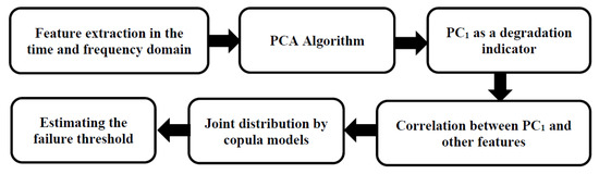
Figure 2.
Process of estimating the failure threshold (FT) for rolling element bearings (REBs).
3. Introducing Two Bearing Datasets
In this section, two experimental run-to-failure datasets are introduced to study the effectiveness of the method proposed in this paper. Dataset 1 corresponds to seven accelerated life tests of an REB in the laboratory. Dataset 2 corresponds to three run-to-failure tests of an REB in an industrial machine. The details of these two datasets will be introduced in the following subsections.
3.1. Dataset 1: Accelerated Life Test Dataset
A set of run-to-failure experiments were designed and conducted for the purpose of this research. The platform of these experiments is shown in Figure 3. Using this platform, an accelerometer was installed vertically on the housing of the test REB. The test REB was a 6907 deep groove single-row bearing (55 mm OD, 35 mm ID). The accelerated life experiments were conducted under constant operating conditions of 2000 rpm speed and 9000 N radial load. The sampling frequency for the accelerometer was 25.6 kHz. In these experiments, reaching an amplitude of 30 g in the acceleration signals was the test stop criterion.
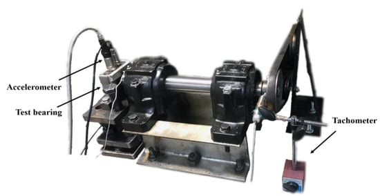
Figure 3.
The platform for the accelerated life experiments.
In total, seven run-to-failure experiments were conducted. Table 3 shows the final useful life results and the observed failure types in these experiments. At the end of the experiments, the observed failure in four tests related to the rolling elements and for the other three tests related to the inner race (Figure 4).
Table 3.
The useful life and the failure type of experiments.
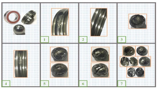
Figure 4.
The defects observed at the end of each accelerated life test.
3.2. Dataset 2: Industrial REB Dataset
As well as the accelerated life test dataset, the industrial data for a cylindrical roller bearing NU 2309 ECP (45 mm ID, 100 mm OD) of a sanding machine in a wood-based products manufacturing company was studied. These data were provided by Behravesh Vibration Engineering Company. The offline recorded vibration of this REB from March 2011 to June 2016 was provided for this research. In total, thirty-eight acceleration measurements in the frequency range of 10 to 8000 Hz were collected for this period. The trends for the RMS and the peak of the recorded signals in the mentioned period of time are depicted in Figure 5. During this period, three REB failures were detected and the machine was repaired. These three points are illustrated with a star (*) in the graph. These measurements were considered as three run-to-failure tests and their use in the study is described in the next section.
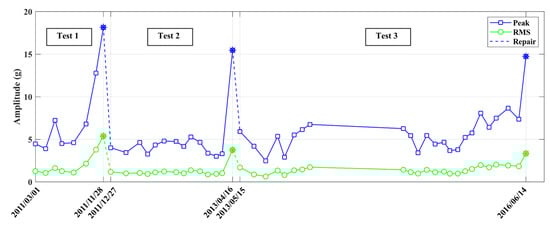
Figure 5.
The trends for the acceleration peak and root mean square (RMS) of an industrial REB.
4. Results
This section describes the application of the proposed method for FT determination to the two datasets introduced previously.
4.1. Calculating FT for Dataset 1 (Accelerated Life Test Dataset)
Three different scenarios were designed and considered in order to analyze the experimental data for this section. The results of the scenarios are presented as three models. In the first model, the features of all the data, without considering the failure modes, were given to the PCA algorithm to obtain the degradation indicator PC1. Then, a joint probability distribution was fitted between PC1 and the best correlated feature. With this distribution in hand, the approach proposed in Section 2.4 was applied to determine the FT. In the next two models, the experimental data were separated in order to be analyzed with regard to their occurred failure mode. In the second model, PC1 was extracted similarly to the previous model. However, data classified according to the failure mode was used to extract the joint probability distribution separately. Thus, considering separated joint distributions led to specific FTs for each failure mode. In the third model, a specific PC1 was extracted for each failure mode. Then, the FT was estimated similarly to the second model.
The reason for introducing the second and third models was to include consideration of the failure mode in the FT estimation. Model 1 did not include consideration of the failure mode at all. Model 2 included consideration of the failure mode only to generate the copula models. However, Model 3 considered the failure mode in the PCA algorithm as well as in the generation of the copula models.
4.1.1. Model 1: Proposing the FT without Considering the Failure Modes in PCA and Copulas
The time and frequency domain features (Table 1) were extracted from the run-to-failure test data. These features were given to the PCA algorithm as inputs and PC1 was calculated as the output of this algorithm. The five features most highly correlated with PC1 are specified in Table 4. It can be seen that the peak of the time signal had the highest correlation with PC1.
Table 4.
Correlation of time signal features with PC1. PCC, Pearson’s correlation coefficient.
Next, using the statistical copula models (described in Table 2), the Gumbel copula was selected as the best to create the joint probability distribution function. The criteria of the model fitness evaluation (RMSE and NSE) and corresponding parameter values are listed in Table 5. Thus, the Gumbel copula was employed to provide the joint probability distribution of the peak and PC1 (Figure 6).
Table 5.
Comparing the copula models’ goodness-of-fit parameters. RMSE, root mean square error; NSE, Nash–Sutcliffe efficiency.
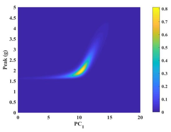
Figure 6.
Joint probability distribution between the peak and PC1 based on Gumbel copula.
Equation (6) can be used to obtain the conditional probability distribution function of the peak given PC1. According to the definition proposed for the FT in this paper, high vibration fluctuation occurred when PC1 was 13.5. The estimated distribution of the FT using the proposed method is represented in Figure 7. Moreover, the mode of distribution was 3.5 g. This value can be used as the constant value for the FT in predictions for the RUL problem.
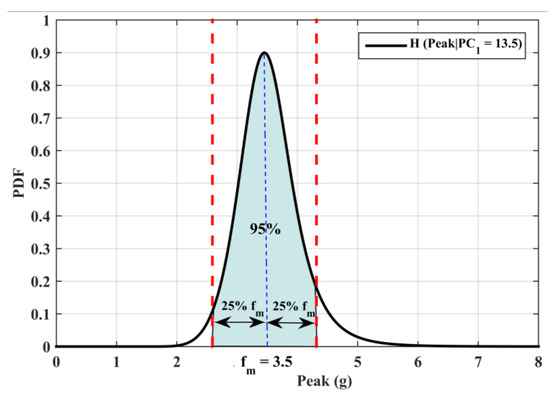
Figure 7.
Estimated FT distribution of model 1.
4.1.2. Model 2: Proposing the FT by Considering the Failure Modes in Copulas
In this model, PC1 was obtained using a similar approach to that described for the previous model. However, in the current model, the data classified by the failure modes were used to extract the joint probability distribution separately. Thus, having separated joint distributions resulted in a specific FT for each failure mode.
The experimental data used in this study were classified into two groups according to the observed failure mode (inner race failure or rolling element failure) at the end of each experiment (Table 3). Following the analysis of the correlation between vibration features with PC1, the peak of the time signal had the highest correlation for both failure modes (Table 6). Therefore, using the statistical copula models (Table 2), Gumbel and Gaussian copulas were chosen as the best to create the joint distribution functions for inner race and rolling element failure modes, respectively. The criteria of the model fitness evaluation and corresponding parameter values are listed inTable 7.
Table 6.
Correlation of time signal features with PC1 for two classes of experimental data.
Table 7.
Comparing the copula models’ goodness of fit parameters for each failure mode.
Finally, the conditional probability distribution function of the peak given PC1 was obtained using Equation (6). According to the definition of the FT proposed in this paper, the high fluctuation of vibration occurred for the rolling element degradation and inner race degradation when PC1 was equal to 15.1 and 35, respectively. Furthermore, the conditional distributions of the peak for the mentioned values of PC1 were extracted from the corresponding joint probability distributions. These distributions, which were used as the FT distributions, are depicted in Figure 8. Additionally, the mode of each distribution can be used as the FT value for the degradation of each component (3.1 g for the rolling element and 8.7 g for the inner race).
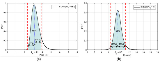
Figure 8.
Estimated FT distributions: (a) rolling element degradation (b) inner race degradation.
4.1.3. Model 3: Proposing the FT by Considering the Failure Modes in the PCA and Copulas
In this model, the classification of accelerated life tests was also considered in the PCA step. The data based on the rolling element or inner race failure modes were categorized and given to the PCA algorithm and PC1 was obtained for each failure mode separately. Then, considering the results of the correlation analysis displayed inTable 8, the peak feature for both failure modes was specified as the highest correlated feature. Comparisons of the goodness-of-fit parameters for different copulas are shown inTable 9. In light of the results shown in this table, the Gumbel copula was chosen as the best fitted copula model for both failure modes.
Table 8.
Correlation of time signal features with PC1 for two classes of experimental data.
Table 9.
Comparing the copula models’ goodness-of-fit parameters for each failure mode.
Finally, by calculating the conditional probability distribution function of the peak given PC1, the FTs were specified for rolling element degradation and inner race degradation when PC1 was equal to 11.2 and 40, respectively. Similar to the results reported for model 2, the FT distributions for the degradation of each failure mode are depicted in Figure 9. The mode values of the FT distributions were 5 g and 14.5 g for the rolling element degradation and the inner race degradation, respectively. These values can be considered as constant FTs.
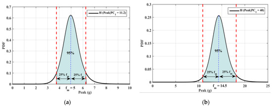
Figure 9.
Estimated FT distributions: (a) rolling element degradation (b) inner race degradation.
4.2. Calculating FT for Dataset 2 (Industrial REB Dataset)
In order to explore the significance of FTs in industrial applications, the approach presented in this study was applied to dataset 2. Since this dataset included limited sets of run-to-failure data (three sets in total), only model 1 was investigated. Furthermore, models 2 and 3 could not be employed since the failure modes were not clear in this dataset. As can be seen in Table 10, the peak of the time signal had the highest correlation with the PC1 resulting from the PCA algorithm. By comparing various copula families, the Gumbel copula was obtained as the most accurate one to model the joint probability distribution of data (Table 11).
Table 10.
Correlation of time signal features with PC1.
Table 11.
Comparing the copula models’ goodness-of-fit parameters.
The probability distribution of the FT was estimated through the aforementioned criterion (Figure 10). This distribution showed that the mode value of 10.5 g could be used as a proper FT value in this industrial REB.
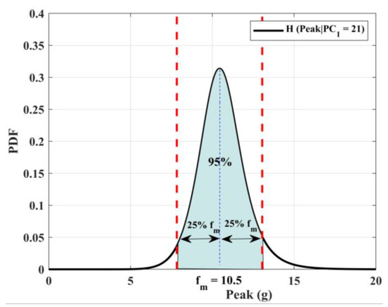
Figure 10.
Estimated FT distribution for dataset 2.
5. Discussion
5.1. Discussion on the Results of Dataset 1
As previously mentioned, the experimental accelerated life test data included seven run-to-failure tests, classified into two groups according to the type of final observed failure (Table 3). This subsection describes the application of the results of the FT estimation by the three models in Section 4.1 to these run-to-failure tests in order to compare their outputs.
The graphs in Figure 11 illustrate the trends for the vibration peak feature for three tests corresponding to inner race failure. In these graphs, three proposed values for the FT using the three models described in Section 4.1 are shown. The EoL estimation of each model is depicted by a star (*) on the trend. As can be seen, the estimated EoLs of the first and second models were close together and represent more conservative failure points than the third model. However, all of the models prevented unstable vibration. Also, the third model provided a more extended lifetime.
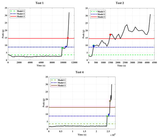
Figure 11.
Comparison of the FT models in the tests for inner race faults.
Similarly, the trends for the vibration peak in the four tests with the rolling element failure are shown in Figure 12. In this figure, it can be seen that the first and second models estimated the same EoL for all four tests. The third model also estimated a similar EoL in three tests out of four. However, in one test (test 7), the EoL estimated by model 3 was somewhat later than the two other models.
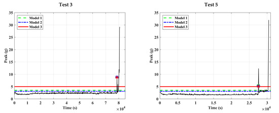
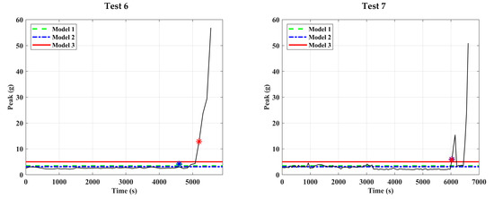
Figure 12.
Comparison of the FT models in the tests for rolling element faults.
The results of the three FT estimation models with regard to useful life for the seven tests are given in Table 12. The parameter ∆ is used to show the difference in useful life between the proposed models and the predetermined test stop criterion. The reader should note that this difference does not represent the error of the models presented in this paper since the predetermined criterion is just an assumption for stopping the tests and not the ideal.
Table 12.
The effect of FTs on REB useful life.
The highest value of ∆ was obtained in test 2. Comparing the vibration trends from all seven tests reveals the different behavior of the REB degradation in test 2. The vibration trend started to grow gradually from the beginning of its life. Furthermore, this REB had a relatively short life. The lack of a healthy stage in this test (unlike in the others) led to the high value of ∆.
Comparing the degradation trends for two groups of data shows that the degradation data included a soft failure stage when the growing defect was on the inner race. However, when the defect was on the rolling element, the soft failure stage did not exist. So, sudden growth and hard failure occurred after a healthy stage. The physical reason behind this behavior difference can be explained by the stress states in the rolling element and inner race. The smaller curvature radius in the rolling element (compared to the inner race) led to more severe stress and resulted in quicker degradation. Another explanation for this behavior could be the sharp edge flattening of spall regions that occurs in the inner race after removing particles from the surface. However, this flattening does not occur in the spall region of rolling elements [28].
In the third model proposed in this paper, the type of growing defect was considered in detail. Its output was therefore more accurate in estimating a proper EoL in the tests. However, model 1 proposed an EoL regardless of the type of failure and its output was more conservative than the others.
5.2. Discussion on the Results of Dataset 2
The peak trend for the industrial data on the three REB lifespans is depicted in a single plot in Figure 13. The total lifespans and the fluctuations of the vibrations in the three REBs can be compared in this figure. The FT extracted by analyzing these data with the approach proposed in this paper is depicted by a red dashed line in the figure.
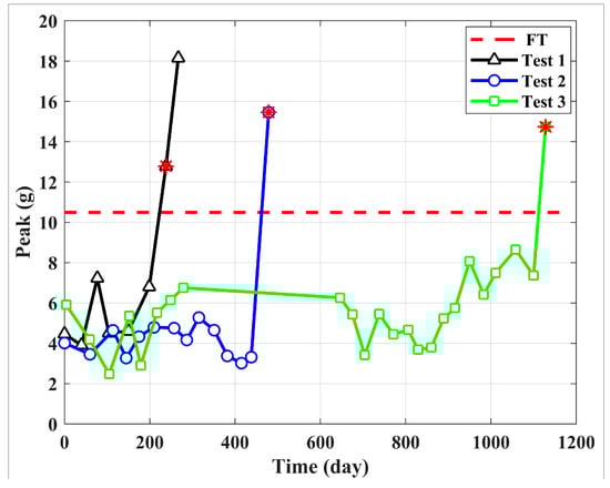
Figure 13.
Proposed FT for three tests of dataset 2.
Keeping in mind that there is no suggested FT for the acceleration of REBs in the guidelines, comparing the output of the proposed method with the actual decision of the condition monitoring (CM) group, which is based on their own experiences with the machine, shows that the proposed FT seems reasonable.
It should be noted that, since these data were gathered from an actual industrial field, the failure point in this dataset does not correspond to catastrophic failure and repairing activities were conducted to prevent such failure, based on CM recommendations. However, in the accelerated life tests which were previously discussed, the final failure referred to more severe and controlled damage under laboratory conditions.
In industrial applications, many of the machines are under the offline CM program. The available record during the degradation period is thus very limited. Since the goodness of fit in copula model estimation directly depends on the amount of available data, this limited data could affect the performance of the proposed algorithm.
6. Conclusions
In this paper, a method was suggested to determine the FT of REBs using vibration data. In this method, PCA was used to produce PC1 as a degradation growth indicator from vibration features. Moreover, copula models were applied to reveal the relationship between the vibration features and PC1. With the best-fitted copula model in hand, the FT distribution was defined as a probability distribution based on a 25% vibration fluctuation criterion and the mode of this distribution was used as a constant value for the FT. The proposed method was applied to one accelerated life test dataset as well as an industrial dataset. Applying the method to the accelerated life tests led to the development of three different models for the failure mode. The third model, which used the separated data of each failure mode for PCA and copula analysis, provided more accurate FTs that took the type of failure into account. It was shown that the estimated FT for the rolling element was less than that for the inner race. this was because of prompt growth of degradation after the initiation of the defect in the rolling element. Additionally, using model 1 to estimate the FT regardless of the failure mode led to a more conservative FT. Applying the method to the industrial data showed that the proposed method provided reasonable FTs for actual field data too. Due to the limitations of industrial data, only model 1 was used to estimate the FTs for this dataset.
FT selection plays a significant role in the RUL prediction of REBs. Since the method proposed in this paper estimates FTs using the high fluctuations in the degradation trend, it can provide a more accurate RUL prediction. Also, the provided FT distribution can be used in the reliability analysis of rotary machines. Furthermore, the method proposed in this paper can be used to estimate FTs under different machine operating conditions, which is what we plan to investigate in our future work.
Author Contributions
Conceptualization, S.F. and H.A.A.; investigation and methodology, S.F.; data curation, A.D.; writing—original draft preparation, S.F. and H.A.A.; writing—review and editing, M.B. and D.M.; visualization, S.F.; supervision, M.B.; All authors have read and agreed to the published version of the manuscript.
Funding
This research received no external funding.
Institutional Review Board Statement
Not applicable.
Informed Consent Statement
Not applicable.
Data Availability Statement
Data sharing not apllicable.
Acknowledgments
The authors gratefully thank Behravesh Vibration Engineering Co. and Takhte Feshorde Shomal Co. for their help in providing the industrial machine vibration condition monitoring data.
Conflicts of Interest
The authors declare no conflict of interest.
References
- Mahamad, A.K.; Saon, S.; Hiyama, T. Predicting remaining useful life of rotating machinery based artificial neural network. Comput. Math. Appl. 2010, 60, 1078–1087. [Google Scholar] [CrossRef]
- ISO. Standard ISO 13381-1. Condition Monitoring and Diagnostics of Machines—Prognostics—Part 1: General Guidelines; ISO: Geneva, Switzerland, 2015. [Google Scholar]
- ISO. Standard ISO 10816-3. Mechanical Vibration—Evaluation of Machine Vibration by Measurements on Non-Rotating Parts—Part 3: Industrial Machines with Normal Power above 15 kW and Nominal Speeds between 120 r/min and 15000 r/min; ISO: Geneva, Switzerland, 2009. [Google Scholar]
- Elasha, F.; Shanbr, S.; Li, X.; Mba, D. Prognosis of a wind turbine gearbox bearing using supervised machine learning. Sensors 2019, 19, 3092. [Google Scholar] [CrossRef] [PubMed]
- Wang, D.; Tsui, K.L. Two novel mixed effects models for prognostics of rolling element bearings. Mech. Syst. Signal Process. 2018, 99, 1–13. [Google Scholar] [CrossRef]
- Wang, Y.; Peng, Y.; Zi, Y.; Jin, X.; Tsui, K.L. A Two-Stage Data-Driven-Based Prognostic Approach for Bearing Degradation Problem. IEEE Trans. Ind. Inform. 2016, 12, 924–932. [Google Scholar] [CrossRef]
- Lim, C.K.R.; Mba, D. Switching Kalman filter for failure prognostic. Mech. Syst. Signal Process. 2015, 52, 426–435. [Google Scholar] [CrossRef]
- Bastami, A.R.; Aasi, A.; Arghand, H.A. Estimation of remaining useful life of rolling element bearings using wavelet packet decomposition and artificial neural network. IJSTE 2019, 43, 233–245. [Google Scholar] [CrossRef]
- Nectoux, P.; Gouriveau, R.; Medjaher, K.; Ramasso, E.; Chebel-Morello, B.; Zerhouni, N.; Varnier, C. PRONOSTIA: An experimental platform for bearings accelerated degradation tests. In Proceedings of the IEEE International Conference on Prognostics and Health Management, Denver, CO, USA, 18–21 June 2012; Available online: https://hal.archives-ouvertes.fr/hal-00719503 (accessed on 20 July 2012).
- Behzad, M.; Arghand, H.A.; Bastami, A.R. Remaining useful life prediction of ball-bearings based on high-frequency vibration features. Proc. Inst. Mech. Eng. Part C J. Mech. Eng. Sci. 2018, 232, 3224–3234. [Google Scholar] [CrossRef]
- Behzad, M.; Arghand, H.A.; Bastami, A.R. Rolling Element Bearings Prognostics Using High-Frequency Spectrum of Offline Vibration Condition Monitoring Data. In Proceedings of the Condition Monitoring and Diagnostic Engineering Management, Rustenburg, South Africa, 2–5 July 2018. [Google Scholar]
- Li, N.; Lei, Y.; Lin, J.; Ding, S.X. An improved exponential model for predicting remaining useful life of rolling element bearings. IEEE Trans. Ind. Electron. 2015, 62, 7762–7773. [Google Scholar] [CrossRef]
- Wang, P.; Coit, D.W. Reliability and degradation modeling with random or uncertain failure threshold. In Proceedings of the 2007 Annual Reliability and Maintainability Symposium, Orlando, FL, USA, 22–25 January 2007. [Google Scholar] [CrossRef]
- Nystad, B.H.; Gola, G.; Hulsund, J.E. Lifetime models for remaining useful life estimation with randomly distributed failure thresholds. In Proceedings of the First European Conference of the Prognostics and Health Management Society, 2012; Available online: https://www.phmsociety.org/node/788 (accessed on 30 May 2012).
- Yu, T.; Fuh, C.D. Estimation of Time to Hard Failure Distributions Using a Three-Stage Method. IEEE Trans. Reliab. 2010, 59, 405–412. [Google Scholar] [CrossRef]
- Qiu, H.; Lee, J.; Lin, J.; Yu, G. Wavelet Filter-based Weak Signature Detection Method and its Application on Roller Bearing Prognostics. J. Sound Vib. 2006, 289, 1066–1090. [Google Scholar] [CrossRef]
- Tobon-Mejia, D.A.; Medjaher, K.; Zerhouni, N.; Tripot, G. A Data-Driven Failure Prognostics Method Based on Mixture of Gaussians Hidden Markov Models. IEEE Trans. Reliab. 2012, 61, 491–503. [Google Scholar] [CrossRef]
- Cui, L.; Wang, X.; Xu, Y.; Jiang, H.; Zhou, J. A novel switching unscented Kalman filter method for remaining useful life prediction of rolling bearing. Measurement 2019, 135, 678–684. [Google Scholar] [CrossRef]
- Behzad, M.; Arghand, H.A.; Bastami, A.R.; Zuo, M.J. Prognostics of rolling element bearings with the combination of Paris law and reliability method. In Proceedings of the 2017 Prognostics and System Health Management Conference, Harbin, China, 9–12 July 2017. [Google Scholar] [CrossRef]
- Qian, Y.; Yan, R. Remaining useful life prediction of rolling bearings using an enhanced particle filter. IEEE Trans. Instrum. Meas. 2015, 64, 2696–2707. [Google Scholar] [CrossRef]
- Liu, Z.L.; Qu, J.; Zuo, M.J.; Xu, H. Fault level diagnosis for planetary gearboxes using hybrid kernel feature selection and kernel fisher discriminant analysis. Int. J. Adv. Manuf. Technol. 2013, 67, 1217–1230. [Google Scholar] [CrossRef]
- Nandi, A.K.; Ahmed, H. Condition Monitoring with Vibration Signals: Compressive Sampling and Learning Algorithms for Rotating Machines; John Wiley & Sons: Hoboken, NJ, USA, 2020. [Google Scholar]
- Malhi, A.; Gao, R.X. PCA-based feature selection scheme for machine defect classification. IEEE Trans. Instrum. Meas. 2004, 53, 1517–1525. [Google Scholar] [CrossRef]
- Sklar, M. Fonctions de repartition an dimensions et leurs marges. Publ. Inst. Statist. Univ. Paris. 1959, 8, 229–231. Available online: https://ci.nii.ac.jp/naid/10011938360/ (accessed on 21 July 2012).
- Sadegh, M.; Ragno, E.; AghaKouchak, A. Multivariate Copula Analysis Toolbox (MvCAT): Describing dependence and underlying uncertainty using a Bayesian framework. Water Resour. Res. 2017, 53, 5166–5183. [Google Scholar] [CrossRef]
- ISO. Standard ISO 15243, Rolling Bearings-Damage and Failures-Terms, Characteristic and Causes; ISO: Geneva, Switzerland, 2017. [Google Scholar]
- Harris, T.A.; Kotzalas, M.N. Advanced Concepts of Bearing Technology: Rolling Bearing Analysis; CRC Press: Boca Raton, FL, USA, 2006. [Google Scholar]
- Hoeprich, M.R. Rolling element bearing fatigue damage propagation. ASME. J. Tribo. 1992, 114, 328–333. [Google Scholar] [CrossRef]
Publisher’s Note: MDPI stays neutral with regard to jurisdictional claims in published maps and institutional affiliations. |
© 2020 by the authors. Licensee MDPI, Basel, Switzerland. This article is an open access article distributed under the terms and conditions of the Creative Commons Attribution (CC BY) license (http://creativecommons.org/licenses/by/4.0/).