Abstract
One of the important tasks in a graph is to compute the similarity between two nodes; link-based similarity measures (in short, similarity measures) are well-known and conventional techniques for this task that exploit the relations between nodes (i.e., links) in the graph. Graph embedding methods (in short, embedding methods) convert nodes in a graph into vectors in a low-dimensional space by preserving social relations among nodes in the original graph. Instead of applying a similarity measure to the graph to compute the similarity between nodes a and b, we can consider the proximity between corresponding vectors of a and b obtained by an embedding method as the similarity between a and b. Although embedding methods have been analyzed in a wide range of machine learning tasks such as link prediction and node classification, they are not investigated in terms of similarity computation of nodes. In this paper, we investigate both effectiveness and efficiency of embedding methods in the task of similarity computation of nodes by comparing them with those of similarity measures. To the best of our knowledge, this is the first work that examines the application of embedding methods in this special task. Based on the results of our extensive experiments with five well-known and publicly available datasets, we found the following observations for embedding methods: (1) with all datasets, they show less effectiveness than similarity measures except for one dataset, (2) they underperform similarity measures with all datasets in terms of efficiency except for one dataset, (3) they have more parameters than similarity measures, thereby leading to a time-consuming parameter tuning process, (4) increasing the number of dimensions does not necessarily improve their effectiveness in computing the similarity of nodes.
1. Introduction
Nowadays, graphs are becoming increasingly important since they are natural representations to encode relational structures in many domains (e.g., app’s function-call diagrams, brain-region functional activities, bio-medical drug molecules, protein interaction networks, citation networks, and social networks), where nodes represent the domain’s objects and links to their pairwise relationships [1,2,3,4,5,6,7]. Computing the similarity score between two nodes based on the graph structure is a fundamental task in a wide range of applications such as recommender systems, spam detection, graph clustering [8,9], web page ranking, citation analysis, social network analysis, k-nearest neighbor search [1,9], synonym expansion (i.e., search engine’s query rewriting and text simplification), and lexicon extraction (i.e., automatically building bilingual lexicons from text corpora) [10].
Link-based similarity measures (in short, similarity measures) such as SimRank [11] are well-known and conventional techniques to compute the similarity of nodes only based on the graph structure. Recently, SimRank and its variants have attracted a growing interest in the areas of data mining and information retrieval [1,8,9,10,12,13,14]. The philosophy of SimRank in similarity computation is that “two objects are similar if they are related to similar objects” [11]. In the literature, significant efforts have been devoted to improve the effectiveness of SimRank in similarity computation by proposing different variants such as SimRank++ [15], PSimRank [16], JacSim [1], JPRank [17], RoleSim [18], MatchSim [19], C-Rank [20], SimRank* [9], SimRank# [12], and PRank [21]. Among the aforementioned SimRank variants, JacSim, SimRank*, and JPRank are the state-of-the-art ones; JacSim solves the pairwise normalization problem [1,16,20], SimRank* solves the level-wise computation problem [9], and JPRank remedies both the pairwise normalization and in-links consideration problems [17,21] in the original SimRank. In addition, other variants such as GSimRank [14] and HowSim [8] have been proposed to compute the similarity of nodes in heterogeneous graphs where nodes have different types and links represent different types of relationships among nodes (However, in this paper, we only focus on the homogeneous graphs where nodes and links have a single type such as a citation graph where nodes represent papers and links to the citation relationship among them).
Graph embedding methods (in short, embedding methods), also known as feature representation learning methods, exploit the graph structure to represent each node in the graph as a low-dimensional vector in which neighborhood similarity, semantic information, and community structure among nodes in the graph are captured [22,23,24,25]. The obtained vector representations can be utilized by a wide range of tasks such as link prediction [22,24,26,27,28], node classification [22,23,25,26,27,28,29,30], recommendations [27], word analogy detection [25], and document classification [25]. Embedding methods, which are effective for extracting features from graph structured data, have broadly attracted significant attention in the literature and different embedding methods such as DeepWalk [23], Line [25], node2vec [26], graphGAN [27], NetMF [29], ATP [24], BoostNE [30], DWNS [22], and NERD [28] have been proposed for homogeneous graphs. In addition, some embedding methods have been proposed that target the heterogeneous graphs such as HeGAN [31], RTN [32], and HAN [33]. Some methods such as SIDE [34], CSNE [35], and nSNE [36] perform feature representation learning in signed graphs where there are two types of links (i.e., positive and negative) (In this paper, we focus only on the unsigned homogeneous graphs and the related embedding methods).
All of the aforementioned embedding methods encode the social relations among nodes into vectors in a continuous low-dimensional space where each dimension in this space can be interpreted as a latent feature [22,23,24,26]. In order to compute the similarity score of a pair of nodes in a given graph, we can apply Cosine [37] to their corresponding vector representations, similar to the strategy observed in the word analogy detection [25,38]. In other words, a link-based similarity measure computes the similarity between nodes by directly exploiting the graph structure, while an embedding method converts a node in the graph into a vector representation composed of a set of latent features by exploiting the graph structure, then these latent features preserving the graph structure properties can be used to compute the similarity between nodes.
Although a lot of efforts have been devoted to propose powerful embedding methods in the literature by analyzing them in a wide range of machine learning tasks, they are not comprehensively analyzed in terms of similarity computation of nodes in graphs. In this paper, we investigate and analyze both the effectiveness (i.e., accuracy) and efficiency (i.e., execution time) of embedding methods (i.e., DeepWalk, Line, node2vec, graphGAN, NetMF, ATP, BoostNE, DWNS, and NERD) in similarity computation of nodes and compare them with those of similarity measures (i.e., SimRank, JacSim, JPRank, and SimRank*). To the best of our knowledge, this is the first work that examines the application of embedding methods in computing the similarity of nodes. We conduct extensive experiments with five well-known and publicly available datasets as BlogCatalog [23,27,29], Cora [39,40], DBLP [1,17,41], TREC [1,17], and Wikipedia [26,27,29], which are widely used in the literature. Our experimental results demonstrate that similarity measures are better than embedding methods to compute the similarity of nodes; we found the following observations for embedding methods: (1) with all datasets, they show less effectiveness than similarity measures except for the BlogCatalog dataset; however, they show less efficiency than similarity measures with this dataset, (2) they underperform similarity measures with all datasets in terms of efficiency except for the Wikipedia dataset; however, with this dataset, they show less effectiveness than similarity measures, (3) they have more parameters than similarity measures, thereby leading to a difficult and time-consuming parameter tuning process, and (4) increasing the number of dimensions (i.e., latent features) does not necessarily improve their effectiveness in computing the similarity of nodes. In addition, we observe that, among embedding methods, DeepWalk and its variants (i.e., Line and NetMF) show better effectiveness.
The contributions of this paper are summarized as follows:
- Although embedding methods have been analyzed in a wide range of machine learning tasks, they are not investigated in terms of similarity computation of nodes. We investigate and analyze both the effectiveness and efficiency of embedding methods in the task of similarity computation of nodes in graphs.
- We compare the effectiveness as well as efficiency of embedding methods with those of link-based similarity measures as the conventional technique to compute the similarity of nodes.
- We conduct extensive experiments with five widely used datasets by employing nine different embedding methods and four different similarity measures, which all are state-of-the-art ones in the literature.
2. Link-Based Similarity Measures
In this section, we briefly explain SimRank [11], a well-known link-based similarity measure (in short, similarity measure), and its state-of-the-art variants as JacSim [1], JPRank [17], and SimRank* [9]; their corresponding mathematical formulations are represented in Appendix A.1, in detail.
SimRank: it computes the similarity between two nodes in a graph based on a philosophy that “two objects are similar if they are related to similar objects” [11]. For a node-pair in a graph, let and be two sets of nodes directly pointing to nodes a and b, respectively. In SimRank, the similarity score of is iteratively computed as the average of similarity scores of all possible node-pairs where node i belongs to and node j belongs to ; this computation manner is called a pairwise normalization paradigm [1]. Consider a sample graph in Figure 1; SimRank considers nodes e and f similar since they are directly pointed to by common node b (each node is highly similar to itself) and nodes i and j are regarded as similar since they are indirectly pointed to by common nodes c and d.
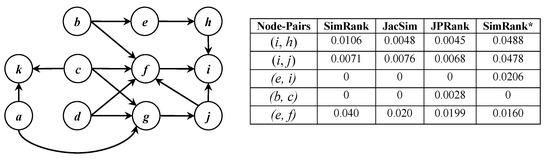
Figure 1.
A sample graph and similarity scores of some node-pairs.
JacSim: it tries to solve the pairwise normalization problem, by employing both Jaccard and pairwise normalization paradigm in similarity computation. This problem is a counter-intuitive property of SimRank where the SimRank score of a pair of nodes commonly pointed to by a large number of nodes tends to be lower than that of another pair of nodes commonly pointed to by a small number of nodes [1,16,20]. As an example, consider node-pairs and in the graph of Figure 1 where the similarity scores of some node-pairs are shown as well (We note that all the scores are computed by employing the matrix form of SimRank, JacSim, and JPRank); nodes i and h are pointed to by a single common node b, while nodes i and j are pointed to by two common nodes c and d. However, the SimRank score of (i.e., 0.0106) is bigger than that of (i.e., 0.0071) due to the pairwise normalization problem, while, as shown in the figure, the JacSim score of (i.e., 0.0048) is smaller than that of (i.e., 0.0076).
SimRank*: it is a variant of SimRank trying to remedy the level-wise computation problem in SimRank; this problem happens since SimRank regards two nodes similar if some paths only with equal length exist from a common node to both of them. As an example, consider the node-pair in Figure 1; there are no paths with the equal length from any common nodes such b to them. There is a path with length two from b to i, while there is a path with length one from b to e. Therefore, the SimRank score of becomes zero as shown in the figure due to the level-wise computation problem; however, their SimRank* score is not zero (i.e., 0.0206).
JPRank: it is another variant of SimRank that solves both the pairwise normalization and in-links consideration problems. The latter problem arises since SimRank considers only in-links to compute the similarity score. As an example, in Figure 1, the SimRank score of node-pair is zero since . However, both b and c are pointing to a common node f, which means b and c are somehow similar; as shown in the figure, the JPRank score of is not zero (i.e., 0.0028).
It is worth noting that, although our sample graph in Figure 1 is directed, all the above similarity measures can be applied to undirected graphs as well. However, the in-links consideration problem is not applicable to an undirected graph and JPRank behaves exactly the same as JacSim in similarity computation [17].
3. Graph Embedding Methods
In this section, we briefly describe the concept of graph embedding and explain some of the state-of-the-art graph embedding methods (in short, embedding methods) in the literature; their corresponding objective functions are represented in Appendix A.2, in detail.
For a given graph , graph embedding aims to learn a function that maps each node v in the graph into a vector in the d-dimensional space where [23,24,25,29]. The embedding methods exploit the graph structure to represent nodes as a low-dimensional vectors that encode the neighborhood similarity, semantic information, and community structure among nodes in the graph [22,23,24,25]. In the low-dimensional space, each dimension of the vectors can be interpreted as a latent feature [22,23,24,26]. Figure 2a illustrates the Zachary’s Karate graph [42] where the clusters found by modularity maximization are shown in different colors. We applied DeepWalk on this graph to obtain its two-dimensional representation, which is shown in Figure 2b; as an example, nodes 1 and 2 in the graph are represented as <−1.18, 1.15> and <−0.30, 1.10> vectors, respectively. As observed in the figure, there is a commonality between clusters in the original graph and its representation since they encode the social relations and community structure in the graph. Therefore, in order to compute the similarity score of node-pair in a given graph, we can calculate the proximity of the corresponding vector representations of a and b, similar to the strategy observed in the word analogy detection [25,38].
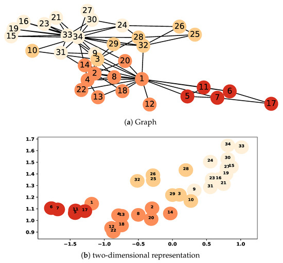
Figure 2.
Zachary’s Karate graph and its two-dimensional representation.
2
DeepWalk [23]: inspired by the remarkable achievements in the representation learning for natural language processing such as Skip-gram [38], it exploits a stream of short random walks to extract information from a graph where these short random walks can be regarded as a neighborhood for a target node consisting of n nodes before and after (i.e., window size ). DeepWalk tries to learn a model to maximize the probability of any node appearing in the ’s neighborhood without the knowledge of its offset from .
Line [25]: it considers the first-order proximity (i.e., direct neighbors of a node) and the second-order proximity to capture the nodes’ neighborhoods; the second-order proximity follows the sociology and linguistics theories where two nodes sharing similar neighbors tend to be similar. These proximities are preserved by utilizing two distinct objective functions where two different models for them are trained separately and their results are concatenated as the final result.
node2vec [26]: by following the homophily and structural equivalence hypotheses, it considers the community of a node and its structural roles in the graph, respectively, to capture the node neighborhood. node2vec utilizes a biased random walk controlled by two parameters p (return parameter) and q (in-out parameter). Suppose a random walk by using link in a graph; to decide the next walk from node v, parameter p controls the probability of revisiting previous node in the walk (i.e., u) and parameter q controls the probability of visiting a node close to v or visiting a node that is far from v.
graphGAN [27]: it considers two models, generator and discriminator , involving in a minimax game as follows. For a target node v, the generator tries to generate relevant nodes to the v’s neighborhood (i.e., found by BFS search rooted in v) and produces fabricated samples to deceive the discriminator, while the discriminator tries to detect whether a node actually belongs to v’s neighborhood or it is fabricated by the generator. In graphGAN, the objective is to train two models as a two-play minimax game.
NetMF [29]: it shows that graph embedding methods utilizing the Skip-gram model (e.g., DeepWalk, Line, and node2vec) with negative sampling perform implicit matrix factorization with a closed form. NetMF draws a theoretical connection between DeepWalk’s implicit matrix and graph Laplacians leading to constructing a low-rank connectivity matrix for DeepWalk, which is explicitly factorized by the singular value decomposition (SVD) technique [43] to obtain the representation vectors.
ATP [24]: it is a matrix-factorization-based embedding method that tries to preserve the asymmetric transitivity property in community question answering (CQA) graphs (i.e., if question is easier than and is easier than , then is easier than ). ATP constructs graph by removing cycle links from G, and incorporates both the graph reachability (i.e., transitive closure of [24]) and hierarchy (i.e., the rank of nodes in ) into a single matrix, which is factorized by a non-negative matrix factorization (NMF) technique [44] to obtain the representation vectors; each node has two corresponding vectors since its role in the graph is regarded as both a source and a target.
BoostNE [30]: it is a matrix-factorization-based embedding method that does not regard the low-rank assumption on the DeepWalk’s connectivity matrix M; applying a single NMF on M may lead to obtain such representations, which are insufficient to encode the connectivity patterns among nodes. Inspired by ensemble learning methods [45], BoostNE performs multiple levels of NMF on M to construct the representation vectors.
DWNS [22]: it applies the adversarial training method [46] to DeepWalk in order to improve the robustness and generalization ability of the learning process; it forces the learned classifier to be robust to adversarial examples (i.e., fabricated samples) generated from real ones through small perturbations. The training process is a two-player game where the adversarial samples are generated to maximize the model loss while the embedding vectors are optimized against them by utilizing stochastic gradient descent (SGD) [47].
NERD [28]: it mainly considers two different roles, a source and a target, for any nodes in the graph and maintains separate embedding spaces for the two distinct roles; based on this consideration, it exploits two distinct neighborhoods for each node and tries to maximize the likelihood of preserving both neighborhoods in their corresponding embedding spaces at the learning process.
4. Experimental Evaluation
In this section, we extensively analyze both the effectiveness (i.e., accuracy) and efficiency (i.e., execution time) of embedding methods (i.e., DeepWalk, Line, node2vec, graphGAN, NetMF, ATP, BoostNE, DWNS, and NERD) in the task of similarity computation of nodes in graphs with those of similarity measures (i.e., SimRank, JacSim, JPRank, and SimRank*) as the conventional technique for this task. Section 4.1 describes our experimental setup; Section 4.2 presents and analyzes the results.
4.1. Experimental Setup
All our experiments are performed on an Intel machine equipped with six 3.60 GHz i5-8600 CPUs, 64 GB RAM, and a 64-bit Fedora Core 31 operating system. All required codes are implemented with Python. We employ five well-known and publicly available datasets for our evaluation as follows. Table 1 shows some statistics of our datasets:

Table 1.
Some statistics about our datasets.
- BlogCatalog [23,27,29] is a graph representing social relationships among bloggers. The node labels denote blogger interests inferred through the metadata provided by the bloggers. This graph is fully tagged by 39 different labels.
- Cora [39,40] is a citation graph of academic papers in the area of computer science. The node labels denote the paper’s topic (e.g., Networking-Protocols). This graph is fully tagged by 70 different labels.
- DBLP [1,17,41] is a citation graph of academic papers in the areas of data mining and databases published in 2006 and earlier. The node labels denote the paper’s topic. This graph is partially tagged (i.e., 200 labeled nodes) by 11 different labels.
- TREC [1,17] is a hyperlink graph based on TREC 2003) (http://trec.nist.gov/data.html) where nodes represent web pages and links to the hyperlinks between web pages. The node labels denote the web page’s topic. This graph is partially tagged (i.e., 127 labeled nodes) by 11 different labels.
- Wikipedia [26,27,29] is a co-occurrence graph of words appearing in the first million bytes of the English Wikipedia dump. The labels represent the inferred Part-of-Speech (POS) tags of words. This graph is fully tagged by 40 different labels.
In the case of undirected graphs, we create two links in both directions. In order to evaluate the effectiveness (i.e., accuracy), we utilize MAP (mean average precision), precision, recall, F-score [37], and PRES [48] as evaluation metrics. In each dataset, we consider the labels as ground truth; for each label l, we use every single node with label l as a query node for a similarity based searching, and find those nodes that are considered similar to the query as a result set. If a node in the result set is labeled with l, it is regarded as relevant to the query, otherwise irrelevant. Then, we compute precision, recall, F-score, average precision (AP), and PRES for that query as follows:
where indicates the query result set, indicates the set of relevant nodes to the query (i.e., the set of all nodes labeled with l). and indicate the sizes of and , respectively. In the AP measure, a precision value is computed in each position (rank) in the query result set:
where indicates the precision at position k, is set as 1 if the node in position k is regarded as relevant. Otherwise, it is set as 0.
PRES considers the rank of retrieved relevant nodes in a result set and is computed as follows:
where is the rank of the relevant node in the result set; for each of those m (i.e., ) number of nodes that are relevant to the query but not retrieved in the result set, a rank is assigned by starting from the value of .
After computing the AP, precision, recall, F-score, and PRES for all the query nodes with label l, we take their average values to get MAP, precision, recall, F-score, and PRES values for label l. Then, we compute the average values of MAP, precision, recall, F-score, and PRES over all labels in the dataset. The aforementioned process is separately computed at top t (t = 5, 10, 20, 30) results; finally, the average accuracy over all values of t (e.g., we calculate the MAP value by taking the average of four MAP values at top 5, 10, 20, and 30 results) is regarded as the final accuracy for the dataset.
We implemented the matrix forms of SimRank, JacSim, JPRank, and SimRank* by applying the default parameter settings suggested by their original work with all datasets. We set the impact factor C as 0.8 for all four measures. For JacSim, the importance factor is set as 0.4 by following [1]. For JPRank, both importance factors and are set as 0.4 by following [17]; however, to indicate the value of weighting parameter , we conducted a very simple and fast experiment by following [17] to find out between in-links and out-links which one is more beneficial to similarity computation as follows. With each dataset, we computed SimRank based on in-links and out-links only on four iterations and then compared the accuracy of these two computations; is set as 0.9 if the similarity computation based on in-links shows better accuracy (i.e., with the DBLP dataset); it is set as 0.1, otherwise (i.e., with the TREC and Cora datasets (As explained in Section 2, JPRank behaves the same as JacSim with undirected graphs; we do not apply it to these graphs)).
In the case of embedding methods, we utilized the implementations with the default parameter settings provided by their original work (i.e., ATP (https://github.com/zhenv5/atp#atp-directed-graph-embedding-with-asymmetric-transitivity-preservation), BoostNE (https://github.com/benedekrozemberczki/BoostedFactorization), DeepWalk (https://github.com/phanein/deepwalk), DWNS (https://github.com/wonniu/AdvT4NE_WWW2019), graphGAN (https://github.com/hwwang55/GraphGAN), Line (https://github.com/tangjianpku/LINE), NERD (https://git.l3s.uni-hannover.de/khosla/nerd), NetMF (https://github.com/xptree/NetMF), and node2vec (https://github.com/aditya-grover/node2vec)). For ATP, we applied the H-voting technique (https://github.com/zhenv5/breaking_cycles_in_noisy_hierarchies) (it is not provided by the original implementation of ATP) to the datasets to find their cycle links. We could not apply graphGAN to Cora and TREC datasets since graphGAN requires lots of memory, and it does not run with these datasets on a machine with 64 GB memory. In order to compute the similarity between low-dimensional vectors, we implemented Cosine based on a matrix/vector multiplication technique, which is significantly faster than its conventional implementation. We made publicly available our implementations of the four similarity measures and Cosine along with the five aforementioned datasets here (https://github.com/mrhhyu/EMB_vs_LB).
4.2. Results and Analyses
In Section 4.2.1, for each dataset, we find the best iterations on which similarity measures show their highest accuracies. In Section 4.2.2, for each dataset, we find the best values of d (i.e., number of dimensions) for which the embedding methods show their highest accuracies in similarity computation of nodes. In Section 4.2.3 and Section 4.2.5, we present an experimental analysis on the effectiveness and efficiency of embedding methods (i.e., based on their best values of d) in comparison with similarity measures (i.e., based on their best iterations), respectively. Section 4.2.4 analyzes the impact of the value of d on the accuracy of embedding methods.
4.2.1. Link-Based Similarity Measures: Best Iterations
We apply the similarity measures to our five datasets on eight iterations; then, for each similarity measure with a dataset, we find out the best iteration on which the similarity measure shows its highest accuracy. Figure 3 illustrates the results with our five datasets; as an example, SimRank shows its highest accuracy on iterations 2 and 3 with the BlogCatalog and DBLP datasets, respectively. As already noted in Section 2, JPRank shows exactly the same results as JacSim does with undirected graphs; therefore, we do not apply JPRank to the BlogCatalog and Wikipedia datasets (i.e., 5 ∗ 4 − 2 = 18 experimental cases are conducted). In addition, in the figure, we do not represent the precision metric since the range of its values is higher than MAP, recall, PRES, and F-score; it makes the other four metrics plotted out very close together in the figure, thereby decreasing the readability of figures.
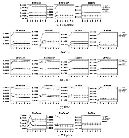
Figure 3.
Accuracy of similarity measures with all datasets on eight iterations.
As shown in Figure 3, for all similarity measures, the best iteration is observed before the eighth one in all datasets. Table 2 summarizes the best iterations for all similarity measures with our datasets. Note that, hereafter, when we compare the effectiveness of a similarity measure with those of embedding methods for a dataset, we consider the effectiveness of the similarity measure on its best iteration with that dataset; as an example, in the case of SimRank with the BlogCatalog dataset, we consider its effectiveness on the second iteration according to Table 2.
Table 2.
Best iterations of all similarity measures.
4.2.2. Graph Embedding Methods: Best Values of d
Now, we apply ATP, BoostNE, DeepWalk, DWNS, graphGAN, Line, NERD, NetMF, and node2vec to our five datasets to obtain the low-dimensional representation vectors of the nodes. Then, to compute the similarity between two nodes in a dataset, we apply Cosine to their corresponding vectors. In order to carefully analyze the impact of the number of dimensions d in similarity computation of nodes, we set d to different values as 64, 128, 256, and 512. For each possible combination of methods, datasets, and d values (e.g., ATP with the BlogCatalog dataset when ), we perform the experiment five times and select the best accuracy obtained among these five different executions as the final accuracy for that combination. More specifically, we conducted 900 () different experiments. Finally, similar to the strategy taken in Section 4.2.1, in the case of each embedding method with a dataset, we find out the best value of d for which the embedding method shows its highest accuracy in similarity computation of nodes.
Figure 4 and Figure 5 illustrate the accuracy of embedding methods with different values of d. The former figure shows the results with the BlogCatalog, Cora, and DBLP datasets, while the latter one shows the results with the TREC and Wikipedia datasets; as an example, BoostNE shows its highest accuracy when d is set as 256 and 128 with the BlogCatalog and TREC datasets, respectively. In these figures, we do not represent the precision metric due to the same reason as in Figure 3; the values of this metric with BlogCatalog, Cora, DBLP, TREC, and Wikipedia datasets for different values of d are represented in Table A1, Table A2, Table A3, Table A4 and Table A5 in Appendix A, respectively. As already noted in Section 4.1, we cannot apply graphGAN to the Cora and TREC datasets due to their large sizes. Table 3 summarizes the best value of d for all embedding methods with our datasets. Note that, hereafter, when we compare the effectiveness of embedding methods with those of similarity measures for a dataset, we consider the effectiveness of embedding methods on their best values of d with that dataset; as an example, in the case of DeepWalk with the BlogCatalog dataset, we consider its effectiveness based on according to Table 3.
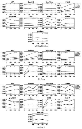
Figure 4.
Accuracy of embedding methods with BlogCatalog, Cora, and DBLP datasets for different values of d.
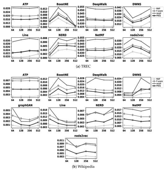
Figure 5.
Accuracy of embedding methods with TREC and Wikipedia datasets for different values of d.
Table 3.
Best values of d for all embedding methods.
4.2.3. Effectiveness Evaluation
In this section, we analyze the effectiveness (i.e., accuracy) of embedding methods in computing the similarity of nodes and compare it with those of similarity measures with each dataset as follows. As explained in Section 4.2.1 and Section 4.2.2, to compare the effectiveness of similarity measures with embedding methods for each dataset in this section, we consider their accuracies on their best iterations and best values of d represented in Table 2 and Table 3, receptively.
- BlogCatalog Dataset
Figure 6 illustrates the accuracy of all embedding methods and similarity measures with the BlogCatalog dataset. In this figure, we do not represent the precision measure due to the same reason as in Figure 3; instead, we show the precision values for all methods in Table 4. In addition, for those embedding methods and similarity measures that show comparable accuracies, we write down the values of their corresponding MAP, PRES, recall, and F-score in the figure to have better comparison.
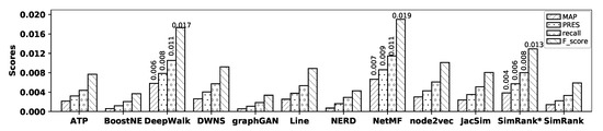
Figure 6.
Accuracy of embedding methods and similarity measures with the BlogCatalog dataset.
Table 4.
Precision values with the BlogCatalog dataset.
As observed in the figure, with the BlogCatalog dataset, NetMF shows the highest accuracy among all the embedding methods in terms of MAP, precision, recall, PRES, and F-score; however, its accuracy is close to that of DeepWalk, while BoostNE, graphGAN, and NERD show the worst accuracies. SimRank* shows better accuracy than other similarity measures, while SimRank shows the worst accuracy in terms of MAP, precision, recall, PRES, and F-score. Now, by comparing the accuracy of NetMF with that of SimRank*, it is observed that NetMF outperforms SimRank* by 73.44%, 35.68%, 42.89%, 50.00%, and 47.10% in terms of MAP, precision, recall, PRES, and F-score, respectively; Table 5 shows the percentage of improvements in accuracy obtained by NetMF over all other methods with the BlogCatalog dataset.
Table 5.
Accuracy improvements (%) by NetMF over other methods with the BlogCatalog dataset.
- Cora Dataset
Figure 7 illustrates the accuracy of all embedding methods and similarity measures with the Cora dataset and Table 6 shows the precision values for all methods.
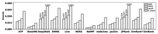
Figure 7.
Accuracy of embedding methods and similarity measures with the Cora dataset.
Table 6.
Precision values with the Cora dataset.
As observed in the figure, with the Cora dataset, although DeepWalk and Line show the best accuracy among all embedding methods, their accuracies are not tangible; Line outperforms DeepWalk in terms of recall, PRES, and F-score, while DeepWalk outperforms Line in terms of MAP and precision. NetMF and BoostNE show the worst accuracy among embedding methods in terms of all metrics. In the case of similarity measures, JPRank shows the best accuracy and SimRank again shows the worst one in terms of MAP, precision, recall, PRES, and F-score. Now, by comparing the accuracy of Line with that of JPRank, it is observed that JPRank slightly outperforms Line by 4.05%, 5.73%, 2.28%, 2.98%, and 3.05% in terms of MAP, precision, recall, PRES, and F-score, respectively; Table 7 shows the percentage of improvements in accuracy obtained by JPRank over all other methods with the Cora dataset.
Table 7.
Accuracy improvements (%) by JPRank over other methods with the Cora dataset.
- DBLP Dataset
Figure 8 illustrates the accuracy of all embedding methods and similarity measures with the DBLP dataset and Table 8 shows the precision values for all methods.
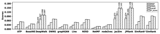
Figure 8.
Accuracy of embedding methods and similarity measures with the DBLP dataset.
Table 8.
Precision values with the DBLP dataset.
As observed in the figure, DeepWalk shows the best accuracy among all embedding methods, while NetMF shows the worst one in terms of MAP, precision, recall, PRES, and F-score. Among similarity measures, JPRank shows the best accuracy and it is close to that of JacSim, while SimRank shows the worst accuracy in terms of all metrics. Now, by comparing the accuracy of DeepWalk with that of JPRank, it is observed that JPRank outperforms DeepWalk by 64.89%, 50.34%, 51.70%, 52.71%, and 51.11% in terms of MAP, precision, recall, PRES, and F-score, respectively; Table 9 shows the percentage of improvements in accuracy obtained by JPRank over all other methods with the DBLP dataset.
Table 9.
Accuracy improvements (%) by JPRank over other methods with the DBLP dataset.
- TREC Dataset
Figure 9 illustrates the accuracy of all embedding methods and similarity measures with the TREC dataset and Table 10 shows the precision values for all methods.
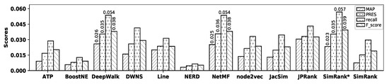
Figure 9.
Accuracy of embedding methods and similarity measures with the TREC dataset.
Table 10.
Precision values with the TREC dataset.
As observed in the figure, DeepWalk and NetMF show the best accuracy among all embedding methods in terms of MAP, precision, recall, PRES, and F-score. However, their accuracies are not tangible, where NetMF outperforms DeepWalk in terms of precision, PRES, and F-score, while DeepWalk shows better accuracy in terms of MAP and recall. NERD shows the worst accuracy among all embedding methods. SimRank* shows the best accuracy among all similarity measures, while SimRank shows the worst one in terms of all metrics. Now, by comparing the accuracy of NetMF with that of SimRank*, it is observed that they show very close accuracy; SimRank* outperforms NetMF in terms of precision, recall, and F-score, while NetMF outperforms SimRank* in terms of MAP and PRES. Table 11 shows the percentage of improvements in accuracy obtained by SimRank* over all other methods with the TREC dataset.
Table 11.
Accuracy improvements (%) by SimRank* over other methods with the TREC dataset.
- Wikipedia Dataset
Figure 10 illustrates the accuracy of all embedding methods and similarity measures with the Wikipedia dataset, and Table 12 shows the precision values for all methods. As observed in the figure, DeepWalk shows the highest accuracy among embedding methods in terms of MAP, precision, recall, PRES, and F-score; however, its accuracy is close to that of DWNS, while graphGAN shows the worst accuracy. Among similarity measures, JacSim shows the best accuracy, while SimRank shows the worst one in terms of all metrics. Now, by comparing the accuracy of DeepWalk with that of JacSim, it is observed that JacSim outperforms DeepWalk by 140.20%, 34.91%, 74.16%, 83.45%, and 66.55% in terms of MAP, precision, recall, PRES, and F-score; Table 13 shows the percentage of improvements in accuracy obtained by JacSim over all other methods with the Wikipedia dataset.
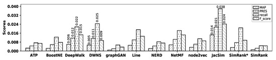
Figure 10.
Accuracy of embedding methods and similarity measures with the Wikipedia dataset.
Table 12.
Precision values with the Wikipedia dataset.
Table 13.
Accuracy improvements (%) by JacSim over other methods with the Wikipedia dataset.
4.2.4. Impact of d on Accuracy of Embedding Methods
In this section, we analyze whether increasing the number of dimensions improves the effectiveness of embedding methods in computing the similarity of nodes. In Section 4.2.2, Figure 4 illustrates the accuracy of all embedding methods with the BlogCatalog, Cora, and DBLP datasets for different values of d; in addition, Figure 5 illustrates the results of the same experiments with the TREC and Wikipedia datasets. As observed in these figures, in some cases such as DWNS and NetMF with the BlogCatalog dataset, increasing the number of dimensions improves the accuracy of the embedding methods (i.e., refer to Figure 4); on the contrary, in some cases such as Line with the Wikipedia dataset (i.e., refer to Figure 5) and graphGAN with the BlogCatalog dataset (i.e., refer to Figure 4), increasing the number of dimensions adversely affects the accuracy of the embedding methods. In addition, in some cases such as DeepWalk with the DBLP dataset (i.e., refer to Figure 4) and node2vec with the TREC dataset (i.e., refer to Figure 5), we observe both improvement and reduction in accuracy by increasing the number of dimensions. In summary, increasing the value of d does not help improve the accuracy of embedding methods in computing the similarity of nodes. In Section 4.2.2, Table 3 indicates the value of d showing the best accuracy for each embedding method with our datasets.
As represented in Table 3, some embedding methods show their best accuracies when or ; we call such a case a suspicious one since it may possible to improve the accuracy of the embedding method by assigning a lower (i.e., 32) or higher (i.e., 1024) value to d, respectively. However, if the accuracy of a suspicious case is not comparable with the accuracy of the best method in the dataset, conducting the aforementioned experiment is not beneficial since our overall observations will not be affected by the new result; for example, although ATP with the BlogCatalog dataset shows its highest accuracy when as a suspicious case, its accuracy is quite lower than that of NetMF as the best method for the same dataset (refer to Figure 6). In Table 3, there are only four following real suspicious cases that we need to consider them: both DeepWalk and Line show their highest accuracies when with the Cora dataset and their accuracies are very close to that of JPRank as the best method with Cora (i.e., refer to Figure 7). In addition, DeepWalk and NetMF show their highest accuracies when and with the TREC dataset, respectively; their accuracies are very close to that of SimRank* as the best method with TREC (i.e., refer to Figure 9). Therefore, we conduct the following four new experiments:
- DeepWalk with the Cora dataset and
- Line with the Cora dataset and
- DeepWalk with the TREC dataset and
- NetMF with the TREC dataset and
Table 14 represents the accuracies of the four new experiments (i.e., in bold face) along with the accuracies of their corresponding suspicious cases. In case 1, DeepWalk shows the same accuracy as it does when ; in addition, in cases 2 and 4, Line and NetMF show similar accuracies as they do when , respectively. In case 3, DeepWalk shows lower accuracy in comparison with . Therefore, we do not need to apply any changes in our results represented in Table 3.
Table 14.
Results of four extra experiments for suspicious cases.
4.2.5. Efficiency Evaluation
In this section, we carefully analyze the efficiency (i.e., execution time) of embedding methods in computing the similarity of nodes and compare it with that of similarity measures.
- Link-Based Similarity Measures
In order to conduct a fair comparison, we implemented the matrix form of JacSim, JPRank, SimRank*, and SimRank without applying any acceleration techniques such as multi-processing (as the simplest technique), fine-grained memorization [9], partial sums memoization [49], and backward local push and Monte Carlo sampling [50]. Since the execution time could slightly change depending on the system resources such as CPU overload, to obtain an accurate execution time, we run each similarity measure on eight iterations for five times with a dataset and the average run time over the five executions is regarded as the final execution time of the similarity measure. Note that we consider only the elapsed time to compute the similarity scores as the execution time; the required time to store the results of similarity computation in a file or a database is not considered.
Table 15 shows the execution time (minutes) of similarity measures with our five datasets (As already explained in Section 4.2.1, we do not apply JPRank to undirected graphs BlogCatalog and Wikipedia). With all datasets, SimRank* shows the best efficiency since it requires only one matrix multiplication in Equation (A8). With undirected datasets (i.e., BlogCatalog and Wikipedia), JacSim shows the worst efficiency since it requires two matrix multiplications and a pairwise normalization paradigm to compute matrix E in Equation (A6). With directed datasets (i.e., Cora, DBLP, and TREC), JPRank shows the worst efficiency since it requires four matrix multiplications and two pairwise normalization paradigms to compute matrices E and in Equation (A10). However, among all the available cases in Table 15, JacSim with the BlogCatalog dataset shows the worst efficiency, although BlogCatalog has less nodes than Cora, DBLP, and TREC datasets. The reason is that there are “32,787,165” node-pairs with non-empty common in-link sets in this dataset, which makes the calculation of matrix E expensive; the number of these node-pairs in Cora, DBLP, TREC, and Wikipedia datasets are “229,306”, “466,990”, “1,391,293”, and “11,015,803”, respectively.
Table 15.
Execution time (minutes) of all similarity measures with our datasets.
- Graph Embedding Methods
For embedding methods, the execution time is regarded as the summation of a learning time (i.e., elapsed time to construct low-dimensional representation vectors) and a similarity computation time (i.e., elapsed time to compute the similarity scores of all pairs of representation vectors by employing Cosine). With each dataset, the learning time of an embedding method is regarded as the average run time over the five executions of the method. We implemented Cosine based on a matrix/vector multiplication technique, which is significantly (i.e., almost 30 times) faster than its conventional implementation. In the case of similarity computation time, we consider only the elapsed time to compute the similarity scores by applying Cosine; the required time to store the results in a file or a database is not considered as we did for similarity measures.
Table 16 represents the learning time (minutes) of all embedding methods for different values of d with all datasets where bold face numbers indicate the best efficiency with each value of d in a dataset. As observed in the table, NetMF shows the best efficiency among all embedding methods with the BlogCatalog and Wikipedia datasets regardless of the value of d, node2vec shows the best efficiency among all methods with Cora, DBLP, and TREC datasets regardless of the value of d, BoostNE, and ATP almost have better efficiency after NetMF and node2vec with all datasets, and graphGAN shows the worst efficiency among all embedding methods with all datasets regardless of the value of d.
Table 16.
Learning time of all embedding methods for different values of d with all datasets.
Table 17 shows the similarity computation time (minutes) based on different vector sizes (i.e., ) with our five datasets. Note that the similarity computation time for a dataset depends on the number of node-pairs and the representation vector’s size (i.e., the value of d); for example, with the BlogCatalog dataset, the required time to compute Cosine for all node-pairs with vector size 64 obtained by any embedding methods (except APT and NERD) is 4.07. In the case of ATP and NERD with any value of d, the similarity computation time in Table 17 is multiplied by two since these methods construct two vectors for each node (i.e., target and source vectors) where we apply Cosine to the corresponding target vectors and source vectors of a node-pair separately; finally, the highest score is regarded as the final similarity score of the node-pair.
Table 17.
Similarity computation time (minutes) with different values of d for all datasets.
In order to easily compare the efficiency of all embedding methods at a glance, Figure 11 illustrates their execution times (i.e., the summation of the learning time and the similarity computation time) with all datasets; we excluded graphGAN since its execution time value is quite larger than other embedding methods. For example, with the BlogCatalog dataset when , the execution time of ATP is 11.83 as the summation of 3.69 (i.e., the learning time from Table 16) and (As explained before, for simplicity, we regard the similarity computation time as twice that in Table 17; for ATP with BlogCatalog when , the real Cosine calculation time is 8.33 (≃).) (i.e., twice the similarity computation time from Table 17); in addition, the execution time by DeepWalk is 45.32 as the summation of 41.25 (i.e., the learning time) and 4.07 (i.e., the similarity computation time).
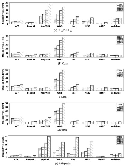
Figure 11.
Efficiency of embedding methods to compute the similarity of nodes with all datasets.
- Efficiency Comparison
In order to make a meaningful comparison, for each of our five datasets, we compare the efficiency of the best embedding method with that of the best similarity measure from Section 4.2.3, as follows:
- BlogCatalog: as observed in Figure 6, NetMF with (i.e., refer to Table 3) and SimRank* are the best embedding method and similarity measure showing highest accuracy, respectively. The execution time of NetMF with is 6.76 (i.e., 1.85 from Table 16 plus 4.91 from Table 17), while the execution time of SimRank* is 4.38 (refer to Table 15); SimRank* shows almost 35% better efficiency than NetMF.
- Cora: as observed in Figure 7, Line (i.e., with ) and JPRank are the best embedding method and similarity measure, respectively. The execution time of Line when is 60.31 (i.e., 34.62 + 25.69), while the execution time of JPRank with this dataset is 8.22; JPRank is almost 7.3 times more efficient than Line.
- DBLP: as observed in Figure 8, DeepWalk (i.e., with ) and JPRank show the highest accuracies among embedding methods and similarity measures, respectively. The execution time of DeepWalk when is 26.33 (i.e., 6.46 + 19.87) and that of JPRank is 8.41, which means that JPRank is 3.1 times more efficient than DeepWalk.
- TREC: as observed in Figure 9, NetMF with and SimRank* are the best embedding method and similarity measure, respectively. The execution time of the former method is 109.52 (i.e., 26.46 + 83.06) and that of the latter one is only 1.45, which means SimRank* is significantly faster than NetMF.
- Wikipedia: as observed in Figure 10, DeepWalk with and JacSim show the best accuracies among embedding methods and similarity measures, respectively. The execution time of DeepWalk when is 17.10 (i.e., 16.20 + 0.90) and the execution time of JacSim is 55.29, which means DeepWalk is almost 3.2 times faster than JacSim.
4.2.6. Discussion
Based on the results of our extensive experiments with embedding methods and similarity measures in Section 4.2.3 and Section 4.2.5, we observe that the latter technique is better than the former one to compute the similarity of nodes in graphs for the following reasons.
- First, similarity measures outperform embedding methods with all datasets in terms of effectiveness except with the BlogCatalog dataset where NetMF (i.e., with ) shows the better accuracy than SimRank*; however, its efficiency is 54% less than that of SimRank* with this dataset.
- Second, similarity measures show better efficiency with all datasets except with the Wikipedia dataset where DeepWalk (i.e., with ) is almost 3.2 times faster than JacSim; however, for this dataset, JacSim shows better effectiveness than DeepWalk and significantly outperforms it in terms of all five evaluation metrics as observed in Table 13.
- Third, similarity measures have a very low number of parameters than embedding methods, thereby leading to a simpler parameter tuning process to possibly obtain a better accuracy; for example, JPRank has only three parameters as , , and in Equation (A10), while DeepWalk has six parameters as the window size, walk length, number of dimensions, number of walks, size of training data, and learning tare.
In addition to the above findings, we observed that DeepWalk and its variants (i.e., Line and NetMF) show better effectiveness than other embedding methods in the task of similarity computation of nodes in graphs. Furthermore, it is shown that increasing the value of d (i.e., number of dimensions) does not help improve the accuracy of embedding methods in computing the similarity of nodes.
5. Conclusions
Embedding methods aim to represent each node in a given graph as a low-dimensional vector while preserving the neighborhood similarity, semantic information, and community structure of the nodes in the original graph. The dimensions in the low-dimensional vectors can be interpreted as latent features and the obtained vectors can be employed to compute the similarity of nodes in the graph. In this paper, we evaluated and compared both the effectiveness and efficiency of embedding methods in the task of computing similarity of nodes in graphs with those of link-based similarity measures by conducting extensive experiments with five datasets. We observed the following findings based on the results of our experiments. The similarity measures outperform embedding methods in terms of effectiveness with all datasets except with the BlogCatalog dataset where DeepWalk and NetMF show the best accuracy. The similarity measures are more efficient than embedding methods in similarity computation of nodes with all datasets except with the Wikipedia dataset where DeepWalk shows better efficiency. Finally, similarity measures are better to compute the similarity of nodes in graphs.
Author Contributions
Data curation, Formal analysis, Investigation, Software, Visualization, Writing—original draf, and Writing—review and editing, M.R.H.; Supervision, S.-W.K. All authors have read and agreed to the published version of the manuscript.
Funding
This research received no external funding.
Institutional Review Board Statement
Not applicable.
Informed Consent Statement
Not applicable.
Data Availability Statement
Publicly available datasets were analyzed in this study. This data can be found here: https://github.com/mrhhyu/EMB_vs_LB.
Acknowledgments
This work was supported by the National Research Foundation of Korea (NRF) grant funded by the Korea government (MSIT) (No. NRF-2020R1A2B5B03001960), the National Research Foundation of Korea (NRF) grant funded by the Korea government (MSIT) through the Life Basic Research Program (No. NRF-2019R1G1A1007598), and the Next-Generation Information Computing Development Program through the National Research Foundation of Korea (NRF) funded by the Ministry of Science, ICT (No. NRF-2017M3C4A7069440).
Conflicts of Interest
The authors declare no conflict of interest.
Appendix A
Appendix A.1
In this section, we present the mathematical formulation of SimRank, SimRank*, JacSim, and JPRank with their detailed description.
SimRank [11]: for a given graph where V represents a set of nodes and is a set of links among nodes, the SimRank score of a node-pair is defined as follows:
where is a set of nodes directly pointing to node a, is the size of , and is a damping factor. If or , . Equation (A1) is a recursive formula initialized by if ; , otherwise. For , we have
where on each iteration k, is computed based on similarity scores obtained in the previous iteration .
The iterative form of SimRank can be transformed to a closed matrix form [51,52], which is quite faster than the original iterative form. Let be a similarity matrix whose entry denotes ; then, SimRank scores are computed as follows:
where is a column normalized adjacency matrix whose entry if a points b; , otherwise. is a transpose matrix of Q, is an identity matrix, and term guarantees that the main diagonal entries in S are always maximum. The recursive computation of the matrix form starts with for , as follows:
JacSim [1]: it has both iterative and matrix forms; however, we explain its matrix form since it is more efficient than the iterative form while their accuracies are comparable [1]. Let be the similarity matrix; then,
where is an importance factor to control the degree of importance of Jaccard score and the one computed by the pairwise normalization paradigm, is a matrix whose entry denotes the Jaccard score of . is a matrix whose entry denotes the summation of JacSim scores of all node-pairs between and itself normalized by value . For , the recursive computation is started with as follows:
SimRank* [9]: let be the SimRank* similarity matrix; then,
where only one matrix multiplication is required since is a symmetric matrix and is identical to the transpose of . For , the recursive computation is started with as follows:
JPRank [17]: it has been proposed by both iterative and matrix forms; here, we explain its matrix form since it is more efficient than the iterative form while their accuracies are comparable [17]. Let be the JPRank similarity matrix; then,
where is a weighting parameter for in-links and out-links, and are used to control the degree of importance of the Jaccard score and the one computed by pairwise normalization paradigm based on in-links and out-links, respectively; is a row normalized adjacency matrix whose entry if a points b; , otherwise (i.e., is a set of nodes directly pointed to by node a). is a matrix containing the Jaccard score of node-pairs computed based on out-links. is a matrix whose entry denotes the summation of JPRank scores of all node-pairs in normalized by the values of . For , the recursive computation of JPRank is started with as follows:
Appendix A.2
DeepWalk [23]: it tries to learn a model by the following optimization function to maximize the probability of any node appearing in the ’s neighborhood with no knowledge of its offset from :
where the Skip-gram model equipped with a hierarchical softmax and the stochastic gradient descent (SGD) [47] are utilized to optimize the objective function.
Line [25]: first-order and second-order proximities are preserved by the two following objective functions, respectively:
where is the weight of the link between and (in unweighted graphs, it is set as one), is the vector representation of , and is the vector representation of when it is regarded as a neighbor in the second-order proximity of other nodes. Line employs a negative sampling technique based on the links’ weights and the asynchronous stochastic gradient descent (ASGD) [53]. Two models for the above objective functions are trained separately, and their results are concatenated as the final result.
node2vec [26]: it employs the following objective function:
where is a set of nodes as v’s neighborhood. The above objective function is optimized by utilizing the negative sampling and the stochastic gradient ascent.
graphGAN [27]: the objective is to train the two models as (tries to approximate the underlying true connectivity distribution of v, ) and (tries to discriminate the connectivity for the node-pair ) by the following two-play minimax game with a value function :
where and are the union of all vector representations of nodes u constructed by and , respectively. It employs a negative sampling technique where nodes truly connected to v are used as positive samples and some fabricated nodes are used as negative ones; is implemented by a softmax function, while is implemented by a graph softmax function [27].
NetMF [29]: it proposes the following low-rank connectivity matrix for DeepWalk:
where S denotes the volume of G (i.e., summation of all entries in A as the adjacency matrix of G), s is the number for negative samples, W is the window size, D is a diagonal matrix containing values of as its diagonal entries where is the degree of node , and P is defined as ; M is explicitly factorized by the singular value decomposition (SVD) technique [43] (i.e., ) where row i in matrix contains the representation vector of node .
ATP [24]: it incorporates the graph reachability and hierarchy through the following matrix M:
where and are constants, matrix contains the information of graph reachability (i.e., transitive closure of [24]), and diagonal matrix D keeps the information of the graph hierarchy in its diagonal entries (i.e., the value of is the rank of node i in ). Finally, a non-negative matrix factorization (NMF) technique [44] is applied to matrix M to generate a low-rank approximation of (i.e., and ) where row i and column i in matrices S and T contain the representation vectors of node when its role in the graph is regarded as a source and a target, respectively.
BoostNE [30]: it performs multiple levels of NMF resulting in the following objective function:
where k denotes the number of levels, contains the vector representations of nodes in level l, and contains the vector representations of nodes when they are treated as specific neighbors for other nodes in level l. For d (), the final matrix is obtained by assembling all partial representations where row i in is the representation vector of node .
DWNS [22]: the objective function is as follows:
where and denote the loss function of DeepWalk and the adversarial training regularizer, respectively. is a parameter to control the importance of the regularization term, denotes the model parameters, denotes the current model parameters, denotes the adversarial perturbation, denotes the adversarial noise level, and is the vector representation of node v.
NERD [28]: for two nodes u and v with roles and , respectively, NERD tries to find representations and by utilizing ASGD [53] to maximize the following objective function:
where denotes the sigmoid function, does the indegree (if is a target role) or outdegree (if is a source role) noise distribution, and s is the number of negative examples.
Appendix A.3
As explained in Section 4.2.2, we did not represent the precision metric in Figure 4 and Figure 5 since the range of its values is higher than MAP, recall, PRES, and F-score; it makes the other four metrics plotted out very close together in the figures, thereby decreasing the readability of figures. The values of this metric with BlogCatalog, Cora, DBLP, TREC, and Wikipedia datasets for different values of d are represented in the following tables, respectively.
Table A1.
Precision values of all embedding methods with the BlogCatalog dataset and different values of d.
Table A1.
Precision values of all embedding methods with the BlogCatalog dataset and different values of d.
| ATP | BoostNE | DeepWalk | DWNS | graphGAN | Line | NERD | NetMF | node2vec | |
|---|---|---|---|---|---|---|---|---|---|
| 0.083 | 0.039 | 0.161 | 0.070 | 0.047 | 0.105 | 0.037 | 0.155 | 0.117 | |
| 0.083 | 0.041 | 0.161 | 0.084 | 0.044 | 0.101 | 0.049 | 0.167 | 0.116 | |
| 0.084 | 0.045 | 0.156 | 0.096 | 0.039 | 0.101 | 0.048 | 0.17 | 0.115 | |
| 0.085 | 0.041 | 0.152 | 0.101 | 0.041 | 0.100 | 0.048 | 0.167 | 0.115 |
Table A2.
Precision values of all embedding methods with the Cora dataset and different values of d.
Table A2.
Precision values of all embedding methods with the Cora dataset and different values of d.
| ATP | BoostNE | DeepWalk | DWNS | Line | NERD | NetMF | node2vec | |
|---|---|---|---|---|---|---|---|---|
| 0.259 | 0.081 | 0.401 | 0.355 | 0.391 | 0.085 | 0.070 | 0.231 | |
| 0.302 | 0.105 | 0.401 | 0.367 | 0.391 | 0.283 | 0.075 | 0.231 | |
| 0.313 | 0.121 | 0.399 | 0.376 | 0.391 | 0.28 | 0.075 | 0.228 | |
| 0.325 | 0.129 | 0.398 | 0.376 | 0.391 | 0.28 | 0.075 | 0.224 |
Table A3.
Precision values of all embedding methods with the DBLP dataset and different values of d.
Table A3.
Precision values of all embedding methods with the DBLP dataset and different values of d.
| ATP | BoostNE | DeepWalk | DWNS | graphGAN | Line | NERD | NetMF | node2vec | |
|---|---|---|---|---|---|---|---|---|---|
| 0.046 | 0.024 | 0.107 | 0.074 | 0.036 | 0.050 | 0.013 | 0.019 | 0.036 | |
| 0.053 | 0.033 | 0.114 | 0.064 | 0.031 | 0.053 | 0.078 | 0.022 | 0.040 | |
| 0.057 | 0.028 | 0.107 | 0.081 | 0.029 | 0.052 | 0.072 | 0.021 | 0.039 | |
| 0.058 | 0.041 | 0.097 | 0.064 | 0.030 | 0.052 | 0.079 | 0.023 | 0.035 |
Table A4.
Precision values of all embedding methods with the TREC dataset and different values of d.
Table A4.
Precision values of all embedding methods with the TREC dataset and different values of d.
| ATP | BoostNE | DeepWalk | DWNS | Line | NERD | NetMF | node2vec | |
|---|---|---|---|---|---|---|---|---|
| 0.018 | 0.004 | 0.033 | 0.026 | 0.021 | 0.001 | 0.032 | 0.015 | |
| 0.017 | 0.008 | 0.033 | 0.015 | 0.021 | 0.005 | 0.033 | 0.021 | |
| 0.017 | 0.005 | 0.031 | 0.019 | 0.022 | 0.005 | 0.032 | 0.018 | |
| 0.018 | 0.001 | 0.032 | 0.025 | 0.022 | 0.005 | 0.034 | 0.012 |
Table A5.
Precision values of all embedding methods with the Wikipedia dataset and different values of d.
Table A5.
Precision values of all embedding methods with the Wikipedia dataset and different values of d.
| ATP | BoostNE | DeepWalk | DWNS | graphGAN | Line | NERD | NetMF | node2vec | |
|---|---|---|---|---|---|---|---|---|---|
| 0.041 | 0.04 | 0.056 | 0.041 | 0.035 | 0.06 | 0.045 | 0.056 | 0.052 | |
| 0.041 | 0.043 | 0.052 | 0.044 | 0.036 | 0.058 | 0.049 | 0.053 | 0.051 | |
| 0.041 | 0.043 | 0.05 | 0.046 | 0.034 | 0.056 | 0.048 | 0.05 | 0.051 | |
| 0.041 | 0.045 | 0.051 | 0.048 | 0.034 | 0.057 | 0.049 | 0.05 | 0.05 |
References
- Hamedani, M.R.; Kim, S.W. JacSim: An Accurate and Efficient Link-Based Similarity Measure In Graphs. Inf. Sci. 2017, 414, 203–224. [Google Scholar] [CrossRef]
- Ktena, S.I.; Parisot, S.; Ferrante, E.; Rajchl, M.; Lee, M.; Glocker, B.; Rueckert, D. Metric Learning with Spectral Graph Convolutions on Brain Connectivity Networks. NeuroImage 2018, 169, 431–442. [Google Scholar] [CrossRef] [PubMed]
- Li, Y.; Gu, C.; Dullien, T.; Vinyals, O.; Kohli, P. Graph Matching Networks for Learning the Similarity of Graph Structured Objects. In Proceedings of the 36th International Conference on Machine Learning (ICML), Long Beach, CA, USA, 9–15 June 2019; pp. 3835–3845. [Google Scholar]
- Wills, P.; Meyer, F.G. Metrics for Graph Comparison: A Practitioner’s Guide. PLoS ONE 2020, 15, 1–54. [Google Scholar] [CrossRef] [PubMed]
- Wu, Z.; Pan, S.; Chen, F.; Long, G.; Zhang, C.; Yu, P.S. A Comprehensive Survey on Graph Neural Networks. IEEE Trans. Neural Netw. Learn. Syst. (Early Access) 2020, 326. [Google Scholar] [CrossRef] [PubMed]
- Yoshida, T.; Takeuchi, I.; Karasuyama, M. Distance Metric Learning for Graph Structured Data. arXiv 2020, arXiv:2002.00727. [Google Scholar]
- Zhang, J. Graph Neural Distance Metric Learning with Graph-Bert. arXiv 2020, arXiv:2002.03427. [Google Scholar]
- Wang, Y.; Wang, Z.; Zhao, Z.; Li, Z.; Jian, X.; Xin, H.; Chen, L.; Song, J.; Chen, Z.; Zhao, M. Effective Similarity Search on Heterogeneous Networks: A Meta-path Free Approach. IEEE Trans. Knowl. Data Eng. (Early Access) 2020. [Google Scholar] [CrossRef]
- Yu, W.; Lin, X.; Zhang, W.; Pei, J.; McCann, J.A. Simrank*: Effective and Scalable Pairwise Similarity Search Based on Graph Topology. VLDB J. 2019, 28, 401–426. [Google Scholar] [CrossRef]
- Yu, W.; Wang, F. Fast Exact CoSimRank Search on Evolving and Static Graphs. In Proceedings of the 27th World Wide Web Conference (WWW), Lyon, France, 23–27 April 2018; pp. 599–608. [Google Scholar]
- Jeh, G.; Widom, J. SimRank: A Measure of Structural-Context Similarity. In Proceedings of the 8th ACM SIGKDD International Conference on Knowledge Discovery and Data Mining (KDD), Edmonton, AB, Canada, 23–26 July 2002; pp. 538–543. [Google Scholar]
- Yu, W.; McCann, J.A. High Quality Graph-Based Similarity Search. In Proceedings of the 38th International ACM SIGIR Conference on Research and Development in Information Retrieval (SIGIR), Santiago, Chile, 9–13 August 2015; pp. 83–92. [Google Scholar]
- Kusumoto, M.; Maehara, T.; ichi Kawarabayashi, K. Scalable Similarity Search for SimRank. In Proceedings of the 2014 International Conference on Management of Data (ACM SIGMOD), Snowbird, UT, USA, 22–27 June 2014; pp. 325–336. [Google Scholar]
- Zhang, C.; Hong, X.; Peng, Z. GSimRank: A General Similarity Measure on Heterogeneous Information Network. In Lecture Notes in Computer Science, Proceedings of Asia-Pacific Web and Web-Age Information Management Joint International Conference on Web and Big Data, APWeb-WAIM, Tianjin, China, 18–20 September 2020; Springer: Cham, Switzerland, 2020; pp. 588–602. [Google Scholar]
- Antonellis, I.; Molina, H.G.; Chang, C.C. Simrank++: Query Rewriting Through Link Analysis of the Click Graph. In Proceedings of the 17th International Conference on World Wide Web, Beijing, China, 21–25 April 2008; pp. 408–421. [Google Scholar]
- Fogaras, D.; Racz, B. Scaling Link-based Similarity Search. In Proceedings of the 14th International Conference on World Wide Web (WWW), Chiba, Japan, 10–14 May 2005; pp. 641–650. [Google Scholar]
- Hamedani, M.R.; Kim, S.W. Pairwise Normalization in Simrank Variants: Problem, Solution, and Evaluation. In Proceedings of the 34th ACM/SIGAPP Symposium on Applied Computing (ACM SAC), Limassol, Cyprus, 8–12 April 2019; pp. 534–541. [Google Scholar]
- Jin, R.; Lee, V.E.; Hong, H. Axiomatic Ranking of Network Role Similarity. In Proceedings of the 17th ACM SIGKDD International Conference on Knowledge Discovery and Data Mining (KDD), San Diego, CA, USA, 22–27 August 2011; pp. 922–930. [Google Scholar]
- Lin, Z.; Lyu, M.R.; King, I. Matchsim: A Novel Similarity Measure Based on Maximum Neighborhood Matching. Knowl. Inf. Syst. 2012, 32, 141–166. [Google Scholar] [CrossRef]
- Yoon, S.; Sang, S.W.K.; Sun-Ju, P. C-Rank: A Link-based Similarity Measure for Scientific Literature Databases. Inf. Sci. 2016, 326, 25–40. [Google Scholar] [CrossRef]
- Zhao, P.; Han, J.; Yizhou, S. P-Rank: A Comprehensive Structural Similarity Measure over Information Networks. In Proceedings of the 18th ACM Conference on Information and Knowledge Management (ACM CIKM), Hong Kong, China, 2–6 November 2009; pp. 553–562. [Google Scholar]
- Dai, Q.; Shen, X.; Zhang, L.; Li, Q.; Wang, D. Adversarial Training Methods for Network Embedding. In Proceedings of the 28th International Conference on World Wide Web (WWW), San Francisco, CA, USA, 13–17 May 2019; pp. 329–339. [Google Scholar]
- Perozzi, B.; Al-Rfou, R.; Skiena, S. DeepWalk: Online Learning of Social Representations. In Proceedings of the 20th ACM SIGKDD International Conference on Knowledge Discovery and Data Mining (KDD), New York, NY, USA, 24–27 August 2014; pp. 701–710. [Google Scholar]
- Sun, J.; Bandyopadhyay, B.; Bashizade, A.; Liang, J.; Sadayappan, P.; Parthasarathy, S. ATP: Directed Graph Embedding with Asymmetric Transitivity Preservation. In Proceedings of the 33rd AAAI Conference on Artificial Intelligence (AAAI), Honolulu, HI, USA, 27 January–1 February 2019; pp. 265–272. [Google Scholar]
- Tang, J.; Qu, M.; Wang, M.; Zhang, M.; Yan, J.; Mei, Q. LINE: Large-scale Information Network Embedding. In Proceedings of the 24th International Conference on World Wide Web (WWW), Florence, Italy, 18–22 May 2015; pp. 1067–1077. [Google Scholar]
- Grover, A.; Leskovec, J. node2vec: Scalable Feature Learning for Networks. In Proceedings of the 22nd ACM SIGKDD International Conference on Knowledge Discovery and Data Mining (KDD), San Francisco, CA, USA, 13–17 August 2016; pp. 855–864. [Google Scholar]
- Wang, H.; Wang, J.; Wang, J.; Zhao, M.; Zhang, W.; Zhang, F.; Xie, X.; Guo1, M. GraphGAN: Graph Representation Learning with Generative Adversarial Nets. In Proceedings of the 32nd AAAI Conference on Artificial Intelligence (AAAI), New York, NY, USA, 7–12 February 2018; pp. 2508–2515. [Google Scholar]
- Khosla, M.; Leonhardt, J.; Nejdl, W.; Anand, A. Node Representation Learning for Directed Graphs. In Lecture Notes in Computer Science, Proceedings of the European Conference on Machine Learning and Principles and Practice of Knowledge Discovery in Databases (ECML-PKDD), Würzburg, Germany, 16–20 September 2019; Springer: Cham, Switzerland, 2019; pp. 395–411. [Google Scholar]
- Qiu, J.; Dong, Y.; Ma, H.; Li, J.; Wang, K.; Tang, J. Network Embedding as Matrix Factorization: Unifying DeepWalk, LINE, PTE, and node2vec. In Proceedings of the 11st ACM International Conference on Web Search and Data Mining (WSDM), Marina Del Rey, CA, USA, 5–9 February 2018; pp. 459–467. [Google Scholar]
- Li, J.; Wu, L.; Guo, R.; Liu, C.; Liu, H. Multi-Level Network Embedding with Boosted Low-Rank Matrix Approximation. In Proceedings of the 2019 IEEE/ACM International Conference on Advances in Social Networks Analysis and Mining (ASONAM), Vancouver, BC, Canada, 25–29 August 2019; pp. 49–56. [Google Scholar]
- Hu, B.; Fang, Y.; Shi, C. Adversarial Learning on Heterogeneous Information Networks. In Proceedings of the 25th ACM SIGKDD International Conference on Knowledge Discovery and Data Mining (KDD), Anchorage, AK, USA, 25–29 August 2019; pp. 120–129. [Google Scholar]
- Gao, X.; Chen, J.; Zhan, Z.; Yang, S. Learning Heterogeneous Information Network Embeddings via Relational Triplet Network. Neurocomputing 2020, 412, 31–41. [Google Scholar] [CrossRef]
- Wang, X.; Ji, H.; Shi, C.; Wang, B.; Ye, Y.; Cui, P.; Yu, P.S. Heterogeneous Graph Attention Network. In Proceedings of the World Wide Web Conference (WWW), San Francisco, CA, USA, 13–17 May 2019; pp. 2022–2032. [Google Scholar]
- Kim, J.; Park, H.; Lee, J.E.; Kang, U. SIDE: Representation Learning in Signed Directed Networks. In Proceedings of the World Wide Web Conference (WWW), Lyon, France, 23–27 April 2018; pp. 509–518. [Google Scholar]
- Mara, A.; Mashayekhi, Y.; Lijffijt, J. CSNE: Conditional Signed Network Embedding. In Proceedings of the 29th ACM International Conference on Information and Knowledge Management (CIKM), New York, NY, USA, 19–23 October 2020; pp. 1105–1114. [Google Scholar]
- Song, W.; Wang, S.; Yang, B.; Lu, Y.; Zhao, X.; Liu, X. Learning Node and Edge Embeddings for Signed Networks. Neurocomputing 2018, 319, 42–54. [Google Scholar] [CrossRef]
- Manning, C.; Raghavan, P.; Schutze, H. Introduction to Information Retrieval; Cambridge University Press: Cambridge, UK, 2008. [Google Scholar]
- Mikolov, T.; Chen, K.; Corrado, G.; Dean, J. Efficient Estimation of Word Representations in Vector Space. arXiv 2013, arXiv:cs.CL/1301.3781. [Google Scholar]
- Ou, M.; Cui, P.; Pei, J.; Zhang, Z.; Zhu, W. Asymmetric Transitivity Preserving Graph Embedding. In Proceedings of the 22nd ACM SIGKDD International Conference on Knowledge Discovery and Data Mining (KDD), San Francisco, CA, USA, 22–27 August 2016; pp. 1105–1114. [Google Scholar]
- Šubelj, L.; Bajec, M. Model of Complex Networks Based on Citation Dynamics. In Proceedings of the 22nd International Conference on World Wide Web (WWW), Rio de Janeiro, Brazil, 13–17 May 2013; pp. 527–530. [Google Scholar]
- Hamedani, M.R.; Kim, S.W.; Kim, D.J. SimCC: A Novel Method to Consider both Content and Citations for Computing Similarity of Scientific Papers. Inf. Sci. 2016, 334–335, 273–292. [Google Scholar] [CrossRef]
- Zachary, W.W. An Information Flow Model for Conflict and Fission in Small Groups. J. Anthropol. Res. 1977, 33, 452–473. [Google Scholar] [CrossRef]
- Golub, G.H.; Loan, C.F.V. Matrix Computations, 4th ed.; Johns Hopkins University Press: Baltimore, MD, USA, 2013. [Google Scholar]
- Cheng, P.; Wang, S.; Ma, J.; Sun, J.; Xiong, H. Learning to Recommend Accurate and Diverse Items. In Proceedings of the 26th International Conference on World Wide Web (WWW), Perth, Australia, 3–7 April 2017; pp. 183–192. [Google Scholar]
- Suh, S.; Choo, J.; Lee, J.; Reddy, C.K. L-EnsNMF: Boosted Local Topic Discovery via Ensemble of Nonnegative Matrix Factorization. In Proceedings of the 16th IEEE International Conference on Data Mining (ICDM), Barcelona, Spain, 12–15 December 2016; pp. 479–488. [Google Scholar]
- Szegedy, C.; Zaremba, W.; Sutskever, I.; Bruna, J.; Erhan, D.; Goodfellow, I.; Fergus, R. Intriguing Properties of Neural Networks. arXiv 2014, arXiv:1312.6199. [Google Scholar]
- Bottou, L. Stochastic Gradient Learning in Neural Networks. In Proceedings of the Neuro-Nimes 91, Nimes, France, 4–8 November 1991. [Google Scholar]
- Magdy, W.; Jones, G.J. PRES: A Score Metric for Evaluating Recall-oriented Information Retrieval Applications. In Proceedings of the 33rd International Conference on Research and Development in Information Retrieval (ACM SIGIR), Geneva, Switzerland, 19–23 July 2010; pp. 611–618. [Google Scholar]
- Lizorkin, D.; Velikhov, P.; Grinev, M.; Turdakov, D. Accuracy Estimate and Optimization Techniques for SimRank Computation. In Proceedings of the VLDB Endowment, Auckland, New Zealand, 23–28 August 2008; pp. 422–433. [Google Scholar]
- Yu, W.; Zhang, W.; Lin, X.; Zhang, Q.; Le, J. Accelerating Pairwise SimRank Estimation Over Static and Dynamicgraphs. VLDB J. 2019, 28, 99–122. [Google Scholar]
- He, G.; Feng, H.; Li, C.; Chen, H. Parallel SimRank Computation on Large Graphs with Iterative Aggregation. In Proceedings of the 16th ACM SIGKDD International Conference on Knowledge Discovery and Data Mining (KDD), Washington, DC, USA, 24–28 July 2010; pp. 543–552. [Google Scholar]
- Yu, W.; Zhang, W.; Lin, X.; Zhang, Q.; Le, J. A Space and Time Efficient Algorithm for SimRank Computation. World Wide Web 2012, 15, 327–353. [Google Scholar] [CrossRef]
- Niu, F.; Recht, B.; Re, C.; Wright, S.J. HOGWILD!: A Lock-free Approach to Parallelizing Stochastic Gradient Descent. In Proceedings of the 24th International Conference on Neural Information Processing Systems (NIPS), Red Hook, NY, USA, 6–9 December 2010; pp. 693–701. [Google Scholar]
Publisher’s Note: MDPI stays neutral with regard to jurisdictional claims in published maps and institutional affiliations. |
© 2020 by the authors. Licensee MDPI, Basel, Switzerland. This article is an open access article distributed under the terms and conditions of the Creative Commons Attribution (CC BY) license (http://creativecommons.org/licenses/by/4.0/).