A Hierarchical Decision Fusion Diagnosis Method for Rolling Bearings

Abstract

In order to achieve accurate fault diagnosis of rolling bearings, a hierarchical decision fusion diagnosis method for rolling bearings is proposed. The hierarchical back propagation neural networks (BPNNs) architecture includes a fault detection layer, fault isolation layer and fault degree identification layer, which reduce the calculation cost and enhance the maintainability of the fault diagnosis algorithm. By wavelet packet decomposition and signal reconstruction of the raw vibration signal of a rolling bearing, the time-domain features of the reconstructed signals are extracted as the input of each BPNN and the accuracy of fault detection, fault isolation and degree estimation are improved. By using the majority voting method, the diagnosis results of multiple BPNNs are fused, which avoids the missed diagnosis and misdiagnosis caused by the insensitivity of a vibration characteristic to a specific fault. Finally, the proposed method is verified experimentally. The results show that the proposed method can accurately detect the fault of rolling bearings, recognize the fault location and estimate the fault severity under different operating conditions.

1. Introduction

The rolling bearing is one of the most frequently used parts in all kinds of mechanical equipment. About 30% of the faults in rotating machinery are caused by bearing faults, and the operating state of them will directly affect the machine’s performance [1,2]. Periodic load and impact are the main causes of rolling bearing wear, cracking, spalling and other failures [3]. Therefore, the importance of rolling bearing condition monitoring and fault diagnosis has been increasingly recognized and has drawn extensive attention in the past decades [4,5].

As the vibration signals contain abundant bearing state information, vibration-based methods have been widely used in the past few decades. Common vibration signal feature extraction methods include time-domain analysis [6], frequency domain analysis [7], time-frequency analysis [8,9] and other nonlinear analysis methods [10,11,12]. Conventional time-domain or frequency-domain methods have difficulty extracting minor fault information from rolling bearing vibration signals with background noise [13]. Therefore, the vibration signal processing methods came into being, such as sparse decomposition [14], empirical mode decomposition (EMD) [15], ensemble local mean decomposition (ELMD) [16], short time Fourier transform (STFT) [17], wavelet transform (WT) [18], wavelet packet transform (WPT) [19], spectral kurtosis (SK) [20], fast spectral kurtosis (FK) [21], etc. A number of cases have shown that wavelet packet decomposition combined with time-domain analysis is an effective feature extraction method [22]. However, time-domain features are diverse; thus, the selection of time-domain features has become the focus of research.

The traditional fault diagnosis method of rolling bearings is based on a classifier for pattern recognition of rolling bearings, while fault detection, isolation and degree estimation are realized [23,24,25]. However, this kind of method requires a large number of training samples and high representative features, which can easily lead to misdiagnosis. In order to reduce the risk of misdiagnosis caused by the complexity of the diagnosis system, Gan [26] proposed a hierarchical diagnosis network based on deep learning to identify the fault mode of rolling bearings using a two-layer diagnosis network. The fault location and fault degree were evaluated respectively. The results showed that the method has high reliability. However, most bearings are running in normal condition. The contingency of fault occurrence makes it very difficult to collect fault data and establish complete diagnosis knowledge, so the double-layer diagnosis network will face the problem of sample imbalance [27]. In addition, the key step of rolling bearing fault diagnosis is to extract the appropriate eigenvalue from the bearing signal as the diagnostic index and to realize the fault diagnosis of the rolling bearing by setting the threshold of the diagnostic index [28]. However, feature extraction and selection mainly depend on human experience, and fault diagnosis based on a single feature will be affected by external environmental factors or human factors and the result of classification will be unstable [29]. How to obtain fault diagnosis results with strong reliability and high stability and minimize the influence of sample imbalance on bearing fault diagnosis is one of the challenges of rolling bearing fault diagnosis.

Aiming at the above problems, a hierarchical back propagation neural networks (BPNNs) diagnosis method of rolling bearings based on decision fusion is proposed. The first layer is the fault detection decision fusion network, the second layer is the fault isolation decision fusion network and the third layer is the fault degree estimation decision fusion network. When the bearing is in normal condition, only the first layer is activated and the calculation cost is low, which overcomes the problems in the literature [26]. Hierarchical diagnosis architecture avoids the difficulty of neural networks training caused by incomplete raw data. In addition, when fault data is updated, only relevant neural networks need to be updated, which enhances the maintainability of the method. The wavelet packet decomposition and signal reconstruction of the raw vibration signals of the rolling bearing is carried out, and the time-domain characteristics of the reconstructed signals at each node are extracted as the input signal of the decision fusion networks, which improves the accuracy of the diagnostic results. The decision fusion networks model of each layer includes many BPNNs. A time-domain feature corresponds to a BPNN, and the diagnostic results of BPNNs are fused by the majority voting method. The highest diagnostic rate of the hierarchical diagnosis method can be obtained without artificial selection of time-domain features. Finally, the proposed method is verified experimentally. The results show that the proposed method can realize rolling bearing fault detection, fault location isolation and fault degree estimation under different operating conditions.

The structure of the paper is organized as follows: Section 2 introduces wavelet packet decomposition, BPNN and decision fusion based on the voting method, and proposes the rolling bearing hierarchical diagnosis method. Section 3 verifies the proposed method by experimental data. Section 4 provides the conclusion.

2. Method

2.1. Wavelet Packet Decomposition

Wavelet packet transform is an adaptive nonlinear analysis method, which can adaptively determine the resolution of different frequency bands and decompose the approximate part of the low frequency and the detailed part of the high frequency of the signal at the same time. Wavelet packet decomposition improves the time-frequency local analysis ability of the vibration signals, which can obtain higher time-domain resolution at high frequency and has higher frequency-domain resolution in the low-frequency part [30].

The scale function φ(x) and the wavelet function ψ(x) are represented by μ(x). The scale function on scale 0 is μ_0,0(x), and the scale function and wavelet function on scale 1 are μ_1,0(x) and μ_1,1(x).

$$\{\begin{array}{l}{\mu }_{1,0}(x)=\sqrt{2}{\displaystyle \sum _{k\in Z}{h}_k{\mu }_{0,0}(2x-k)}\\ {\mu }_{1,1}(x)=\sqrt{2}{\displaystyle \sum _{k\in Z}{g}_k{\mu }_{0,0}(2x-k)}\end{array}$$

(1)

For any scale j, the recursive equation of the function system ${\mu }_{j,m}(x)$ can be described as:

$$\{\begin{array}{l}{\mu }_{j,2m}(x)=\sqrt{2}{\displaystyle \sum _{k\in Z}{h}_k{\mu }_{j-1,m}(2x-k)}\\ {\mu }_{j,2m+1}(x)=\sqrt{2}{\displaystyle \sum _{k\in Z}{g}_k{\mu }_{j-1,m}(2x-k)}\end{array}$$

(2)

μ_j,m(x) is the orthogonal wavelet packet of the wavelet function ψ(x). As shown in Figure 1, a schematic diagram of n layer orthogonal wavelet packet decomposition for a signal is presented. The raw signal S is decomposed by a wavelet packet with n layers, and the signal at each node of each layer is decomposed into a low-frequency signal A and high-frequency signal D by the filter. The n layer wavelet packet decomposition will generate 2ⁿ nodes.

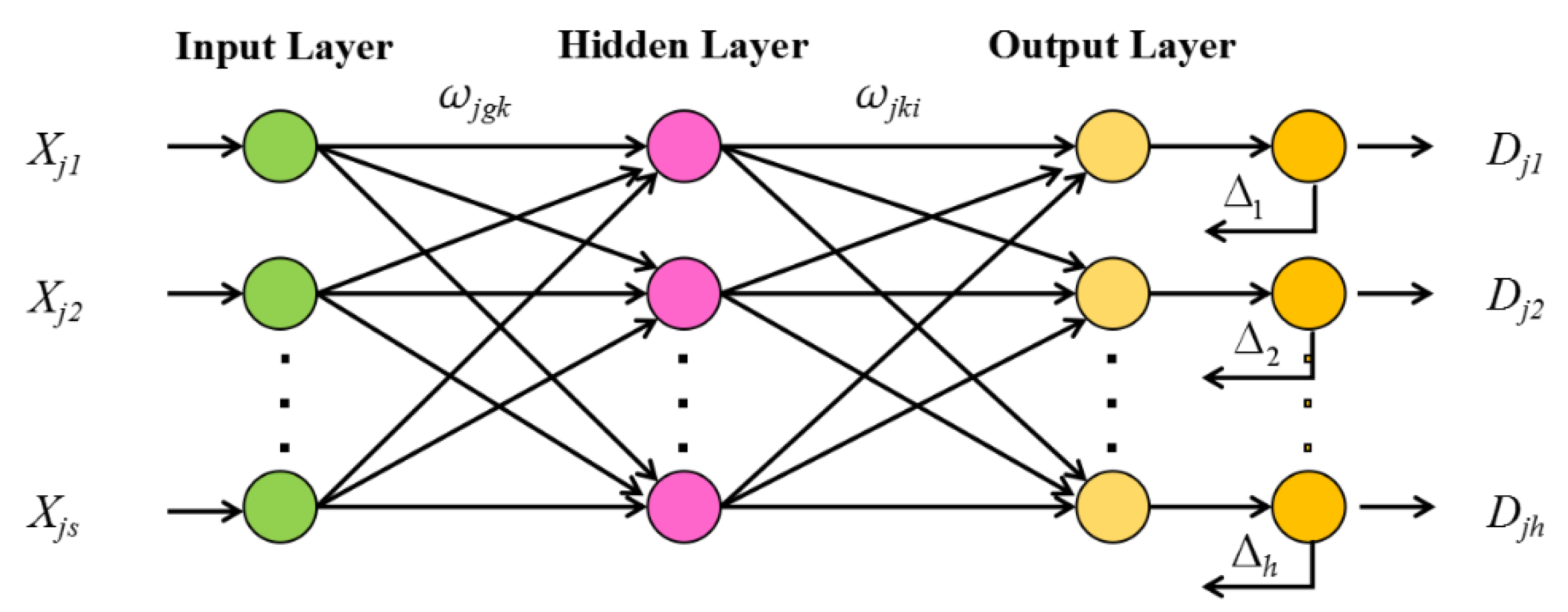
2.2. Back Propagation Neural Networks

The raw vibration signals are decomposed by a wavelet packet with n layers, producing s reconstructed signals. Features with the quantity of m are extracted from each reconstructed signal, forming the feature set F = {F₁, F₂, …, F_m}. F_j is normalized to X_j = {X_j1, X_j2, …, X_js}^T, which is the input of the jth BPNN. The number of output layer nodes is set to h, and the corresponding output is D_j = {D_j1, D_j2, …, D_jh}^T. The jth BPNN consists of an input layer, hidden layer and output layer, as shown in Figure 2.

In this paper, the training process of the jth BPNN consists of the following steps:

Step 1: Initialization.

The number of neurons in the hidden layer l is selected empirically. The weight ω_jgk connects the input layer with the hidden layer, and the weight ω_jki connects the hidden layer with the output layer. Then, the hidden layer threshold a_j and the output layer threshold b_j are initialized. The learning rate and neuronal excitation function are given in advance.

Step 2: Hidden layer calculation.

The output H_j of the hidden layer is calculated according to the input vector X, weight ω_jgk and hidden layer threshold a_j.

$$H_{jk}^{}=f\left({\displaystyle \sum _{g=1}^s{\omega }_{jgk}^{}{X}_{jg}^{}-a_{jk}^{}}\right), k=1,2,\dots ,l;j=1,2,\dots ,m$$

(3)

where f is the hidden layer excitation function. There are many excitation functions for the hidden layer, and the excitation function used in this paper is:

$$f(z)=\frac{1}{1+e^{-z}}$$

(4)

Step 3: The output calculation of the output layer.

The output of the jth BPNN D_j is calculated by the hidden layer output H_j, weight ω_jki and threshold b_j.

$$D_{ji}^{}={\displaystyle \sum _{k=1}^l{H}_{jk}^{}}{\omega }_{jki}^{}-b_{ji}^{},i=1,2,\dots ,h;j=1,2,\dots ,m$$

(5)

Step 4: Error calculation.

The network prediction error e_j is calculated based on the network prediction output D_j and the expected output Y_j.

e_ji = Y_ji − D_ji, i = 1, 2, …, h

(6)

Step 5: Weight update.

The network connection weights ω_jgk and ω_jki are updated by the network prediction error e_j.

$${\omega }_{jgk}^{}={\omega }_{jgk}^{}+\eta H_{jk}^{}(1-H_{jk}^{})X_{jg}^{}{\displaystyle \sum _{i=1}^h{\omega }_{jki}^{}{e}_{ji}^{},g=1,2,\dots ,s;k=1,2,\dots ,l;j=1,2,\dots ,m}$$

(7)

$${\omega }_{jki}^{}={\omega }_{jki}^{}+\eta H_{jk}^{}{e}_{ji}^{},k=1,2,\dots ,l;i=1,2,\dots ,h;j=1,2,\dots ,m$$

(8)

where $\eta$ is the learning ratio.

Step 6: Threshold update.

The network node threshold a_j and b_j are updated by the network prediction error e_j.

$$a_{jk}^{}=a_{jk}^{}+\eta H_{jk}^{}(1-H_{jk}^{}){\displaystyle \sum _{i=1}^h{\omega }_{jki}^{}{e}_{ji}^{},k=1,2,\dots ,l};j=1,2,\dots ,m$$

(9)

$$b_{ji}^{}=b_{ji}^{}+e_{ji}^{},i=1,2,\dots ,h;j=1,2,\dots ,m$$

(10)

Step 7: Iteration judgement.

Determining whether the algorithm iteration ends, and if not, returning to step 2.

A desired accuracy, $E_{Expect}$, is set. N is the sample number. If $\frac{1}{N}{\displaystyle \sum _{p=1}^N{\mathrm{e}}_j{}_p}>E_{Expect}$, a hidden neuron is added and the process returns to the second step; if $\frac{1}{N}{\displaystyle \sum _{p=1}^N{\mathrm{e}}_j{}_p}\le E_{Expect}$, the calculation is stopped.

2.3. Decision Fusion Based on the Voting Method

The idea of decision fusion comes from ensemble learning. Ensemble learning is not a single machine learning algorithm, but a method completing the task by building and combining multiple machine learning algorithms, which can be applied for classification problem integration, regression problem integration, feature selection integration, abnormal detection integration and so on [31,32]. For feature selection, Tripathi et al. [33] applied the data set with selected features to five base learners and aggregated the outputs obtained by the base classifier by a weighted voting method to predict the final output. A deep neural network algorithm, support vector machine (SVM) and decision tree c4.5 base classifiers were adopted by Asadi et al. [31], and the decision strategy based on the maximum number of votes was used to identify and classify botnets. Each ensemble learner produces a result, so it is necessary to integrate the results of each base learner to obtain the final decision result. A simple and effective way is to obtain the final decision result of multiple machine learning algorithms by the voting method. The voting method mainly includes the majority voting method [34] and the weighted voting method [33].

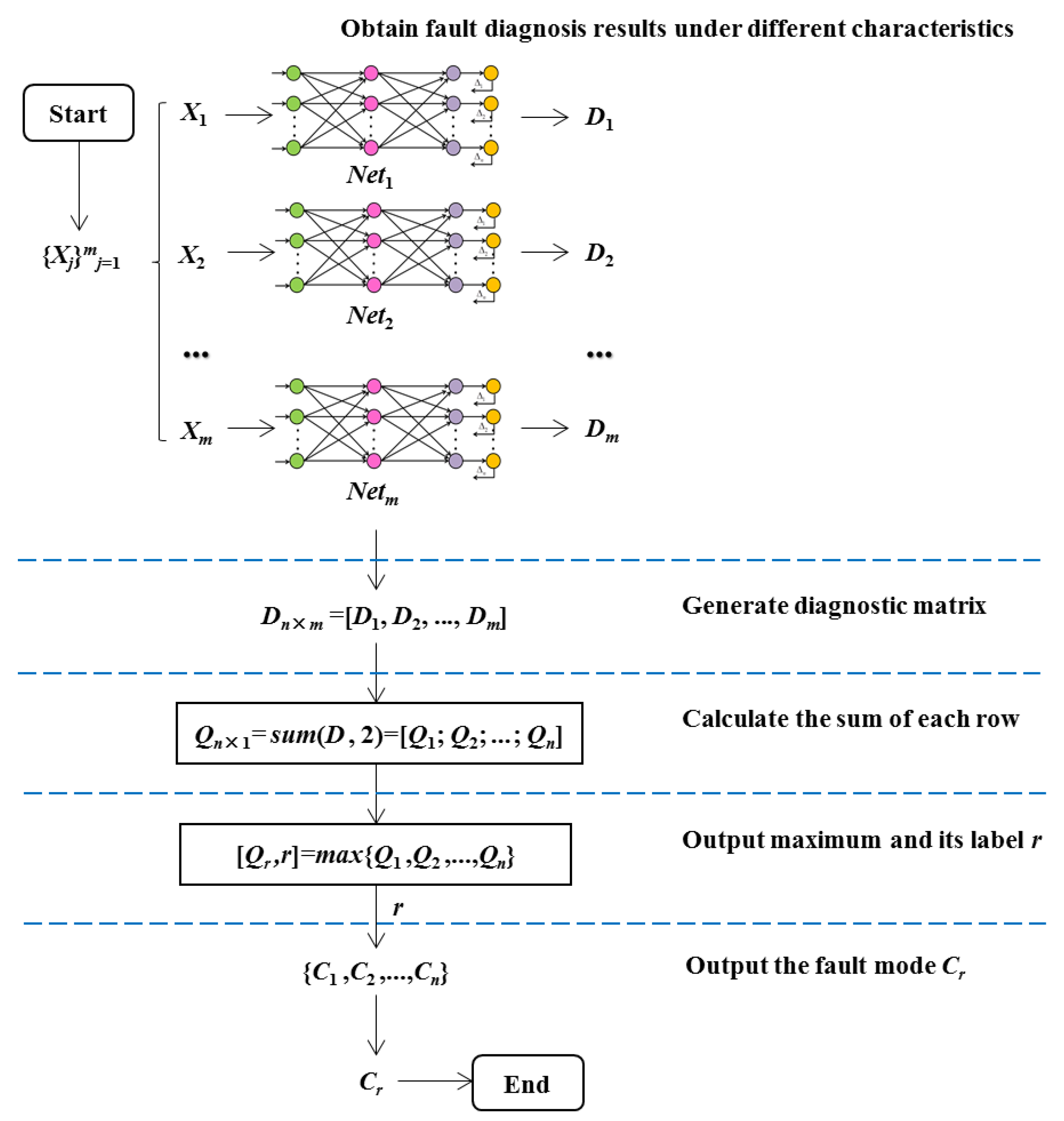
Inspired by the ensemble learning method, this paper makes use of the majority voting method to fuse the diagnosis results of multiple BPNN classifiers trained by a single feature set, which are extracted from all layers based on wavelet packet decomposition. Then, they are sorted from most to least. Finally, based on the principle that the minority obeys the majority, the diagnosis result with the largest number of votes is regarded as the decision fusion diagnosis result. The decision fusion algorithm based on the voting method is shown in Figure 3.

In Figure 3, m characteristics F₁, F₂, …, F_m are extracted from the vibration signals and are normalized to X₁, X₂, …, X_m as the input of m BPNN models Net₁, Net₂, …, Net_m, and then h kinds of fault modes of bearings are recognized, The output results D₁, D₂, …, D_m are Synthesized into a diagnostic matrix D_h×m. Then, each row of the matrix D_h×m is summed in order to get the scoring matrix Q_h×1 = {Q₁; Q₂; …; Q_h}. Each Q_i (i = 1, 2, …, h) represents the score of the fault mode i, respectively. Finally, the highest score Q_r is the output, which is the maximum of the output Q₁, Q₂, …, Q_h.

Setting fault discrimination matrix C:

{C₁; C₂; … ; C_h} = I_h×h

(11)

where C_i (i = 1, 2, …, h) represents the fault mode and I_h×h is an h-dimensional identity matrix. h is the total number of bearing state modes, which determines the number of output layer nodes.

The corresponding fault mode of the fault discrimination matrix C is found according to the angle mark r of the highest score, which is the decision fusion diagnosis result of the current state.

It can be seen that decision fusion is the fusion of multiple bearing fault diagnosis results based on a single time-domain feature. It is not necessary to screen the features, and the diagnostic results under each feature contribute to the final decision results. The decision fusion method takes into account the diagnostic advantages of each single time-domain feature for rolling bearing signals, and the diagnostic results based on the reasoning of each single time-domain feature will be comprehensively analyzed. To some extent, it can avoid the misdiagnosis and missed diagnosis of rolling bearing faults caused by the sudden change of environmental or human factors, which is helpful in reflecting the healthy condition of rolling bearings more comprehensively and accurately.

In addition, this paper adopts the winner-take-all strategy, which is suitable for single faults. For multi-fault cases, a feasible method is to sort according to the score of Q₁, Q₂, …, Q_h, from high to low, and output the order of the possibility of the fault mode, which can realize simultaneous fault diagnosis.

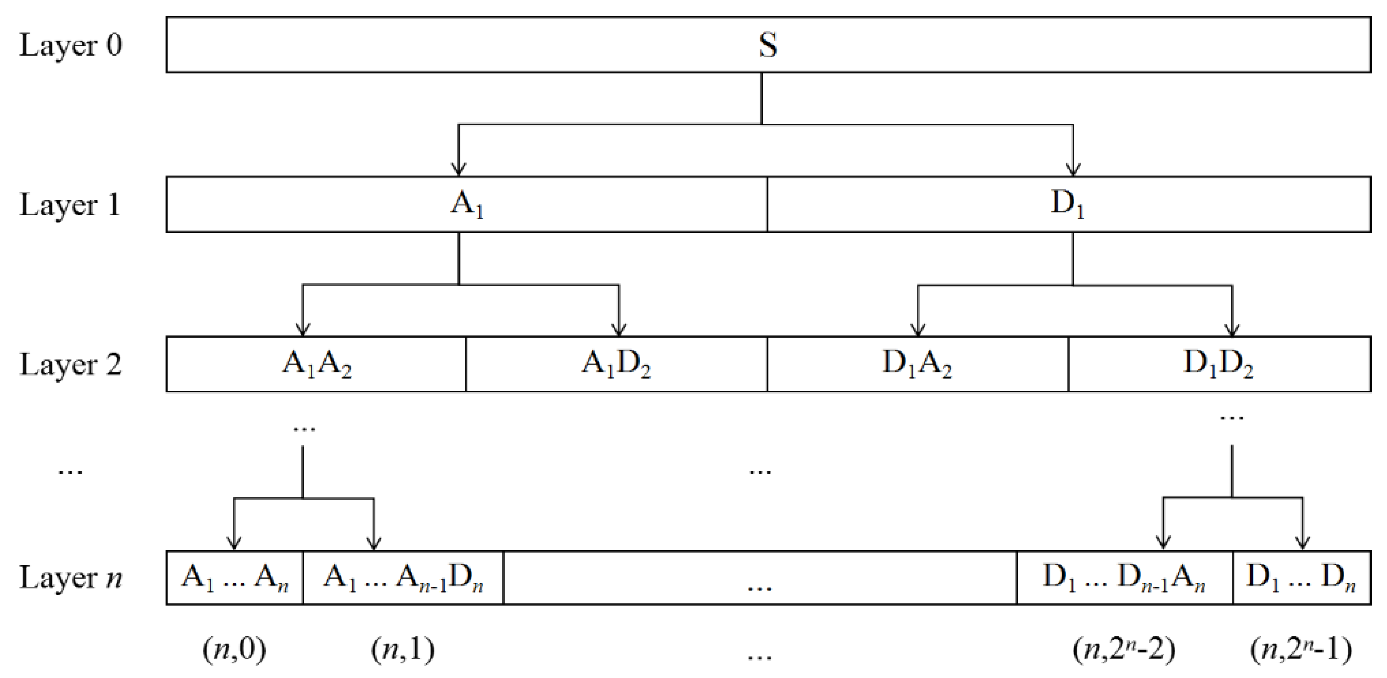
2.4. Hierarchical Fault Diagnosis Strategy

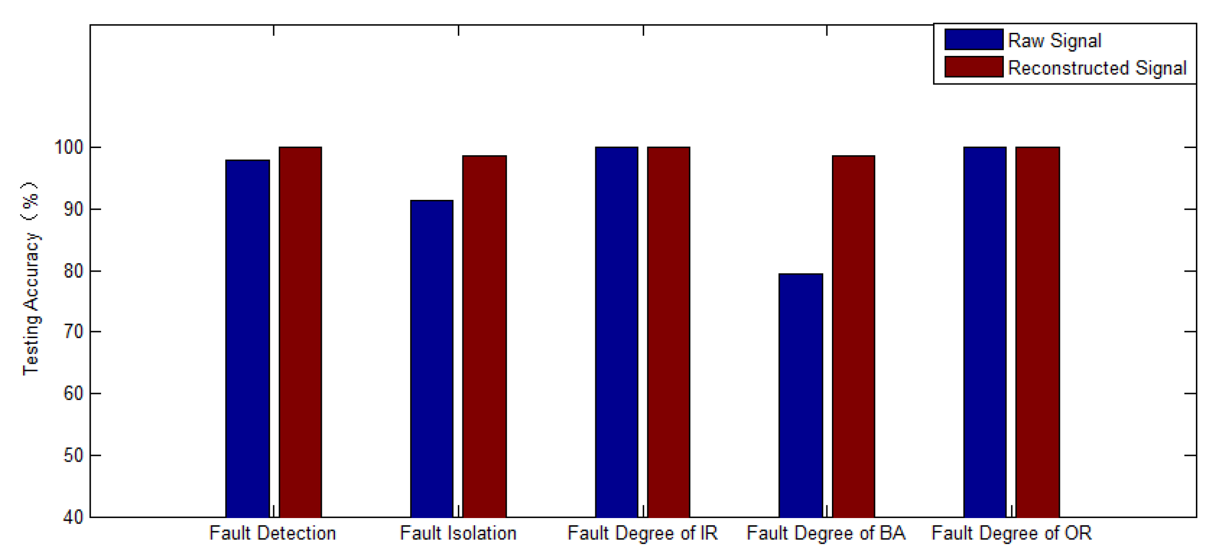
The traditional fault diagnosis method based on machine learning is to consider the fault position and severity synthetically. However, most of the rolling bearings are in normal condition, the fault occurs by chance and the evolution of the fault degree is nonlinear. In addition, in the actual process, the complete bearing fault samples are difficult to obtain. In this case, the fault diagnosis network that can judge the fault at the same time is often difficult to train because of the complexity of its network structure. In this paper, the hierarchical fault diagnosis architecture of rolling bearings is proposed, and the hierarchical diagnosis of rolling bearings is carried out in the progressive way. Further, the fault diagnosis of rolling bearings is divided into three layers: the first layer is the fault detection layer, which is used to judge whether the current state of the bearing is normal or not. The second layer is the fault isolation layer, and its goal is to identify the fault position of the bearing diagnosed as having a faulty state in the first layer. The third layer is the fault degree estimation layer, which is to further estimate the severity of the fault position of the rolling bearing.

The advantages of the hierarchical diagnosis proposed in this paper are as follows: the function of each layer of the neural network is relatively simple, the corresponding level of fault diagnosis network is trained by using the obtained fault samples, and the network training time is reduced. It is also relatively easy to improve the accuracy of fault identification. In addition, updating the fault algorithm is relatively easy, as it is only necessary to retrain the affected neural network to achieve the algorithm update, compared with the traditional diagnosis method; it also has better flexibility. Hierarchical decision fusion fault diagnosis methods include a training stage and a diagnosis stage.

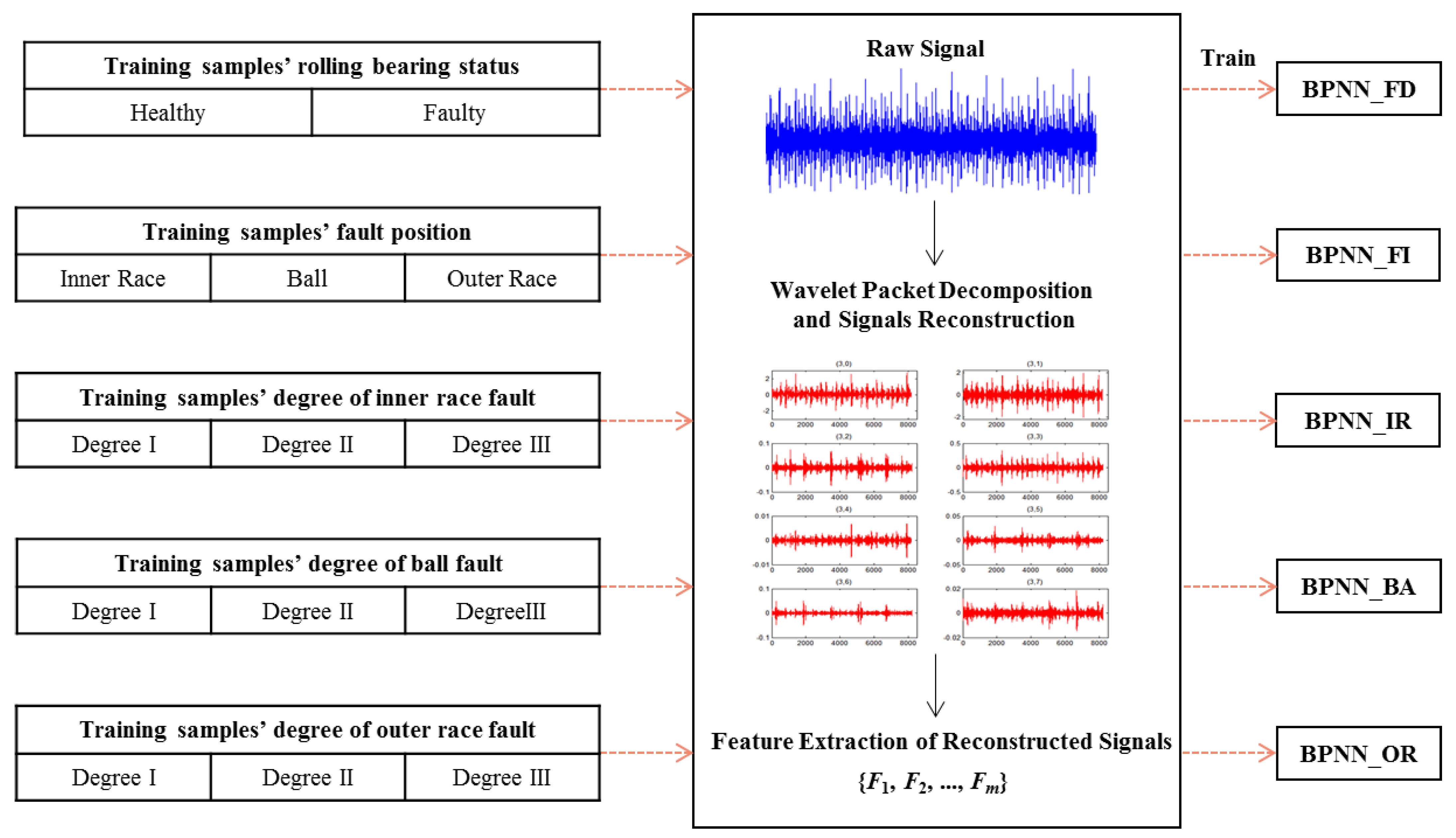
(1) Training Stage

The training stage of the hierarchical decision fusion fault diagnosis method is shown in Figure 4.

Step 1: Generate training samples.

According to the hierarchical fault diagnosis architecture, five kinds of training samples are designed, including a bearing state training sample, fault position training sample, inner race fault degree training sample, ball fault degree training sample and an outer race fault degree training sample.

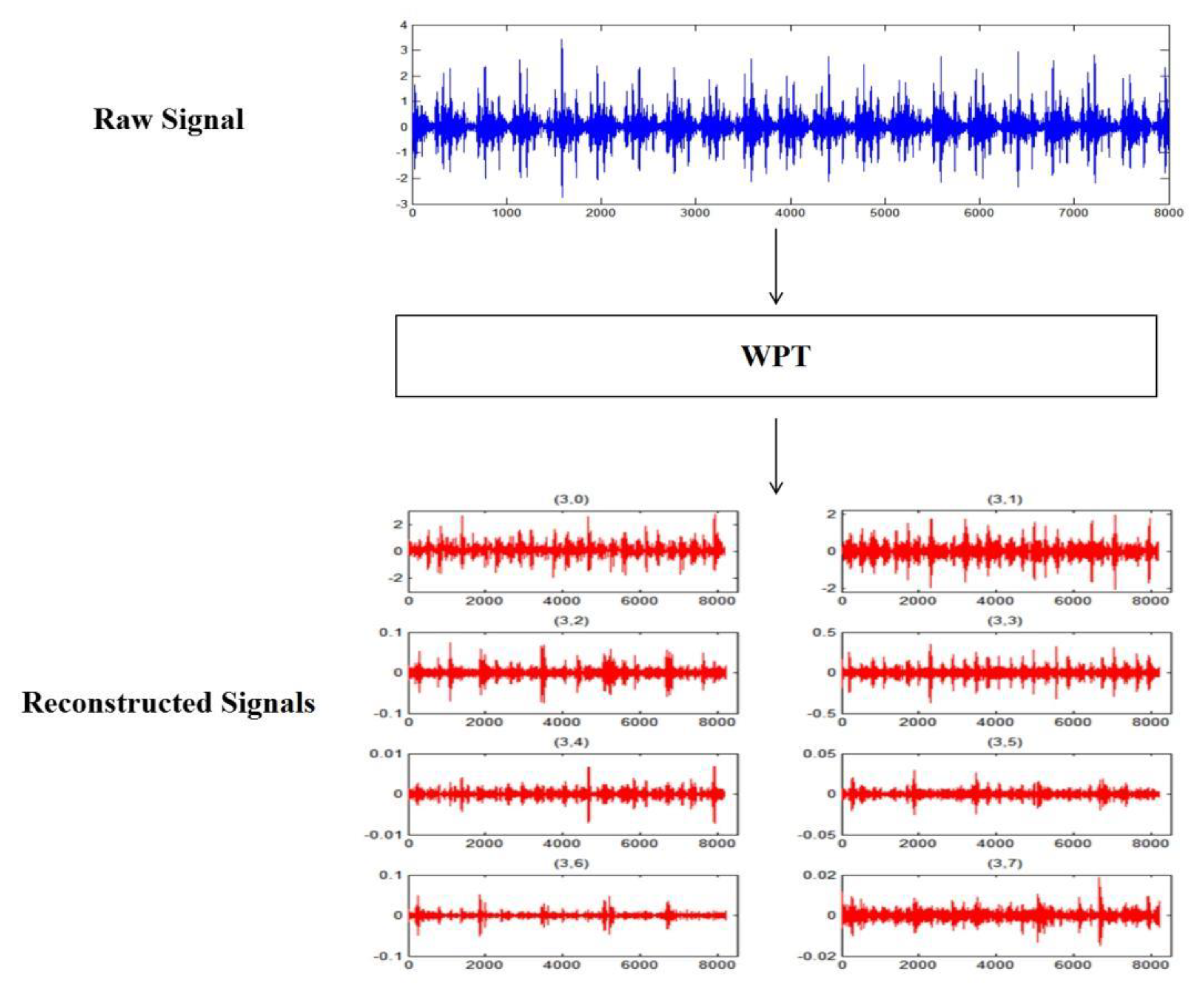
Step 2: Wavelet packet decomposition.

Selecting the appropriate wavelet basis and the number of decomposition layers, each kind of sample data is decomposed into a wavelet packet, and the raw signal is decomposed into a series of reconstructed signals with equal bandwidth.

Step 3: Feature extraction.

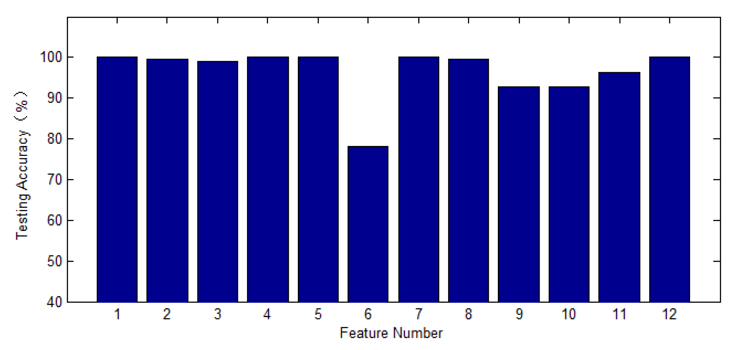
There are m features extracted from the wavelet packet reconstruction signal, and the feature set F = {F₁, F₂,…, F_m} is obtained. The dimension of the feature subset F_j (j = 1, 2, …, m) depends on the number of decomposition layers n by the wavelet packet. In this paper, all the training samples are decomposed by three-layer wavelet packets. Hence, s = 8, and the feature subset can be described as F_j = {F_j¹, F_j², …, F_j⁸}^T.

Step 4: Normalization.

Because neurons are highly sensitive to numbers in the range of [−1, 1], the bearing feature data cannot be directly input into the BPNN, so it is necessary to normalize the feature set. The min–max normalization method is used in this paper.

$$\overline{u}=\frac{u-u_{\min }}{u_{\max }-u_{\min }}$$

(12)

where u and $\overline{u}$ are the original data of the feature set and the normalized data, respectively. u_max is the maximum value in the original feature set, and u_min is the minimum value in the original feature set. Here, u represents the feature value F_j^s and $\overline{u}$ represents the normalized eigenvalue X_j^s.

Step 5: Train BPNNs.

Using the training process detailed in Section 2.2, 5 kinds of training samples are studied, including the bearing state training sample, the fault position training sample, the inner race fault degree training sample, the ball fault degree training sample and the outer race fault degree training sample. A hierarchical decision fusion network of rolling bearings is established capable of fault detection, isolation and fault degree estimation.

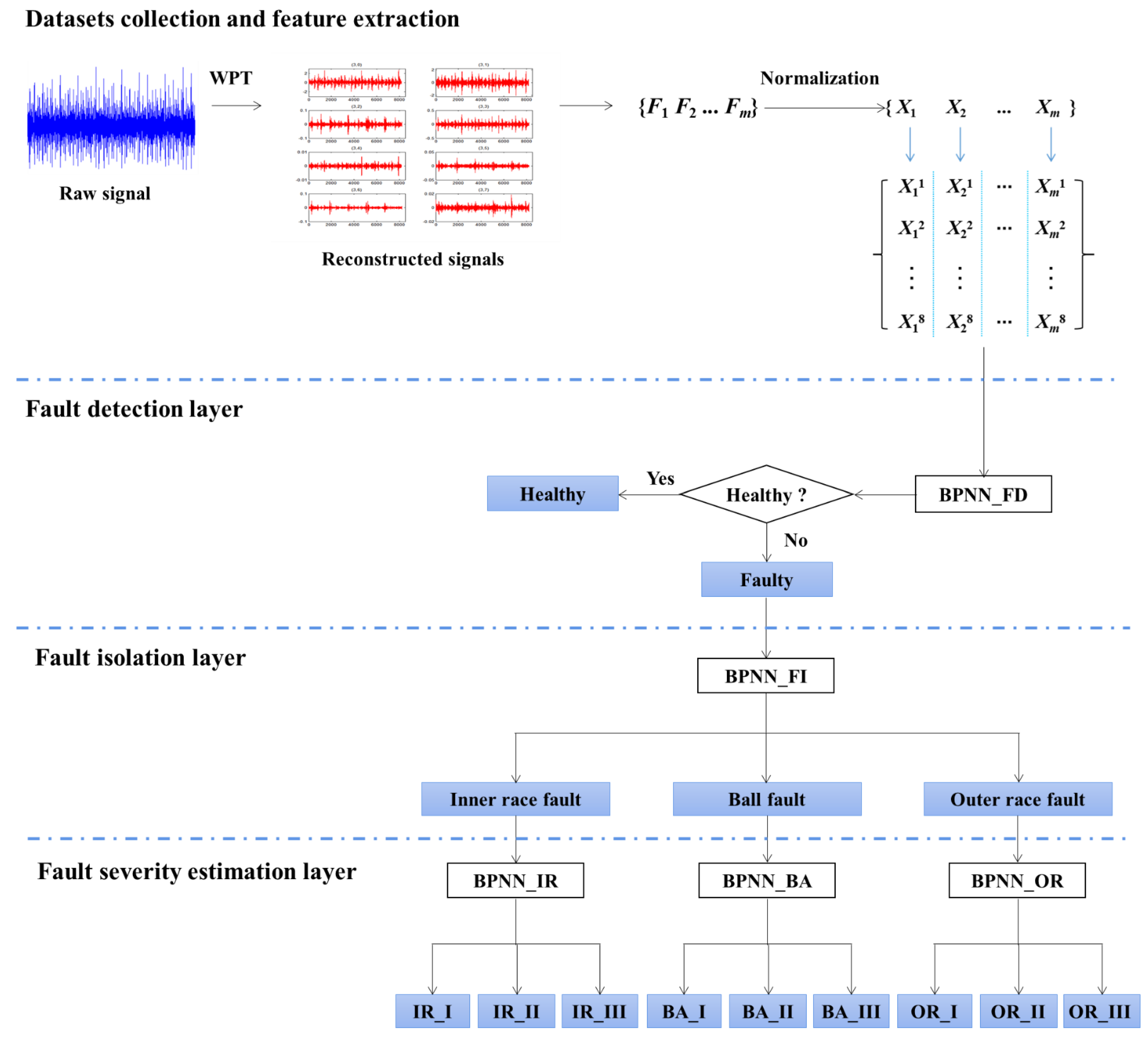
(2) Diagnosis Stage

In the application stage, the flow of the hierarchical decision fusion fault diagnosis method is shown in Figure 5.

Step 1: Database collection and feature extraction

The vibration signals of the rolling bearing are collected in real time. N samples of the same length are randomly sampled from the raw vibration signal. Wavelet packet decomposition and signal reconstruction of data samples are carried out to extract m kinds of features of reconstructed signals and form feature vectors [F₁, F₂, …, F_m]. Finally, the feature vector is normalized.

Step 2: Fault detection

m normalized feature vectors are input into m fault detection neural networks (BPNN_FD), and the current state of the bearing is judged by decision fusion. Step 2 and Step 3 are entered into only when the bearing is in a faulty state. Because most of the bearings are in the normal state during use, such a processing method will reduce the operational burden of the algorithm.

Step 3: Fault isolation

When a bearing is detected as being in a faulty state, m normalized feature vectors are input into m fault isolation neural networks (BPNN_FI). After decision fusion, it can be determined whether the bearing fault has occurred in the inner race, ball or outer race.

Step 4: Fault severity estimation

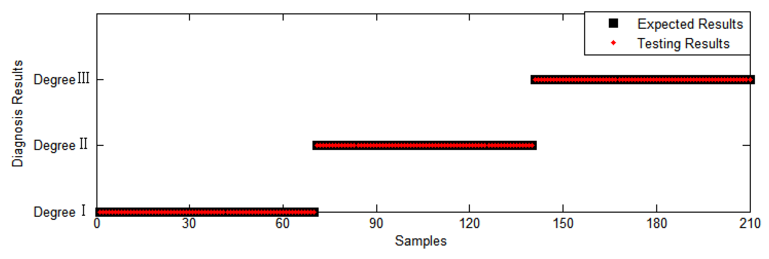
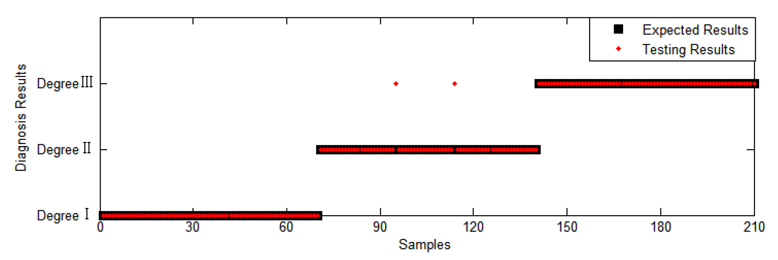
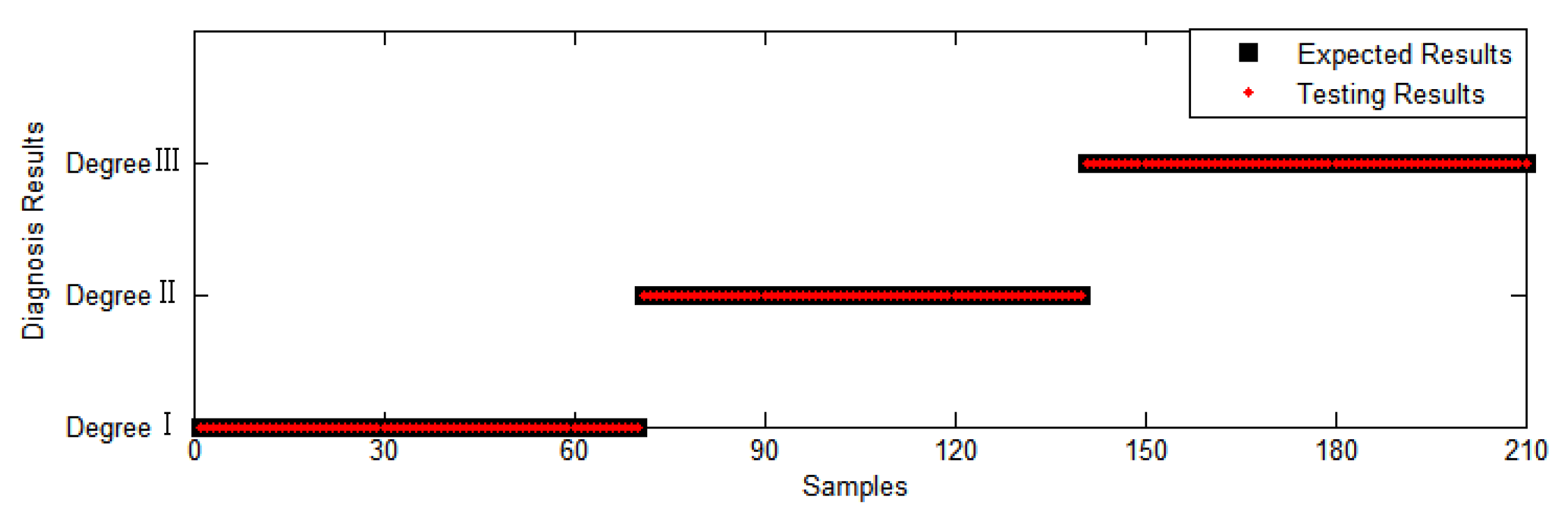
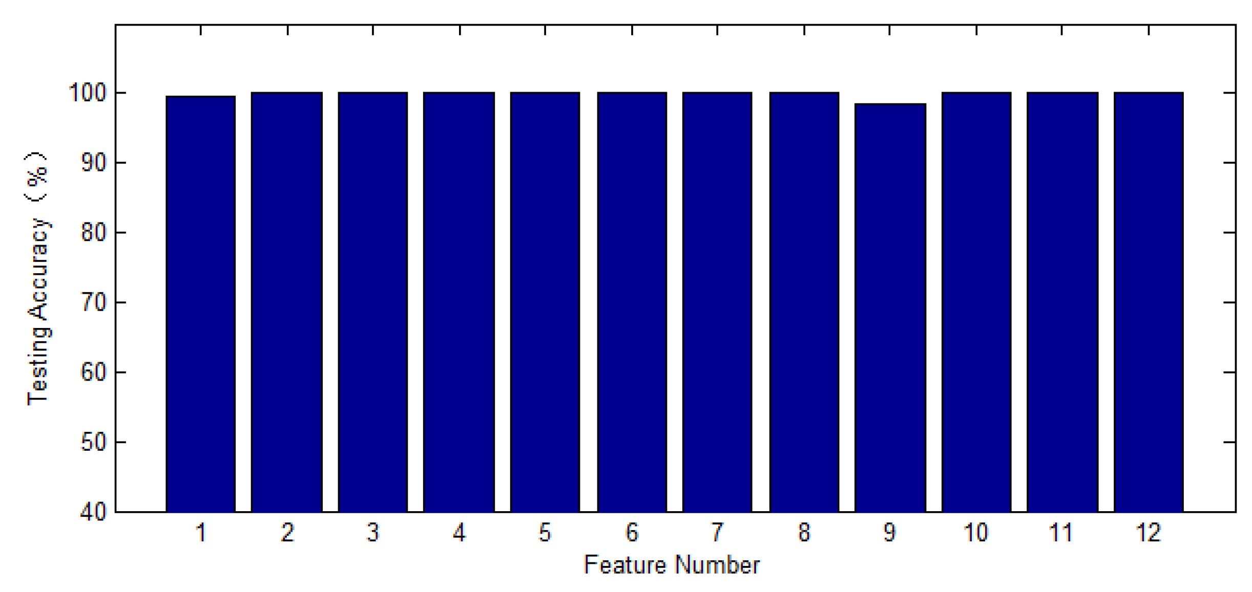
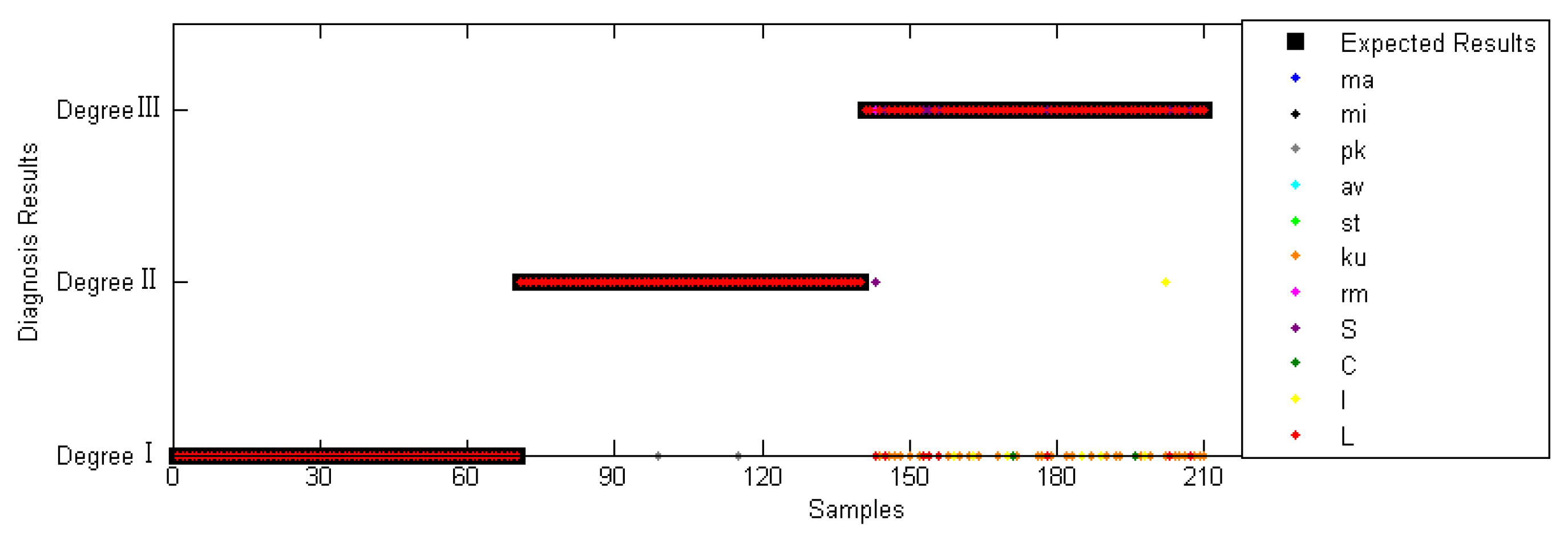
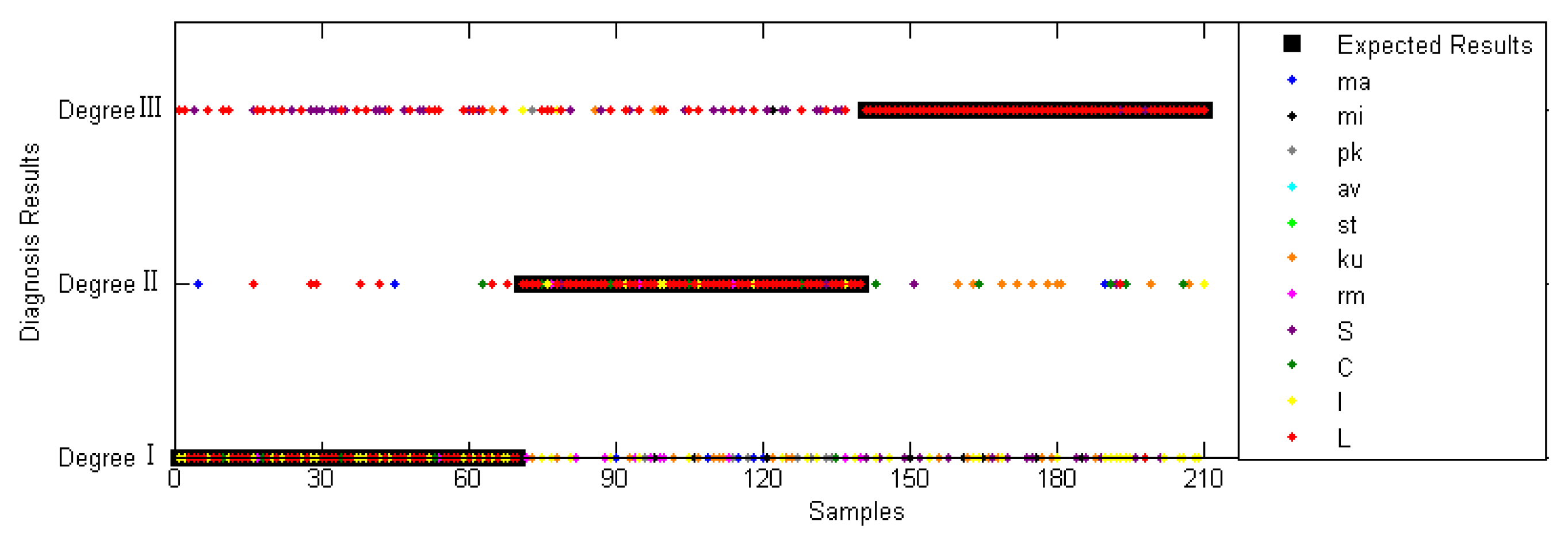
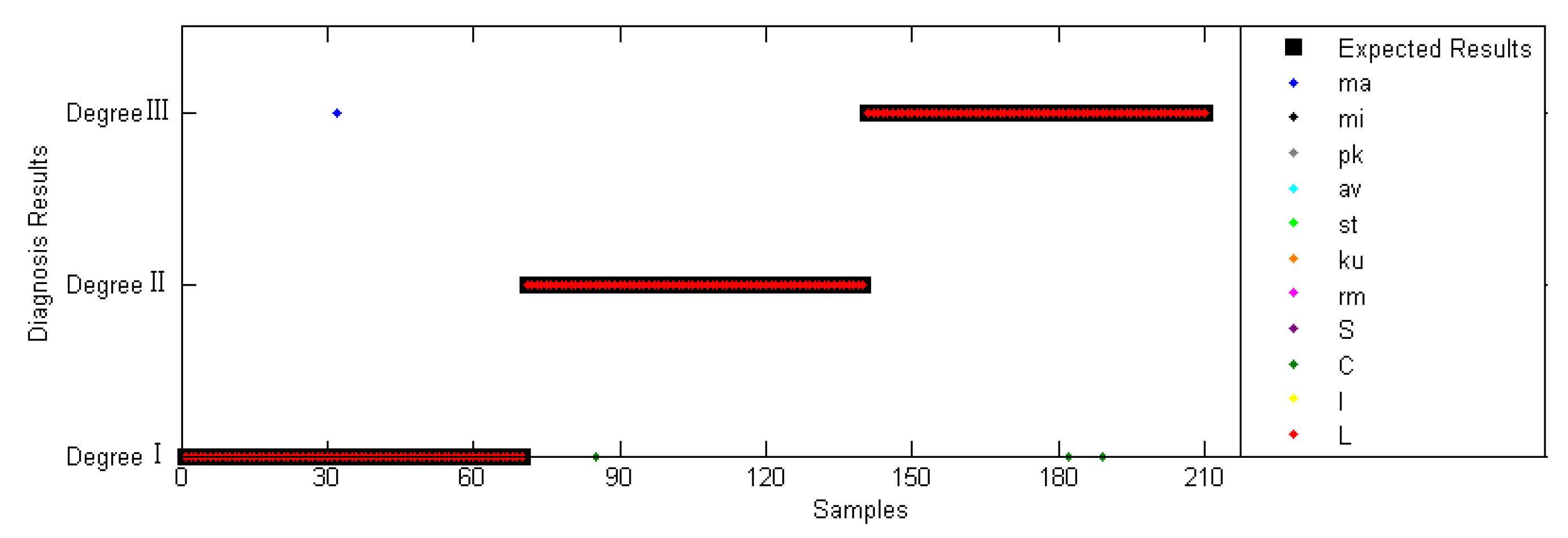
After identifying the location where the bearing fault has occurred, m normalized feature vectors are input to m fault severity estimation neural networks corresponding to the fault location. After decision fusion, the severity of the fault location (degree I, degree II, degree III) is determined. In this paper, there are 11 inner race fault severity estimation neural networks (BPNN_IR), 11 ball fault severity estimation neural networks (BPNN_BA) and 11 outer race fault severity estimation neural networks (BPNN_OR).

3. Case Study

3.1. Experimental Platform

Experimental data was provided by the bearing data center of Western Reserve University [35]. The experiment platform was mainly composed of a motor, torque sensor, power meter and electronic control equipment, as shown in Figure 6. The type of rolling bearing was SKF6205. The single-point faults in the inner raceway, the outer raceway and ball were introduced to the test bearings using electro-discharge machining with fault diameters of 0.007 inches, 0.014 inches and 0.021 inches. Vibration data was collected by using accelerometers, which were installed at the 12 o’clock position at the fan end of the motor housing.

According to the health state, different fault location and different fault degree, the data of 100 segments of length 2048 were randomly selected, generating 10 rolling bearing fault diagnosis sample data sets, as shown in

Table 1. Description of experimental data sets.

Data Set Number	Fault Location	Fault Degree	Fault Diameter (Inches)	Number of Training Samples	Number of Testing Samples
1	Healthy	Healthy	0	30	70
2	Inner race	IR_I	0.007	30	70
3	Inner race	IR_II	0.014	30	70
4	Inner race	IR_III	0.021	30	70
5	Ball	BA_I	0.007	30	70
6	Ball	BA_II	0.014	30	70
7	Ball	BA_III	0.021	30	70
8	Outer race	OR_I	0.007	30	70
9	Outer race	OR_II	0.014	30	70
10	Outer race	OR_III	0.021	30	70

. Each data set contained 30 training samples and 70 test samples. The sampling frequency was 12 kHz, the motor speed was 1797 rpm and the load was 0.

In this paper, the hierarchical decision fusion diagnosis method includes a fault detection layer, a fault isolation layer and a fault severity estimation layer. Each diagnostic layer contains multiple BPNNs. In order to realize the function of these neural networks, it is necessary to train through the corresponding samples, as shown in

Table 2. Sample settings for the fault detection layer.

Name of Network	Classification	Number of Training Samples	Number of Testing Samples	Sources of Data
BPNN_FD	Healthy	30	70	Data set 1
	Faulty	30	70	Data sets 2–10

,

Table 3. Sample settings for the fault isolation layer.

Name of Network	Classification	Number of Training Samples	Number of Testing Samples	Sources of Data
BPNN_FI	Inner race fault	30	70	Data sets 2–4
	Ball fault	30	70	Data sets 5–7
	Outer race fault	30	70	Data sets 8–10

and

Table 4. Sample settings for the fault severity estimation layer.

Name of Network	Classification	Number of Training Samples	Number of Testing Samples	Sources of Data
BPNN_IR	Inner race	30	70	Data set 2
	Inner race	30	70	Data set 5
	Inner race	30	70	Data set 8
BPNN_BA	Ball	30	70	Data set 3
	Ball	30	70	Data set 6
	Ball	30	70	Data set 9
BPNN_OR	Outer race	30	70	Data set 4
	Outer race	30	70	Data set 7
	Outer race	30	70	Data set 10

. Taking the fault detection layer as an example, the output result of the BPNN_FD is healthy or faulty. The total number of training samples was set to 60, where 30 normal samples came from data set 1 in Table 1, and the other 30 fault samples were randomly selected from data sets 2–10.

3.2. Feature Extraction

According to the hierarchical decision fusion diagnosis process of rolling bearings shown in Figure 5, wavelet analysis was used to reconstruct vibration signals. A wavelet basis was chosen as the db4, to decompose the three-layer wavelet packet of vibration signals. Wavelet packet decomposition formed 8 node coefficients, corresponding to 8 frequency band signals, representing all the information of the rolling bearing fault characteristics, as shown in Figure 7. The time-domain features (feature 1–11) of each node reconstructed signal after wavelet packet decomposition were extracted. As shown in

Table 5. Time-domain characteristics of rolling bearings.

Feature Number	Symbol	Time-Domain Feature	Formula
1	Ma	Maximum	Ma = max{x1, x2, …, xn}	(13)
2	Mi	Minimum	Mi = min{x1, x2, …, xn}	(14)
3	Pk	Peak-to-peak value	Pk = Ma − Mi	(15)
4	Av	Average rectified value	$A_v=\frac{1}{n}{\displaystyle \sum _{i=1}^n\left|x_i\right|}$	(16)
5	st	Standard deviation	$st={\left(\frac{1}{n}{\displaystyle \sum _{i=1}^n{(x_i-\overline{x})}^2}\right)}^{\frac{1}{2}}$	(17)
6	ku	Kurtosis	$k_u=\frac{\frac{1}{n}{\displaystyle \sum _{i=1}^n{(x_i-\overline{x})}^4}}{{\left(\frac{1}{n}{\displaystyle \sum _{i=1}^n{(x_i-\overline{x})}^2}\right)}^2}$	(18)
7	rm	Root mean square	$rm=\sqrt{\frac{1}{n}{\displaystyle \sum _{i=1}^n{\left|x_i\right|}^2}}$	(19)
8	S	Waveform factor	S = rm/Av	(20)
9	C	Peak factor	C = Pk/rm	(21)
10	I	Pulse factor	I = Pk/Av	(22)
11	L	Margin factor	$L=P_k/\left(\frac{1}{n}{\displaystyle \sum _{i=1}^n\sqrt{\left|x_i\right|}}\right)$	(23)

, there are 11 features of wavelet packet reconstructed signals.

3.3. Diagnostic Results of Rolling Bearings

3.3.1. Fault Detection Results of Rolling Bearings

Each time-domain feature of each sample of wavelet packet reconstruction signals of rolling bearings is input into the input layer of BPNN, and the fault diagnosis of rolling bearing is carried out by the stratified diagnosis method.

In the rolling bearing fault detection layer, it is determined whether there is a fault in the rolling bearing. According to the sample set of Table 2, the diagnostic accuracy of the fault detection layer based on a single time-domain feature (serial number 1–11) and decision fusion based on a time-domain feature (serial number 12) is tested and compared, as shown in Figure 8.

It can be seen from the diagram that feature 4, feature 5 and feature 7 have a good effect on the diagnosis of wavelet packet reconstruction signal when fault detection is based on a single feature, the diagnosis rate is more than 98% and the diagnosis effect based on other features is relatively poor. When the decision fusion method (number 12) is used to diagnose the fault detection layer, the diagnosis rate increases to 100%, which is a higher diagnostic accuracy than the single-feature-based diagnosis results.

3.3.2. Fault Isolation Results of Rolling Bearings

Assuming that there is a fault in the fault detection layer, it is necessary to isolate the fault of the rolling bearing. According to the testing sample set of Table 3, the location of the fault is diagnosed. The result is shown in Figure 9.

From the diagram, when the bearing is diagnosed based on the average rectified value (feature 4), standard deviation (feature 5) and root mean square (feature 7), the fault diagnosis rate is more than 99.9%. However, for the cases based on kurtosis (feature 6), waveform factor (feature 8), peak factor (feature 9), pulse factor (feature 10) and margin factor (feature 11), the diagnostic accuracy is lower than 70%. When using the decision fusion method (number 12) for fault isolation layer diagnosis, the diagnostic accuracy is 98.57%. Although slightly lower than the highest diagnostic accuracy under a single feature, it is a combination of multiple features, which can avoid the possible error caused by the artificial selection of features. Therefore, a small reduction in diagnostic accuracy caused by decision fusion is acceptable.

3.3.3. Fault Severity Estimation of Rolling Bearings

After the fault location diagnosis of the rolling bearing is obtained in the fault isolation layer, the degree of fault is investigated.

(1) Fault severity estimation results based on single time-domain features

For the same rolling bearing vibration signal sample, the hierarchical diagnosis based on different time-domain features will produce different diagnosis results. This is because the experimental data cannot achieve absolute idealization, it is easy to be interfered with by environmental factors or human factors in the actual experiment, and the selection of data samples also has a certain randomness. According to the test sample set in Table 4, the fault of a bearing may be between two fault degrees, which leads to the hierarchical diagnosis based on different time-domain features and gives different diagnosis results, as shown in Figure 10, Figure 11 and Figure 12. Among them, the black points represent the expected output of the test sample and the other different-colored points represent the diagnosis results of the rolling bearing under different single time-domain features. If the dots of other colors coincide with the black dots, the diagnosis is correct; if not, the diagnosis is misdiagnosed or missed.

(2) Fault severity estimation results based on the decision fusion method

By the decision fusion method, the fault severity estimation results of multiple single time-domain features based on wavelet packet reconstruction signals are fused, and the comprehensive evaluation results of rolling bearing fault severity are obtained, as shown in Figure 13, Figure 14 and Figure 15. The black point represents the expected result based on the decision fusion method, and the red point represents the actual diagnosis result based on the decision fusion method.

(3) The diagnosis result analysis of the fault severity estimation layer

According to the diagnosis results in Figure 10 and Figure 13, the diagnosis results of inner race fault severity under each single feature and fusion decision are obtained, as shown in Figure 16.

It can be seen from the diagram that the diagnostic effect of the wavelet packet reconstruction signal under other single time-domain features is higher than 90%, except for the kurtosis feature (feature 6). In particular, features 1–5, 7 and 8 have an excellent diagnostic effect on the fault severity estimation of the inner race, and the fault diagnosis rate is more than 99%. The result of decision fusion diagnosis under each time-domain feature (number 12) is a fault diagnosis rate of 100% of the wavelet packet reconstructed signal, which is not lower than that of the wavelet packet reconstructed signal under a single feature. This shows that the decision fusion diagnosis method improves the reliability of fault diagnosis of the rolling bearing inner ring to some extent.

According to the diagnosis results in Figure 11 and Figure 14, the diagnosis results of ball fault degree under each single feature and fusion decision are obtained, as shown in Figure 17.

It can be seen from the diagram that there is a big gap in the diagnostic accuracy of ball fault degree based on different single features. Among them, feature 4, feature 5 and feature 7 of the wavelet packet reconstruction signal have a good diagnostic effect on rolling body fault degree, and fault diagnosis accuracy is more than 90%. The diagnostic accuracy based on kurtosis (feature 6) and waveform factor (feature 8) is obviously lower than that based on other single features. The diagnosis results based on each single feature are fused (number 12), and the fault diagnosis accuracy of wavelet packet reconstruction signal is 98.57%.

According to the diagnosis results in Figure 12 and Figure 15, the diagnosis results of outer race fault degree under each single feature and fusion decision are obtained, as shown in Figure 18.

It can be seen from the diagram that when the fault degree of the outer race is identified, the diagnostic accuracy of all single time-domain features for the fault degree of the outer race of the rolling bearing is over 98%. The diagnosis results under each time-domain feature are fused (number 12), and the fault diagnosis rate of wavelet packet reconstruction signal is 100%, which shows that the decision fusion diagnosis method is more comprehensive and reliable than the single-feature diagnosis when diagnosing the fault degree of the outer race of the rolling bearing.

(4) Comparison with other methods

Based on the bearing data of Western Reserve University, the published typical diagnosis results are shown in

Table 6. Comparison with other methods.

Method	Fault Detection Layer	Fault Isolation Layer	Inner Race Degree Layer	Ball Degree Layer	Outer Race Degree Layer	Total
WPE + SVM [36]	-	-	-	-	-	88.9
WPE + CNN [37]	-	-	-	-	-	98.8
CNN + WT [38]	-	-	-	-	-	91.3
BPNN [26]	-	95.23	96.79	99.93	88.74	95.14
SVM [26]	-	96.84	94.14	98.1	96.75	96.48
Method in this paper	100	98.57	100	99.05	100	99.52

. It can be seen that the proposed method not only realizes the accurate detection of bearing faults, but also can accurately locate the fault location and estimate the degree of damage.

3.3.4. The Influence of WPD on Fault Diagnosis

In this paper, the time-domain features in Table 5 of the wavelet packet reconstruction signal of the rolling bearing are extracted, and a stratified diagnosis of the rolling bearing is carried out based on the decision fusion method. In order to prove the positive effect of wavelet packet decomposition and signal reconstruction on fault diagnosis, the time-domain features in Table 5 of raw vibration signals without wavelet packet decomposition are also extracted in this section, and the results of stratified diagnosis are compared in Figure 19. It can be seen from the diagram that after wavelet packet signal reconstruction, the diagnostic accuracy of the rolling bearing in all layers has been improved to different degrees. Therefore, in the fault diagnosis of rolling bearings, wavelet packet signal reconstruction is an effective data preprocessing method and will play a positive role in the diagnosis results.

3.3.5. Fault Diagnosis Results under Variable Load

All the above diagnosis results are based on zero load (HP0) vibration data fault diagnosis. In order to verify the adaptability of the proposed method to load change, the fault data under three constant load conditions, which are 1 horsepower (HP1), 2 horsepower (HP2) and 3 horsepower (HP3), respectively, were input into BPNNs based on zero load data training. Decision fusion diagnosis was used to diagnose rolling bearings.

From

Table 7. Diagnosis result under variable load

Diagnostic Layer		Fault Detection		Fault Isolation		Inner Race Degree		Ball Degree		Outer Race Degree
Signal		Raw Signal	WPT Signal	Raw Signal	WPT Signal	Raw Signal	WPT Signal	Raw Signal	WPT Signal	Raw Signal	WPT Signal
Load	HP0	97.86	100	91.43	98.57	100	100	80.95	99.05	100	100
	HP0→HP1	97.14	98.57	87.9	93.81	96.19	100	72.38	76.19	100	100
	HP0→HP2	98.57	97.14	90.48	89.05	98.1	100	80.48	80.95	100	100
	HP0→HP3	96.43	99.29	86.19	95.24	97.62	100	68.57	70.95	99.52	100

, it can be seen that when the diagnostic condition was extended to other loads, the fault diagnosis in each layer could still reach a higher diagnostic rate, except for the fault degree diagnosis of the ball. Especially for fault detection, inner race fault degree estimation and outer race fault degree estimation, the diagnosis rate did not change too much after changing the working condition to a nonzero load. The proposed method has good adaptability to load change. In addition, the diagnostic rate of wavelet packet reconstruction signal is higher than that of raw vibration signal under the same working condition, which indicates the necessity of wavelet packet reconstruction of the original vibration signal.

4. Conclusions

In this paper, a hierarchical diagnosis method for rolling bearings based on decision fusion is proposed, and bearing data of West Reserve University are used to verify the method. The results show that the proposed method can accurately realize the detection of bearing running state, the isolation of fault position and estimation of the fault severity of the bearing. Because most bearings are in a normal state, so the calculation cost of the proposed method is low. At the same time, the hierarchical diagnosis method only needs to update the related neural networks, which enhances the maintainability of the algorithm. In addition, the proposed method has good adaptability to load change. Compared with the raw vibration signal, the fault detection accuracy is equivalent, but the accuracy of fault isolation and fault severity estimation is obviously improved. The decision fusion is realized by the voting method, which reflects the comprehensive diagnosis results of each characteristic and avoids the missed diagnosis and misdiagnosis caused by the insensitivity of certain characteristics to specific faults. However, whether this method is suitable for bearing multi-fault diagnosis needs further study. In addition, decision fusion considering frequency-domain feature diagnosis results and fusion of different machine learning algorithms need to be further studied.

References

1. Antoni, J.; Borghesani, P. A statistical methodology for the design of condition indicators. Mech. Syst. Signal Process. 2019, 114, 290–327. [Google Scholar] [CrossRef]
2. Wang, Z.; Du, W.; Wang, J.; Zhou, J.; Han, X.; Zhang, Z.; Huang, L. Research and application of improved adaptive MOMEDA fault diagnosis method. Measurement 2019, 140, 63–75. [Google Scholar] [CrossRef]
3. Jiang, H.K.; Xia, Y.; Wang, X.D. Rolling bearing fault detection using an adaptive lifting multiwavelet packet with a 1½ dimension spectrum. Meas. Sci. Technol. 2013, 24, 125002. [Google Scholar] [CrossRef]
4. Randall, R.B.; Antoni, J. Rolling element bearing diagnostics—A tutorial. Mech. Syst. Sig. Process. 2011, 25, 485–520. [Google Scholar] [CrossRef]
5. Gupta, P.; Pradhan, M.K. Fault detection analysis in rolling element bearing: A review. Mater. Today Proc. 2017, 4, 2085–2094. [Google Scholar] [CrossRef]
6. Heng, R.B.W.; Nor, M.J.M. Statistical analysis of sound and vibration signals for monitoring rolling element bearing condition. Appl. Acoust 1998, 53, 211–226. [Google Scholar] [CrossRef]
7. Sawalhi, N.; Randall, R.B. Signal Prewhitening Using Cepstrum Editing (Liftering) to Enhance Fault Detection in Rolling Element Bearings; COMADEM: Stavanger, Norway, 2011. [Google Scholar]
8. Shi, J.; Liang, M.; Necsulescu, D.-S.; Guan, Y. Generalized stepwise demodulation transform and synchro squeezing for time–frequency analysis and bearing fault diagnosis. J. Sound Vib. 2016, 368, 202–222. [Google Scholar] [CrossRef]
9. He, Q.; Ding, X. Sparse representation based on local time-frequency template matching for bearing transient fault feature extraction. J. Sound Vib. 2016, 370, 424–443. [Google Scholar] [CrossRef]
10. Wang, D. Some further thoughts about spectral kurtosis, spectral L2/L1 norm, spectral smoothness index and spectral Gini index for characterizing repetitive transients. Mech. Syst. Signal Process. 2018, 108, 360–368. [Google Scholar] [CrossRef]
11. Han, Z.; Xu, B.; Zhu, X.; Jiao, H. Research on multi-fault diagnosis of rotor based on Approximate entropy and EEMD. China Mech. Eng. 2016, 27, 2186–2189. [Google Scholar]
12. Antoni, J. The infogram: Entropic evidence of the signature of repetitive transients. Mech. Syst. Signal Process. 2016, 74, 73–94. [Google Scholar] [CrossRef]
13. Harish, N.; Sekhar, A.S. Fault detection in rotor bearing systems using time frequency techniques. Mech. Syst. Signal Process. 2016, 72, 105–133. [Google Scholar]
14. Huang, W.; Sun, H.; Luo, J.; Wang, W. Periodic feature-oriented adapted dictionary free OMP for rolling element bearing incipient fault diagnosis. Mech. Syst. Signal Process. 2019, 126, 137–160. [Google Scholar] [CrossRef]
15. Feng, Z.P.; Liang, M.; Zhang, Y.; Hou, S.M. Fault diagnosis for wind turbine planetary gearboxes via demodulation analysis based on ensemble empirical mode decomposition and energy separation. Renew. Energy 2012, 47, 112–126. [Google Scholar] [CrossRef]
16. Zhang, C.; Li, Z.; Hu, C.; Chen, S.; Wang, J.; Zhang, X. An optimized ensemble local mean decomposition method for fault detection of mechanical components. Meas. Sci. Technol. 2017, 28, 035102. [Google Scholar]
17. Antoni, J.; Xin, G.; Hamzaoui, N. Fast computation of the spectral correlation. Mech. Syst. Signal Process. 2017, 92, 248–277. [Google Scholar] [CrossRef]
18. Tham, J.Y.; Shen, L.; Lee, S.L.; Tan, H.H. A general approach for analysis and application of discrete multiwavelet transforms. IEEE Trans. Signal Process. 2000, 48, 457–464. [Google Scholar] [CrossRef]
19. Hosseinabadi, H.Z.; Amirfattahi, R.; Nazari, B.; Mirdamadi, H.R.; Atashipour, S.A. GUW-based structural damage detection using WPT statistical features and multiclass SVM. Appl. Acoust. 2014, 86, 59–70. [Google Scholar] [CrossRef]
20. Wang, Y.; Xiang, J.; Markert, R.; Liang, M. Spectral kurtosis for fault detection, diagnosis and prognostics of rotating machines: A review with applications. Mech. Syst. Signal Process. 2016, 66, 679–698. [Google Scholar] [CrossRef]
21. Zhang, Y.; Randall, R.B. Rolling element bearing fault diagnosis based on the combination of genetic algorithms and fast kurtogram. Mech. Syst. Signal Process. 2009, 23, 1509–1517. [Google Scholar] [CrossRef]
22. Zhou, R.; Bao, W.; Li, N.; Huang, X.; Yu, D. Mechanical equipment fault diagnosis based on redundant second generation wavelet packet transform. Digit. Signal Process. 2010, 20, 276–288. [Google Scholar] [CrossRef]
23. Wang, C. A sample entropy inspired affinity propagation method for bearing fault signal classification. J. Digit. Signal Process. 2020, 102, 1051–2004. [Google Scholar] [CrossRef]
24. Yan, X.; Jia, M. A novel optimized SVM classification algorithm with multi-domain feature and its application to fault diagnosis of rolling bearing. Neurocomputing 2018, 313, 47–64. [Google Scholar] [CrossRef]
25. Lu, C.; Wang, Z.; Zhou, B. Intelligent fault diagnosis of rolling bearing using hierarchical convolutional network based health state classification. Adv. Eng. Inform. 2017, 32, 139–151. [Google Scholar] [CrossRef]
26. Gan, M.; Wang, C. Construction of hierarchical diagnosis network based on deep learning and its application in the fault pattern recognition of rolling element bearings. Mech. Syst. Signal Process. 2016, 72, 92–104. [Google Scholar] [CrossRef]
27. Mao, W.; Liu, Y.; Ding, L.; Li, Y. Imbalanced fault diagnosis of rolling bearing based on generative adversarial network: A comparative study. IEEE Access 2019, 7, 9515–9530. [Google Scholar] [CrossRef]
28. Yang, Y.; Zhang, L.; Zhang, L.; Cai, X.; Zhang, S. The health degree evaluation of rolling element bearings using an improved BP neural network. J. Inf. Comput. Sci. 2012, 9, 4217–4227. [Google Scholar]
29. Zhang, J.; Sun, Y.; Guo, L.; Gao, H.; Song, H. A new bearing fault diagnosis method based on modified convolutional neural networks. Chin. J. Aeronaut. 2019, 33, 439–447. [Google Scholar] [CrossRef]
30. Toma, K.; Dragan, K.; Janez, G. Wavelet packet decomposition to characterize injection molding tool damage. J. Appl. Sci. 2016, 6, 45. [Google Scholar]
31. Asadi, M.; Jamali, M.A.J.; Parsa, S.; Majidnezhad, V. Detecting botnet by using particle swarm optimization algorithm based on voting system. Future Gener. Comput. Syst. 2020, 107, 95–111. [Google Scholar] [CrossRef]
32. Trong, V.H.; Gwang-hyun, Y.; Vu, D.T.; Jin-Young, K. Late fusion of multimodal deep neural networks for weeds classification. Comput. Electron. Agric. 2020, 175, 105506. [Google Scholar] [CrossRef]
33. Tripathi, D.; Edla, D.R.; Cheruku, R. Hybrid credit scoring model using neighborhood rough set and multi-layer ensemble classification. J. Intell. Fuzzy Syst. 2018, 34, 1543–1549. [Google Scholar] [CrossRef]
34. Ghodselahi, A. A hybrid support vector machine ensemble model for credit scoring. Int. J. Comput. Appl. 2011, 17, 1–5. [Google Scholar] [CrossRef]
35. Case Western Reserve University Bearing Data Center Website. Available online: http://csegroups.case.edu/bearingdatacenter/home (accessed on 10 June 2020).
36. Du, W.; Tao, J.; Li, Y.; Liu, C. Wavelet leaders multifractal features based fault diagnosis of rotating mechanism. Mech. Syst. Signal Process. 2014, 43, 57–75. [Google Scholar] [CrossRef]
37. Ding, X.; He, Q. Energy-fluctuated multiscale feature learning with deep convnet for intelligent spindle bearing fault diagnosis. IEEE Trans. Instrum. Meas. 2017, 66, 1926–1935. [Google Scholar] [CrossRef]
38. Verstraete, D.; Ferrada, A.; Droguett, E.L.; Meruane, V.; Modarres, M. Deep learning enabled fault diagnosis using time-frequency image analysis of rolling element bearings. Shock Vib. 2017, 2017, 5067651. [Google Scholar] [CrossRef]
Figure 1. Diagram of wavelet packet decomposition. S: raw signal; A: low-frequency signal; D: high-frequency signal.
Applsci 11 00739 g001
Figure 2. Diagram of Back Propagation Neural Networks (BPNN).
Applsci 11 00739 g002
Figure 3. Decision fusion algorithm based on the voting method.
Applsci 11 00739 g003
Figure 4. Training process of the hierarchical decision fusion fault diagnosis method.
Applsci 11 00739 g004
Figure 5. Hierarchical diagnostic flowchart of rolling bearings.
Applsci 11 00739 g005
Figure 6. Experimental platform of rolling bearing faults.
Applsci 11 00739 g006
Figure 7. Wavelet packet decomposition of raw vibration signal.
Applsci 11 00739 g007
Figure 8. Diagnostic accuracy of fault detection for the rolling bearing. 1: Ma; 2: Mi; 3: Pk; 4: Av; 5: st; 6: ku; 7: rm; 8: S; 9: C; 10: I; 11: L; 12: decision fusion.
Applsci 11 00739 g008
Figure 9. Diagnostic accuracy of fault isolation for the rolling bearing. 1: Ma; 2: Mi; 3: Pk; 4: Av; 5: st; 6: ku; 7: rm; 8: S; 9: C; 10: I; 11: L; 12: decision fusion.
Applsci 11 00739 g009
Figure 10. Diagnosis results of inner race fault severity estimation based on the BPNN_IR network.
Applsci 11 00739 g010
Figure 11. Diagnosis results of ball fault severity estimation based on the BPNN_BA network.
Applsci 11 00739 g011
Figure 12. Diagnosis results of outer race fault severity estimation based on the BPNN_OR network.
Applsci 11 00739 g012
Figure 13. Diagnosis results of inner race fault severity estimation based on the BPNN_IR network and decision fusion.
Applsci 11 00739 g013
Figure 14. Diagnosis results of ball fault severity estimation based on the BPNN_BA network and decision fusion.
Applsci 11 00739 g014
Figure 15. Diagnosis results of outer race fault severity estimation based on the BPNN_OR network and decision fusion.
Applsci 11 00739 g015
Figure 16. Diagnosis result of fault severity of inner race under different features. 1: Ma; 2: Mi; 3: Pk; 4: Av; 5: st; 6: ku; 7: rm; 8: S; 9: C; 10: I; 11: L; 12: decision fusion.
Applsci 11 00739 g016
Figure 17. Diagnosis result of fault severity of ball under different features. 1: Ma; 2: Mi; 3: Pk; 4: Av; 5: st; 6: ku; 7: rm; 8: S; 9: C; 10: I; 11: L; 12: decision fusion.
Applsci 11 00739 g017
Figure 18. Diagnosis result of the fault severity of the outer race under different features. 1: Ma; 2: Mi; 3: Pk; 4: Av; 5: st; 6: ku; 7: rm; 8: S; 9: C; 10: I; 11: L; 12: decision fusion.
Applsci 11 00739 g018
Figure 19. Comparison of fault diagnosis effect of rolling bearings based on decision fusion.
Applsci 11 00739 g019