Sedimentation of Fractal Aggregates in Shear-Thinning Fluids

Abstract

Solid–liquid separation is a key unit operation in the wastewater treatment, generally consisting of coagulation and flocculation steps to promote aggregation and increase the particle size, followed by sedimentation, where the particles settle due to the effect of gravity. The sedimentation efficiency is related to the hydrodynamic behavior of the suspended particles that, in turn, depends on the aggregate morphology. In addition, the non-Newtonian rheology of sludges strongly affects the drag coefficient of the suspended particles, leading to deviations from the known settling behavior in Newtonian fluids. In this work, we use direct numerical simulations to study the hydrodynamic drag of fractal-shaped particles suspended in a shear-thinning fluid modeled by the power-law constitutive equation. The fluid dynamics governing equations are solved for an applied force with different orientations uniformly distributed over the unit sphere. The resulting particle velocities are interpolated to compute the aggregate dynamics and the drag correction coefficient. A remarkable effect of the detailed microstructure of the aggregate on the sedimentation process is observed. The orientational dynamics shows a rich behavior characterized by steady-state, bistable, and periodic regimes. In qualitative agreement with spherical particles, shear-thinning increases the drag correction coefficient. Elongated aggregates sediment more slowly than sphere-like particles, with a lower terminal velocity as the aspect ratio increases.

1. Introduction

Separation of solid particles suspended in liquids is a fundamental operation in the treatment of wastewater. This process generally consists of a sequence of steps, namely, coagulation and flocculation, followed by sedimentation [1]. The first operation aims at destabilizing the suspension through the addition of coagulants that neutralize the negative charges on fine solids. The small destabilized particles are able to come into contact and form larger particles called microflocs. In the flocculation step, the microflocs collide and stick together forming larger and larger particles (macroflocs). Once the suspended aggregates have reached a desired dimension, the suspension undergoes the sedimentation step, i.e., the particles are separated from the liquid through gravity or centrifugal force [2].

The knowledge of the hydrodynamic drag force, which counterbalances the sedimentation force, is crucial to the design and optimization of wastewater treatment plants. Such a force depends on the size and shape of the suspended particles, and on the rheological properties of the liquid. During the flocculation stage, the aggregates assume fractal shapes [3,4,5,6] described by the following equation [7],

$$N_{\mathrm{p}}=k_{\mathrm{f}}{\left(\frac{R_{\mathrm{g}}}{a}\right)}^{D_{\mathrm{f}}}$$

(1)

where $N_{\mathrm{p}}$ is the number of primary particles forming the aggregate, $R_{\mathrm{g}}$ is the radius of gyration, $D_{\mathrm{f}}$ is the fractal dimension, $k_{\mathrm{f}}$ is the fractal pre-factor, and a is the radius of the primary particles. Aggregates with a shape satisfying Equation (1) are referred to as fractal-like or quasi-fractal aggregates, as the scaling law relation is independent of whether the particle has a real scale-invariant (self-similar) morphology [8]. The fractal dimension provides a scaling law between the number of primary particles composing the aggregate and a characteristic cluster size (e.g., the gyration radius). It assumes values between 1 and 3 corresponding to rod-like and spherical-like particles, respectively. The fractal prefactor is a descriptor of the aggregate local structure and is related to the packing factor. Finally, the radius of gyration is a geometric measure of the spatial mass distribution about the aggregate center of mass.

The particle morphology has a relevant influence on the settling velocity, and thus it must be accounted for when dealing with the sedimentation process of flocculated particles [9,10]. Therefore, it is not surprising that the hydrodynamic drag of particles with complex shapes has been thoroughly studied in the literature. Several methodologies have been proposed to compute the hydrodynamic drag of a set of spherical particles in contact, based on expansions of analytical solutions for Stokes flows [11,12,13] or direct numerical simulations [14,15,16]. Due to the linearity of the creeping flow equations, the dynamics of a particle with arbitrary shape can be determined by the mobility tensor that univocally relates translational and angular velocities to the forces and torques acting on the particle [17]. The knowledge of the mobility tensor allows to completely predict the translational and orientational motion of the aggregate. In this regards, it is well known that the settling velocity depends on the aggregate orientation. The average velocity over all possible orientations can be linearly related to the applied force, with a proportionality constant given by the arithmetic mean of the three eigenvalues of the translational mobility tensor divided by the fluid viscosity [13,18,19]. A hydrodynamic radius can be defined as the radius of a sphere that gives the same drag force acting on the aggregate in a uniform flow [13]. It can be readily seen that the hydrodynamic radius is inversely proportional to the aforementioned mean of the eigenvalues of the translational mobility tensor. The knowledge of the hydrodynamic radius for an aggregate with arbitrary shape is, then, sufficient to characterize its average settling velocity. The ratio of the hydrodynamic radius and the gyration radius has been found to be a function of the parameters of the fractal Equation (1) [13,19,20]. Specifically, such a ratio is an increasing function of $D_{\mathrm{f}}$, assuming a value of ~1 for $D_{\mathrm{f}}=2$, up to a limiting value of about 1.29 for $D_{\mathrm{f}}=3$ [13,15,20]. The number of primary particles strongly affects the ratio for low fractal dimensions (rod-like particles), whereas it has a weak influence for more spherical aggregates. Finally, increasing the fractal pre-factor moves the ratio to higher values without altering the dependence on $D_{\mathrm{f}}$ and $N_{\mathrm{p}}$ [13].

All the aforementioned studies consider a Newtonian suspending liquid. In addition, the developed methodologies used to compute the hydrodynamic drag are only applicable to Newtonian fluids. Active sludges, however, show a non-Newtonian rheology [21,22], which has a strong influence on the particle settling dynamics. For a spherical particle in an unbounded shear-thinning inelastic fluid, modeled with the power-law constitutive equation, several works are available showing that the drag force deviates from the Stokes’ law [23,24,25,26]. A drag correction coefficient has been defined as the ratio between the applied force and the Stokes’ drag law, where the viscosity is replaced by the power-law constitutive equation with a characteristic shear rate given by the terminal settling velocity divided by the particle diameter. The coefficient is 1 for a Newtonian fluid and increases as the flow index decreases (i.e., fluid shear-thinning increases). For non-spherical particles, Tripathi et al. [27] carried out finite element simulations to study the flow of a power-law fluid over prolate and oblate spheroidal particles aligned with the flow direction. In this particular orientation, the dependence of the total drag coefficient on the flow index was found to be qualitatively similar to that observed for spherical particles. As the aspect ratio of the prolate spheroid increases, the drag becomes relatively insensitive to the degree of shear-thinning. Oblate spheroids with high aspect ratio experience a lower drag as compared to spheres.

In summary, many works exist dealing with drag calculation of particles with non-spherical shape in Newtonian liquids. Concerning power-law fluids, the only results available are for spheres [25] and spheroids [27], the latter only considering particles oriented with a principal axis along the force direction. To the best of our knowledge, a study on the combined effect of non-Newtonian rheology and complex particle shape on the hydrodynamic drag is missing.

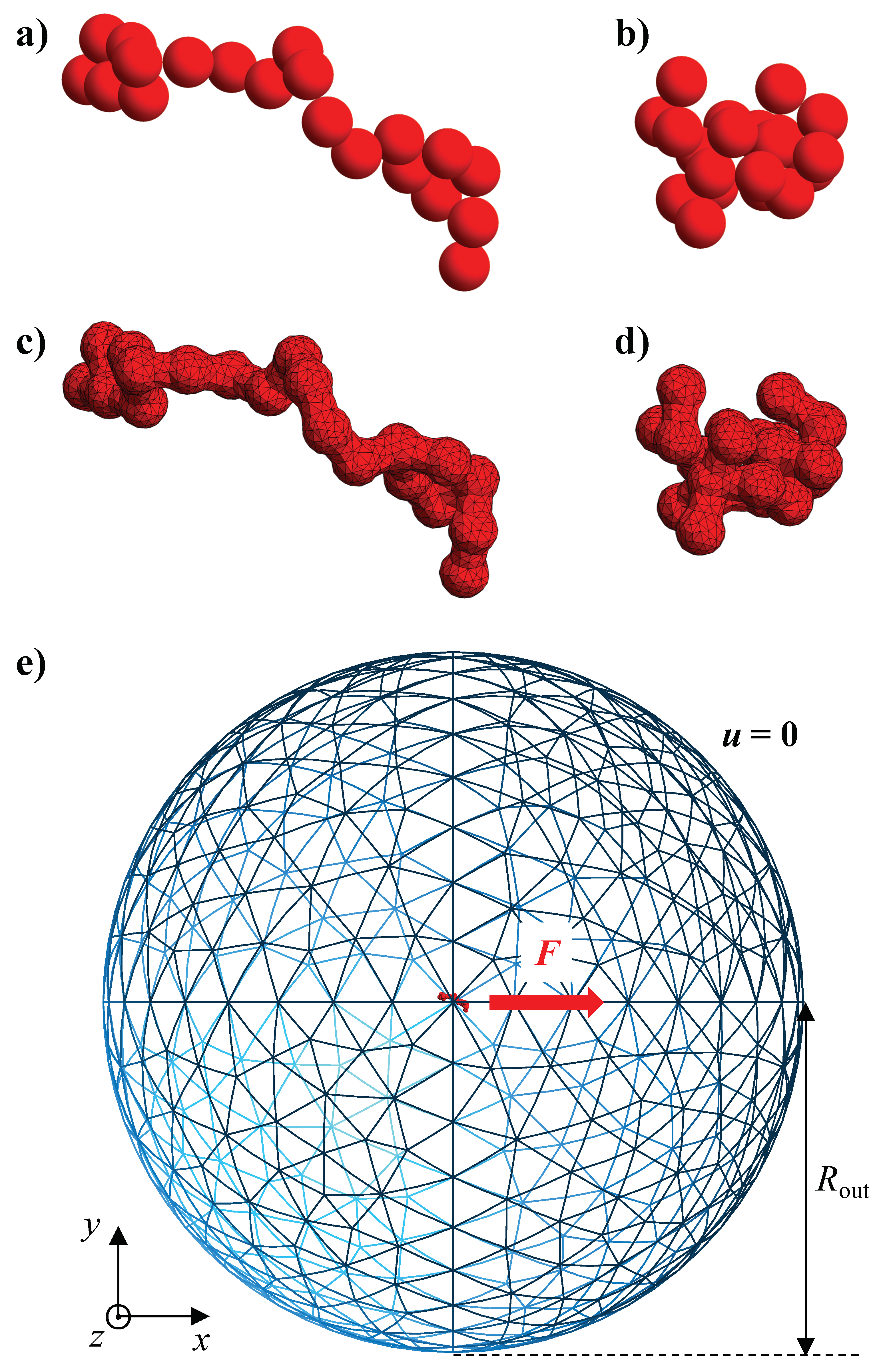
In this work, we investigate the hydrodynamic drag experienced by fractal aggregates suspended in a non-Newtonian fluid by numerical simulations. We assume that the aggregates are sufficiently large to neglect Brownian motion and that their concentration is low enough (less than 5% in volume) to avoid hydrodynamic interactions. This allows us to consider a single-particle problem. The suspending fluid is assumed to be inelastic and shear-thinning, and is modeled by the power-law constitutive equation. A map of particle velocities is precomputed by running finite element simulations for orientations of the applied force uniformly distributed over the unit sphere. Such velocities are then interpolated and used to reconstruct the aggregate dynamics by integrating the evolution equation of the particle position and orientation. The drag correction coefficient at long times is averaged over several initial orientations and particle shapes with the same fractal parameters. The effect of the fractal dimension, the number of primary particles forming the aggregate, and the flow index is investigated.

2. Mathematical Model and Numerical Method

2.1. Governing Equations

A rigid non-Brownian aggregate is suspended in a fluid and subjected to a constant force $\mathit{F}$. The fluid is at rest far from the aggregate. The computational domain, shown in Figure 1e, is a sphere with radius much larger than the maximum size of the particle. The aggregate is placed at the center of the sphere. A Cartesian reference frame is selected with x denoting the direction of the applied force $\mathit{F}$, i.e., $\mathit{F}=(F,0,0)$. The fluid velocity is set to zero on the external spherical surface whereas a rigid-body motion is imposed on the particle boundary. We denote by ${\mathit{x}}_{\mathrm{p}}$ and ${\mathit{\theta }}_{\mathrm{p}}$ the position of the particle center of volume and the rotation angle, and by ${\mathit{U}}_{\mathrm{p}}$ and ${\mathit{\omega }}_{\mathrm{p}}$ the translational and angular particle velocities, respectively. All the symbols used in this work are reported in

Table 1. List of symbols.

a	Radius of primary particles
C	Number of initial aggregate configurations
$\mathit{D}$	Rate-of-deformation tensor
$D_{\mathrm{f}}$	Fractal dimension
$\mathit{f}$	Applied force in the body reference frame
${\mathit{f}}_0$	Initial applied force in the body reference frame
$\mathit{F}$	Applied force in the fixed reference frame
$\mathit{I}$	3x3 unity tensor
$k_{\mathrm{f}}$	Fractal pre-factor
m	Consistency index
n	Flow index
$\mathit{n}$	Unit vector normal to the particle surface
$N_{\mathrm{elem}}$	Number of elements of the tetrahedral mesh
$N_{\mathrm{p}}$	Number of primary particles composing the aggregate
$N_{\mathrm{seed}}$	Number of seeds
p	Fluid pressure
$R_{\mathrm{eff}}$	Radius of a sphere with the same volume of the aggregate
$R_{\mathrm{g}}$	Radius of gyration
$R_{\mathrm{out}}$	Radius of the external sphere
S	Particle surface
t	Time
$\mathit{T}$	Torque on the particle
$\mathit{u}$	Fluid velocity
U	Aggregate velocity along the direction of the applied force
${\mathit{U}}_{\mathrm{p}}$	Particle translational velocity
V	Volume of the aggregate
$\mathit{x}$	Point of particle boundary
${\mathit{x}}_{\mathrm{p}}$	Particle center of volume
${\mathit{x}}_{\mathrm{p},0}$	Initial particle position
X	Drag correction coefficient
$\langle X_{\mathrm{R}}\rangle$	Regime drag correction coefficient
${\langle X_{\mathrm{R}}\rangle }_{\mathrm{m}}$	Ensemble-average drag correction coefficient
$\dot{\gamma }$	Effective deformation rate
$\Delta x$	Size of the elements on the aggregate
$\Delta x_{\mathrm{out}}$	Size of the elements on the external surface
$\eta$	Fluid viscosity
$\theta$	Polar spherical coordinate
${\mathit{\theta }}_{\mathrm{p}}$	Particle rotation angle
${\mathit{\theta }}_{\mathrm{p},0}$	Initial particle rotation angle
$\mathit{\sigma }$	Fluid stress tensor
$\varphi$	Azimuthal spherical coordinate
${\mathit{\omega }}_{\mathrm{p}}$	Particle angular velocity

.

We model the aggregate shape by a set of primary spherical particles with radius a arranged to satisfy the fractal Equation (1). The construction of aggregate shapes satisfying such equation can be done in several ways, for instance by iteratively adding spherical particles (particle–cluster methods) or by directly connecting clusters of particles (cluster–cluster methods) [28,29,30,31,32]. In this work, we adopt the particle–cluster aggregation method proposed in [33,34]. All the available algorithms are based on the generation of pseudorandom numbers. Therefore, infinite shapes for the same fractal parameters can be obtained by changing the seed of the random number generator. We report in Figure 1 two examples of structures generated with $N_{\mathrm{p}}=20$, $k_{\mathrm{f}}=1.3$, and $D_{\mathrm{f}}=1.5$ (Figure 1a) or $D_{\mathrm{f}}=2.5$ (Figure 1b).

Assuming negligible fluid and particle inertia, the fluid dynamics of the investigated system is governed by the following mass and momentum balance equations,

$$\begin{array}{c}\nabla ·\mathit{u}=0\end{array}$$

(2)

$$\begin{array}{c}\nabla ·\mathit{\sigma }=\mathbf{0}\end{array}$$

(3)

$$\begin{array}{c}\mathit{\sigma }=-p\mathit{I}+2\eta \left(\dot{\gamma }\right)\mathit{D}\end{array}$$

(4)

where $\mathit{u}$, $\mathit{\sigma }$, p, $\mathit{I}$, $\eta$, and $\mathit{D}$ are the velocity vector, the stress tensor, the pressure, the $3\times 3$ unity tensor, the fluid viscosity, and the rate-of-deformation tensor $\mathit{D}=(\nabla \mathit{u}+{(\nabla \mathit{u})}^{\mathrm{T}})/2$, respectively. We model the suspending fluid by the power-law constitutive equation:

$$\eta \left(\dot{\gamma }\right)=m{\dot{\gamma }}^{n-1}$$

(5)

where m is the consistency index, n is the flow index, and $\dot{\gamma }=\sqrt{2\mathit{D}:\mathit{D}}$ is the effective deformation rate. This model predicts shear-thinning for $n<1$. For $n=1$, a Newtonian fluid with (constant) viscosity m is recovered.

The fluid is at rest far from the aggregate and rigid-body motion is applied at the particle boundary, resulting in the following boundary conditions at the external spherical surface,

$$\mathit{u}=\mathbf{0}$$

(6)

and at the surface of the aggregate,

$$\mathit{u}={\mathit{U}}_{\mathrm{p}}+{\mathit{\omega }}_{\mathrm{p}}\times (\mathit{x}-{\mathit{x}}_{\mathrm{p}})$$

(7)

with $\mathit{x}$ a point of the particle boundary.

Finally, we need to specify the hydrodynamic total force and torque acting on the aggregate. Under the assumption of inertialess particle, the following equations hold,

$$\begin{array}{c}\mathit{F}={\int }_S\mathit{\sigma }·\mathit{n}dS\end{array}$$

(8)

$$\begin{array}{c}\mathit{T}={\int }_S(\mathit{x}-{\mathit{x}}_{\mathrm{p}})\times (\mathit{\sigma }·\mathit{n})dS=\mathbf{0}\end{array}$$

(9)

where $\mathit{T}$ is the total torque on the particle surface S and $\mathit{n}$ is the unit vector normal to the particle surface pointing from the fluid to the boundary. Notice that the aggregate is torque-free, whereas the only external force is the applied force $\mathit{F}$.

The solution of the governing equations gives the fluid velocity and pressure fields, along with the particle translational and angular velocities. The translational and orientational dynamics can be computed by integrating the following equations,

$$\begin{array}{c}\frac{d{\mathit{x}}_{\mathrm{p}}}{dt}={\mathit{U}}_{\mathrm{p}}\end{array}$$

(10)

$$\begin{array}{c}\frac{d{\mathit{\theta }}_{\mathrm{p}}}{dt}={\mathit{\omega }}_{\mathrm{p}}\end{array}$$

(11)

with initial conditions ${\mathit{x}}_{\mathrm{p}}{|}_{t=0}={\mathit{x}}_{\mathrm{p},0}$ and ${\mathit{\theta }}_{\mathrm{p}}{|}_{t=0}={\mathit{\theta }}_{\mathrm{p},0}$. Notice that, for the problem under investigation (settling dynamics of a particle in an unbounded fluid), the evolution of the aggregate center of volume does not affect the orientational dynamics. Therefore, Equation (10) can be removed from the set of equations to be solved.

The governing equations can be made dimensionless by choosing appropriate characteristic quantities for length, time, and stress. As characteristic length, we choose the effective radius of the aggregate, defined as the radius of a sphere with the same volume V of the aggregate, $R_{\mathrm{eff}}={\left(\frac{3V}{4\pi }\right)}^{1/3}$. The characteristic time is chosen as the inverse of a characteristic shear rate ${(U/R_{\mathrm{eff}})}^{-1}$, where U is the velocity along the direction of the applied force. The characteristic stress is $m{(U/R_{\mathrm{eff}})}^n$. By using such characteristic quantities, we can recast the governing equations and boundary conditions in their dimensionless form. In these equations, only the flow index n appears as dimensionless parameter. Therefore, the investigated system is fully determined by specifying n and the geometry of the aggregate defined by the parameters in Equation (1). In this regard, the radius of the primary particles a is related to $R_{\mathrm{eff}}$ through $N_{\mathrm{p}}$. Moreover, the radius of gyration $R_{\mathrm{g}}$ is determined once the other three parameters in Equation (1) are chosen. Therefore, the geometrical parameters that need to be specified are the number of particles $N_{\mathrm{p}}$, the fractal dimension $D_{\mathrm{f}}$, and the fractal pre-factor $k_{\mathrm{f}}$.

To quantify the hydrodynamic resistance of the particle to the applied force, we introduce the drag correction coefficient [25]:

$$X=\frac{F}{6\pi m{\left(\frac{U}{2R_{\mathrm{eff}}}\right)}^{n-1}U{R}_{\mathrm{eff}}}$$

(12)

defined as the applied force divided by the modified Stokes drag coefficient where the Newtonian viscosity is replaced by the power-law model. Of course, $X=1$ for a sphere in a Newtonian fluid. The value of X depends on the orientation of the aggregate and, as such, changes in time since the particle varies its orientation while sedimenting. As it will be discussed below, the aggregate orientation can achieve various regimes, leading to different regime drag correction coefficients $X_{\mathrm{R}}$. As $X_{\mathrm{R}}$ is affected by the initial particle orientation, we average over C initial configurations:

$$\langle X_{\mathrm{R}}\rangle =\frac{1}{C}\sum _C{X}_{\mathrm{R}}$$

(13)

Finally, to make the results independent of the seed used in the algorithm to generate the aggregate, for each set of fractal parameters in Equation (1), the simulation is repeated with different seeds. The ensemble-average drag correction coefficient is computed as

$${\langle X_{\mathrm{R}}\rangle }_{\mathrm{m}}=\frac{1}{N_{\mathrm{seed}}}\sum _{N_{\mathrm{seed}}}\langle X_{\mathrm{R}}\rangle$$

(14)

with $N_{\mathrm{seed}}$ the number of seeds.

In this work, the fractal pre-factor is fixed to $k_{\mathrm{f}}=1.3$, which is a value commonly used in the literature to describe realistic aggregate shapes [8]. The sedimentation dynamics is studied by varying the flow index, the fractal dimension, and the number of primary spheres forming the particle.

2.2. Numerical Method

The calculation of the regime drag correction coefficient requires the knowledge of the orbit followed by the aggregate while pulled by the force. This would need, at each time step, the calculation of the particle angular velocity from the solution of the set of equations presented in the previous section (as discussed above, the translational dynamics is irrelevant). Instead of directly solving the governing equations to compute the orbit, we can greatly speed-up the calculations by precomputing a database of particle translational and angular velocities for different orientations of the aggregate [35,36]. The velocities needed at the right-hand side of Equations (10) and (11) are, then, obtained by interpolating the data of the database. In this way, the computational effort is only due to the construction of the database that can be used to compute the orbit for any initial orientation. Of course, the database must be re-computed for every particle morphology.

Due to the irregular particle shape, two orthogonal vectors fixed with the particle are needed to track the evolution of its orientation. However, it should be noted that any configuration obtained by rotating the aggregate around the applied force is equivalent in terms of particle dynamics and drag coefficient. Consequently, one orientation vector is sufficient to fully describe all the possible configurations of the aggregate with respect to the applied force. This can be readily seen if we consider the particle fixed in the laboratory frame and the applied force is rotated. All the possible configurations are, indeed, obtained by rotating the applied force around the unit sphere (so just considering one orientation vector). This is, in fact, the procedure we adopted to build the database, i.e., we fix the aggregate orientation as generated by the particle–cluster algorithm and solve the fluid dynamics problem for several orientations of the applied force uniformly distributed over the unit sphere. More specifically, we divide the unit sphere in a triangular mesh with icosahedral symmetry. The orientations of the force are taken as the directions connecting the center of the unit sphere and the vertices of the icosahedral mesh. We select an icosahedral subdivision with 162 vertices, verifying that this subdivision is sufficient to assure a good accuracy of the interpolation. Indeed, by computing the interpolating functions on an icosahedral grid with 42 vertices, the maximum relative error is ~3%.

Once the database of particle velocities (and the corresponding drag correction coefficients) has been computed, the rotational dynamics of the aggregate can be calculated by integrating Equation (11). It is, however, more convenient to compute the particle dynamics in the body reference frame, i.e., by fixing the orientation of the particle and rotating the applied force. The adopted procedure is summarized in Algorithm 1. We have denoted with $\mathit{f}$ the (time-dependent) applied force vector acting on the aggregate, and with ${\mathit{f}}_0$ its initial value. In step 3, the search procedure described in [37] is used. A linear interpolation over the spherical triangle mesh is done in step 4 [37,38]. The update of the force $\mathit{f}$ is carried out through quaternions [39]. Specifically, in step 5, a third-order Adams–Bashforth scheme is used to integrate in time the quaternions through the angular velocity computed at the previous step. A rotation matrix in terms of quaternions is constructed and used to update $\mathit{f}$. The procedure just described gives the time-evolution of the applied force $\mathit{f}$ and of the drag correction coefficient $X\left(t\right)$ that can be used to calculate the regime drag correction coefficient $X_{\mathrm{R}}$. Finally, the aggregate orbit can be reconstructed by transforming the force from the body to the lab reference frame, i.e., by rotating the aggregate according to the rotation matrix that, at every instant, transform $\mathit{f}$ in $\mathit{F}=(F,0,0)$ (that is the applied force in the lab frame). The procedure summarized in Algorithm 1 has been adopted to simulate the rheology of a dilute suspension of fractal aggregates in shear-thinning fluids and validated by reproducing the dynamics of spheroids in shear flow [36].

Algorithm 1. Procedure used to update the applied force in the body reference frame.

1:  ${\mathit{f}}_0\leftarrow$ initial orientation of the force

2: for $t\leftarrow 1,num\_time\_steps$ do

3:   Identify the spherical triangle containing $\mathit{f}$

4:   Compute ${\omega }_{\mathrm{p}}$ and X through interpolation over the spherical triangle in $\mathit{f}$

5:   Update $\mathit{f}$ using quaternions

6: end for

The solution of the governing equations to build the database is done by the finite element method. The particle translational and angular velocities are treated as additional unknowns, and are included in the weak form of momentum equation. Lagrange multipliers in each node of the particle surface are employed to enforce the conditions in Equations (8) and (9) [40,41]. The fluid domain is discretized by tetrahedral elements. Mesh generation issues arise due to the contact points between the spheres generated by the particle–cluster algorithm. To overcome this problem, we perform a Boolean union operation of the spheres with a set of cylinders connecting the centers of the spheres in contact. The radius of the cylinders is $0.732a$. We checked that lower values of the cylinder radius do not significantly alter the results. The Boolean union, smoothing, and meshing of the aggregate surface is done by the library PyMesh [42]. Examples of the surface meshes for the aggregates in Figure 1a,b are shown in Figure 1c,d. The tetrahedral volume mesh is generated by Gmsh [43].

The mesh and geometrical parameters used in the simulations are reported in

Table 2. Mesh and geometrical parameters.

${\mathit{N}}_{\mathbf{p}}$	$\mathbf{\Delta }\mathit{x}$	${\mathit{R}}_{\mathbf{out}}$	$\mathbf{\Delta }{\mathit{x}}_{\mathbf{out}}$	${\mathit{N}}_{\mathbf{elem}}$
20	0.25	200	35	∼25,000
50	0.25	400	60	∼60,000
100	0.35	800	120	∼60,000

for the three values of $N_{\mathrm{p}}$ considered in this work. The symbols $\Delta x$, $\Delta x_{\mathrm{out}}$, and $R_{\mathrm{out}}$ denote the size of the elements on the aggregate surface and on the external domain (made dimensionless by the primary particle radius a), and the radius of the external sphere (see Figure 1e). The number of tetrahedral elements $N_{\mathrm{elem}}$ is reported in the last column of Table 2. Notice that, to neglect the effect of the boundary condition far from the particle, very large external domains are needed. Furthermore, as expected, bigger aggregates (i.e., higher values of $N_{\mathrm{p}}$) require larger external domains. We verified mesh and domain size convergence by reducing both $\Delta x$ and $\Delta x_{\mathrm{out}}$, and by further increasing $R_{\mathrm{out}}$. The (dimensionless) time-step size depends on the flow index n, ranging from about $0.01$ for $n=1$ to $0.005$ for $n=0.6$.

The accuracy of the finite element solution is checked by comparing the results for a spherical particle in a power-law fluid with those reported in Dazhi and Tanner [25]. In Figure 2, the drag correction coefficient is reported as a function of the flow index n. The black circles are the simulation results by Dazhi and Tanner [25] and the triangles are obtained by our simulations for different mesh resolutions and size of the external domain (the radius of the spherical particle is 1, meshes M1 and M2 have approximately 50,000 and 70,000 elements). First of all, the superposition of the triangles denotes that the results are independent of the mesh and domain size used. A fair agreement between triangles and circles is observed for values of the flow index between 0.8 and 1. For lower n-values, deviations between the two sets of data are observed. We believe this is due to the coarser mesh used in Dazhi and Tanner that is particularly problematic for low values of the flow index due to large gradients of the velocity field around the particle. We have further examined this point by solving the same problem in a 2D axisymmetric geometry allowing for a much more refined mesh. The results show that the data for an extremely fine mesh overlap the triangles (deviations are lower than $1\%$). Furthermore, by progressively coarsening the mesh, the value of X moves towards the black circles. It should be noted, however, that the maximum deviation between the triangles and the circles (at $n=0.4$) is ~$4\%$, which is a relatively low value.

3. Results

We investigate the aggregate dynamics and the resulting drag correction coefficient by varying the fractal dimension, the flow index, and the number of primary particles forming the aggregate. The values selected for the three parameters are $D_{\mathrm{f}}=[1.5,2.0,2.5]$, $n=[1.0,0.8,0.6]$, and $N_{\mathrm{p}}=[20,50,100]$. As discussed in Section 2.2, for each set of these parameters, we first run single-step simulations for different orientations of the applied force uniformly distributed over the unit sphere. 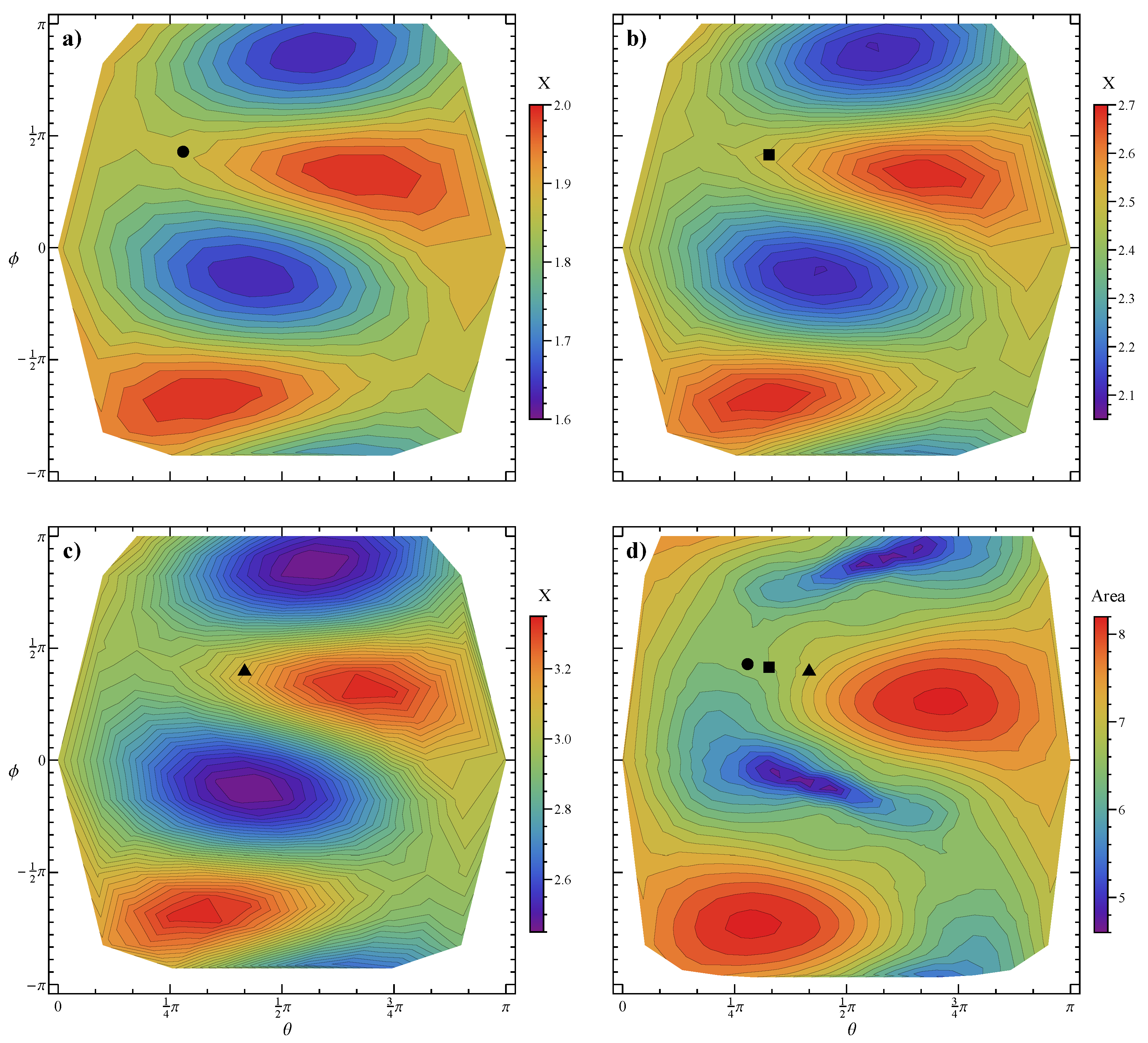Figure 3a–c reports the drag correction coefficient X as a function of the polar and azimuthal spherical coordinates $(0\le \theta \le \pi ,-\pi \le \varphi \le \pi )$, identifying the orientation of the applied force for $n=1$ (i.e., the Newtonian case), $n=0.8$, and $n=0.6$, respectively. The aggregate is the one shown in Figure 1a, i.e., with $N_{\mathrm{p}}=20$ and $D_{\mathrm{f}}=1.5$. It can be readily observed that (i) the drag correction coefficient depends on the orientation of the force; (ii) the distributions are symmetric since X is the same for a specific force orientation $(\theta ,\varphi )$ and its opposite $(\pi -\theta ,\varphi \pm \pi )$; (iii) in agreement with the spherical particle case [25], the drag correction coefficient increases as the flow index decreases (see the bar legends on the right of the panels); and (iv) the distributions are not affected by the flow index (for instance, the maxima and minima are observed for the same orientations of the force). Previous results have evidenced a trend between the drag force experienced by a fractal aggregate and its area projected along the direction of the applied force [14], although this geometrical quantity is not sufficient to accurately predict the drag. The dimensionless area of the aggregate projected along the force direction is reported in Figure 3d. Specifically, we take the directions identified by the 162 vertices of the unity sphere and, for each of them, we compute the area of the aggregate projected on a plane orthogonal to that direction (identified by the spherical coordinates $\theta$ and $\varphi$). The comparison with panels (a)–(c) shows some similarities between the distributions, e.g., the position of the maxima and minima is approximately the same, although a strict correlation is not observed.

The same quantities are reported in Figure 4 for the more sphere-like aggregate in Figure 1b ($N_{\mathrm{p}}=20$, $D_{\mathrm{f}}=2.5$). As for the previous case, similar distributions are observed as the flow index is varied, with higher values of X for more shear-thinning fluids. The projected area also shows a trend similar to the drag correction coefficient. Due to the higher value of the fractal dimension leading to an aggregate with a more spherical shape, the range of variation of both the projected area and the drag correction coefficient is narrower than in the case at $D_{\mathrm{f}}=1.5$, i.e., the influence of the force orientation is weaker.

The data presented so far refer to the instantaneous drag correction factor, i.e., the one obtained by solving the fluid dynamics equations for a fixed orientation of the force (or, equivalently, of the aggregate for a fixed force). The applied force, however, generates a rotation of the aggregate (and, of course, a translation) leading to a change of the orientation and, in turn, of the drag correction coefficient. The knowledge of the orientational dynamics of the aggregate is then crucial to determine the time evolution of the drag correction coefficient and the regime attained by the particle. By using the procedure described in the previous section, we compute the orientational dynamics of the applied force for different initial orientations. Figure 5 shows the orbits for the aggregates reported in Figure 1a (top row) and Figure 1b (bottom row), and for the Newtonian (left column) and power-law fluid with $n=0.6$ (right column). Twelve initial orientations uniformly distributed over the unit sphere are considered (blue circles). For these sets of parameters, the orbits converge towards a unique equilibrium point (green circle) regardless of the initial orientation. In the fixed reference frame, this means that the aggregate achieves a stable orientation. Specifically, our simulations show that, once the regime is achieved, the particle still rotates around the applied force, although with a very small rotation rate (the resulting linear velocity, obtained as the angular velocity around the applied force times the effective radius, is 2–3 orders of magnitude smaller than the sedimentation velocity). It is important to point out, however, that this rotation does not influence the drag as any configuration around the force is equivalent (i.e., the force direction is a symmetry axis). The orientations of the force corresponding to the equilibrium points (green circles in Figure 5) are shown as symbols in the previous Figure 3 and Figure 4. It can be readily observed that shear-thinning slightly affects the equilibrium orientation only for rod-like particles, whereas it has no influence for higher values of the fractal dimension (the symbols in Figure 4 overlap). Moreover, in both cases, the equilibrium orientation does not correspond to any special value of the projected area (for instance the minimum). Therefore, this quantity is not representative of the final orientation achieved by the aggregate and, as such, it is not helpful to estimate the drag correction factor at long times. On the contrary, the detailed microstructure of the aggregate needs to be considered to correctly predict the sedimentation dynamics.

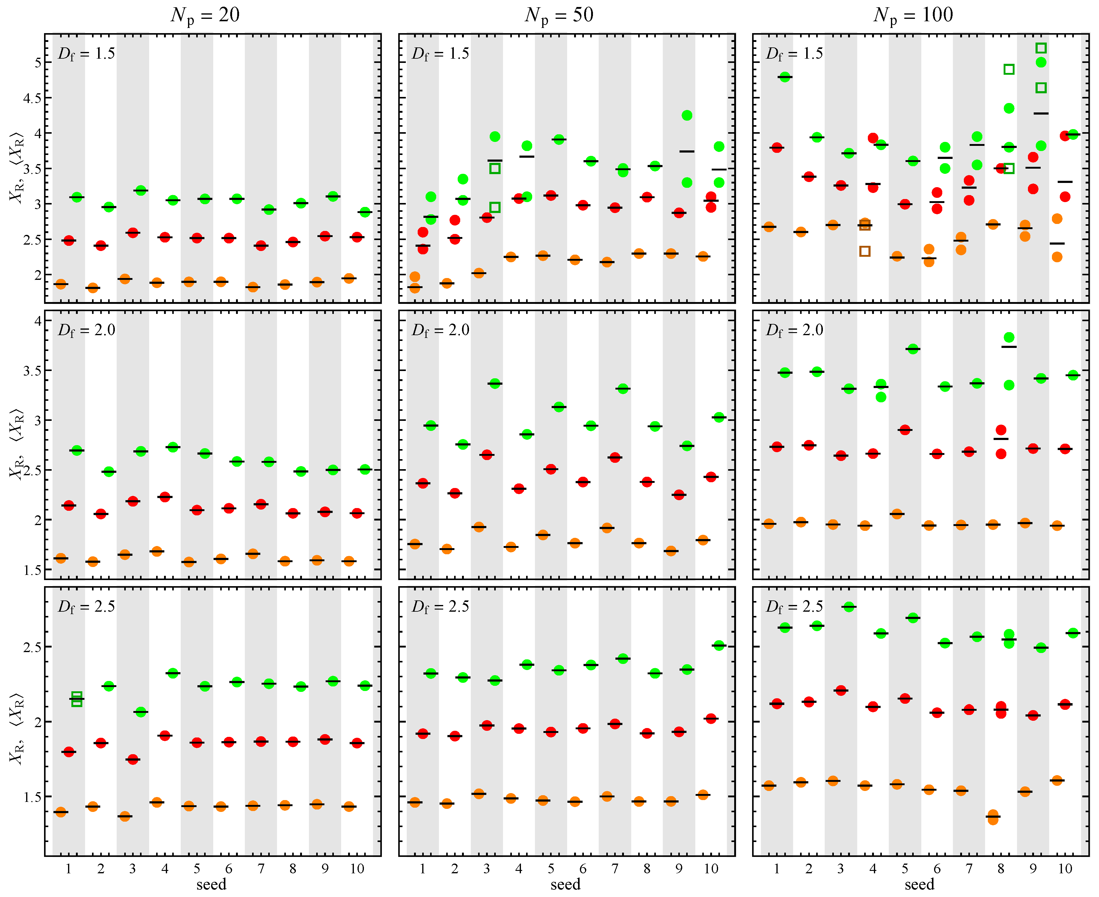
To further investigate on the effect of aggregate morphology, we have repeated the calculations by varying the seed of the random number generator. We recall that, although the fractal parameters in Equation (1) are fixed, the morphologies obtained by varying the seed are different. In the leftmost panels of Figure 6, the regime drag correction coefficient is shown as a function of the seed for $N_{\mathrm{p}}=20$ and for different values of the fractal dimension and the flow index. If the force reaches an equilibrium point, regardless of the initial orientation like the orbits shown in Figure 5, $X_{\mathrm{R}}$ is taken as the steady-state value. These points are represented as solid circles in Figure 6. The data show that, for $N_{\mathrm{p}}=20$, the specific morphology (seed) has a relatively weak effect on $X_{\mathrm{R}}$, with a maximum relative deviations of 7% from the average value. Furthermore, in all the investigated cases, a single equilibrium orientation is achieved, except in one case ($D_{\mathrm{f}}=2.5$, $\mathrm{seed}=1$, and $n=0.6$) that will be discussed later.

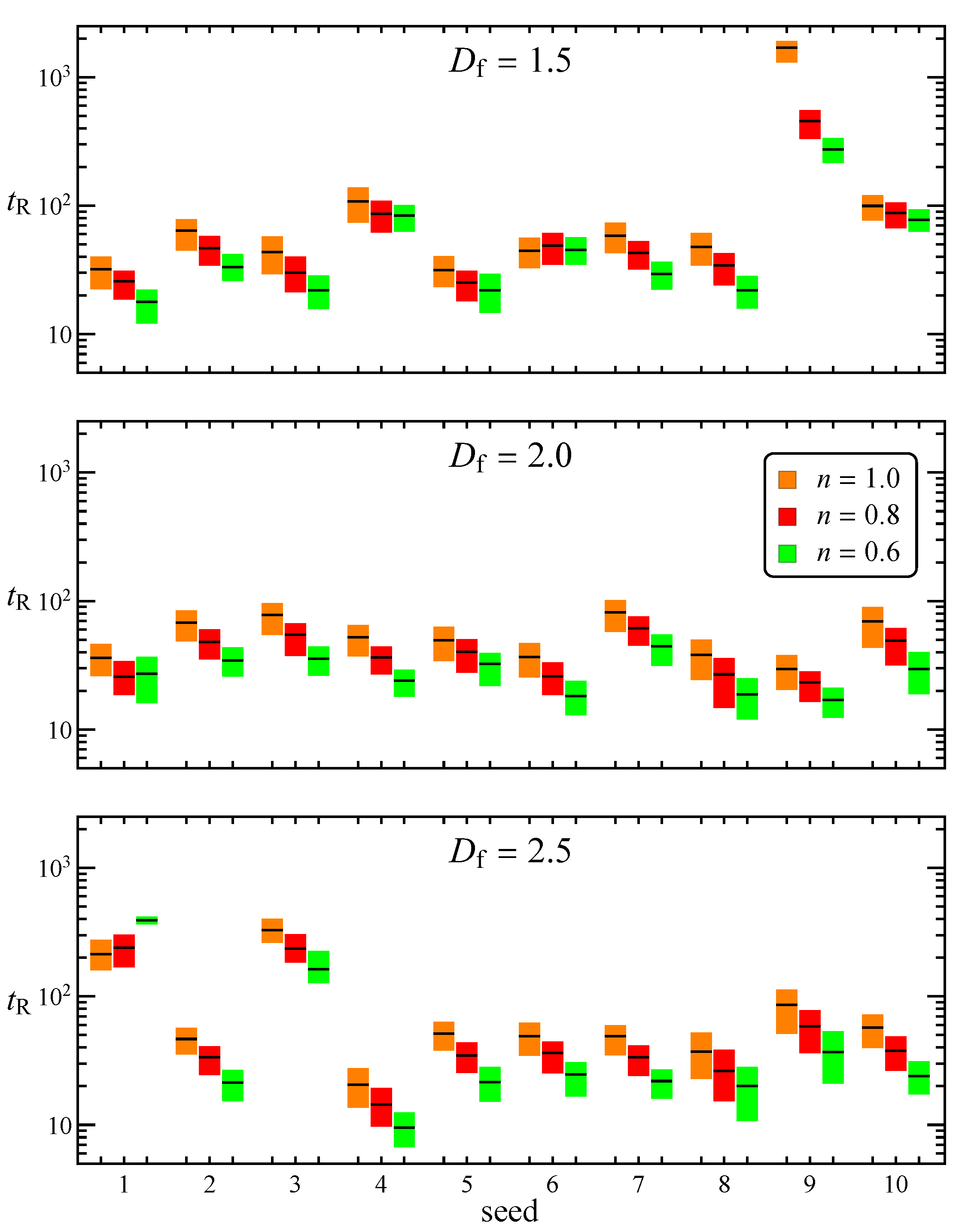
A relevant quantity for the sedimentation process is the time $t_{\mathrm{R}}$ needed to achieve the final regime. For instance, with reference to Figure 5, this is the time needed to travel along the orbits from the initial orientation to the green circle. Of course, the time strongly depends on the initial orientation. Thus, we compute the orbits followed by the aggregate with orientation starting from the 162 vertices of the spherical triangle mesh discussed in the previous section and, for each orbit, we estimate the time needed to achieve the regime within a certain tolerance. In case a single steady-state regime exists, we calculate the time the force requires to align with the equilibrium orientation within an angle tolerance of $5^{\circ }$. The results for $N_{\mathrm{p}}=20$ and different values of the seed, fractal dimension, and flow index are shown as box plots in Figure 7. The lower and higher limits of each box plot represent the first and third quartile over the different initial orientations, whereas the black dash is the median. In general, the (dimensionless) time decreases as the flow index decreases, whereas it is rather unaffected by the fractal dimension, ranging between 10 and 100 for almost all the examined cases. There are, however, some exceptions leading to remarkably longer times.

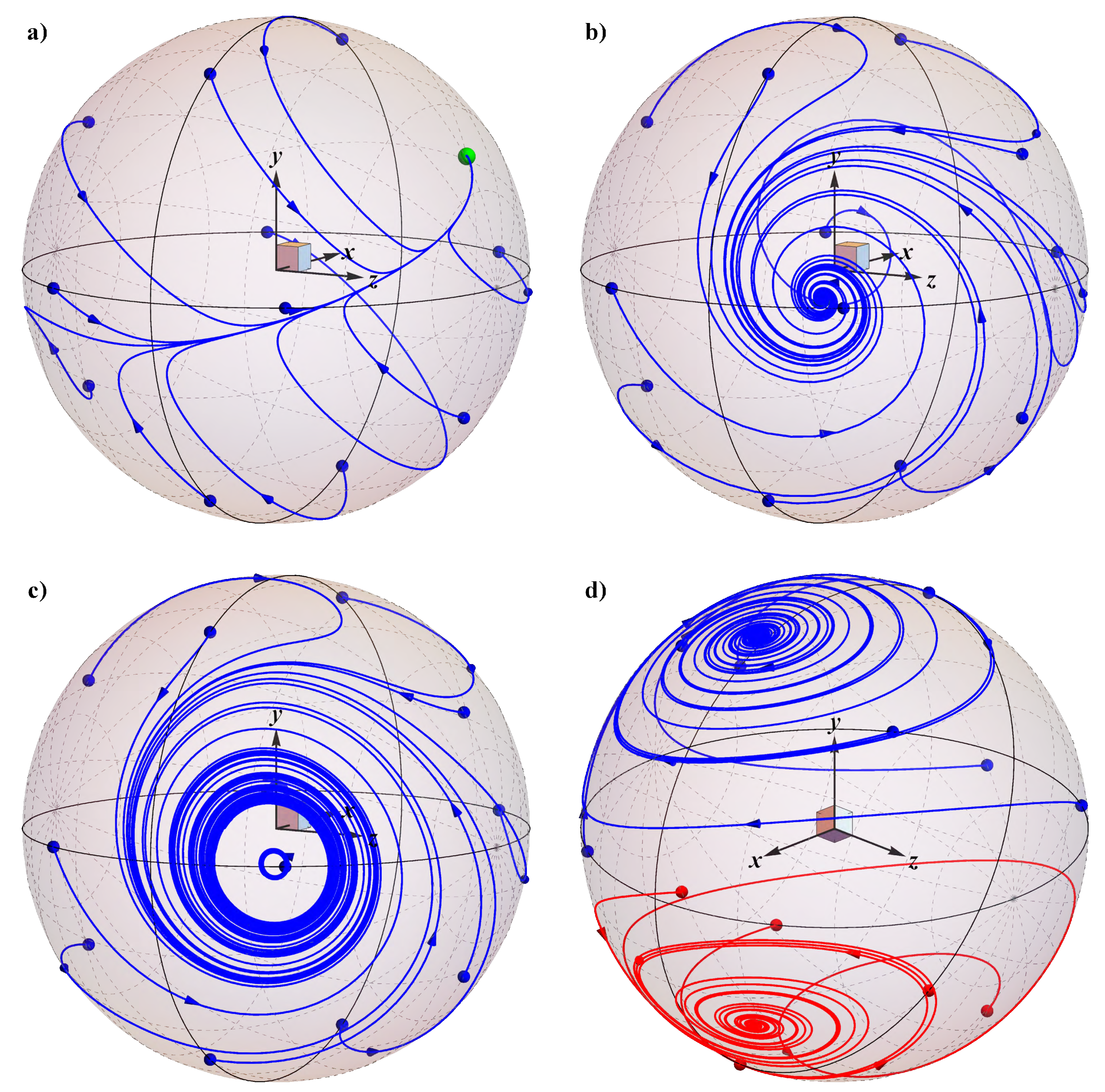
To investigate these particular cases more in detail, we show in Figure 8 the orbits described by the orientation of the force for (i) $n=1$, $D_{\mathrm{f}}=1.5$, $\mathrm{seed}=9$ (Figure 8a corresponding to the highest box plot in the top panel of Figure 7); (ii) $n=0.8$, $D_{\mathrm{f}}=2.5$, $\mathrm{seed}=1$ (Figure 8b corresponding to the leftmost red box plot in the bottom panel of Figure 7); and (iii) $n=0.6$, $D_{\mathrm{f}}=2.5$, $\mathrm{seed}=1$ (Figure 8c corresponding to the leftmost green box plot in the bottom panel of Figure 7). In the first case, we still observe a dynamics similar to what reported in Figure 5 with all the orbits converging to a single equilibrium point. However, at variance with the previous cases where the orbits independently moved towards the equilibrium point, now each trajectory converges first towards a common orbit and then, very slowly, to the equilibrium orientation, resulting in a drastic increase of the time needed to reach the steady-state regime. A similar dynamics is also observed for the same seed and for $n=0.8$ (red box plot) and $n=0.6$ (green box plot), as well as for $D_{\mathrm{f}}=2.5$ and $\mathrm{seed}=3$. A different scenario is observed for the second case (Figure 8b), where the orientation of the force follows spiraling trajectories before reaching the equilibrium point, also resulting in a longer transient dynamics. In the third case reported in Figure 8c, the regime becomes periodic with the presence of a limit cycle. Therefore, while settling, the aggregate continuously changes its orientation around the applied force, coming back to the same configuration after a certain period. Notice that the cases in Figure 8b,c correspond to the same aggregate (the fractal parameters and the seed are the same) and differ for the flow index. Further, the same aggregate in a Newtonian fluid ($n=1$) gives orbits like the ones shown in Figure 5. Thus, we conclude that, for this aggregate shape, a decrease of the flow index leads to the appearance of a bifurcation (specifically a Hopf bifurcation [44]) with a qualitative change in the regime attained by the aggregate. In the case of a periodic regime, the time reported in Figure 7 is evaluated as the time needed to reach the limit cycle within a tolerance of $5\%$ on X. Notice that the appearance of the bifurcation inverts the trend of $t_{\mathrm{R}}$ with the flow index (the values of the box plots corresponding to $\mathrm{seed}=1$ in Figure 7c increase with decreasing n). As the number of primary particles of the aggregate increases, another possible scenario, depicted in Figure 8d for $N_{\mathrm{p}}=50$, $D_{\mathrm{f}}=1.5$, $n=0.6$, appears. Two equilibrium regimes are observed, identified by the blue and red orbits. Therefore, depending on the initial configuration, the aggregate can orient along one of the two stable orientations.

By increasing the complexity of the shape, i.e., by increasing $N_{\mathrm{p}}$ and decreasing $D_{\mathrm{f}}$, spiraling orbits, periodic, and bistable regimes are more frequent, leading to a substantial increase of the time needed to reach the final orientation, and, more importantly, to a significant effect of the detailed morphology (i.e., the seed used to generate the aggregate) on the settling dynamics. This is illustrated in the middle and right panels of Figure 6 where the regime drag correction coefficient is shown as a function of the seed for $N_{\mathrm{p}}=50$ and $N_{\mathrm{p}}=100$. The periodic regime is denoted by two open squares identifying the maximum and minimum values of the oscillation, with a corresponding $X_{\mathrm{R}}$ calculated by averaging X over a period. The bistability is indicated by two closed circles that represent the values of $X_{\mathrm{R}}$ for the two equilibrium points. In Figure 6, the average of the regime drag correction coefficient over all the initial orientations ($\langle X_{\mathrm{R}}\rangle$ in Equation (13)) is also reported as a black dash. In case of a single equilibrium orientation, the unique solid circle coincides, in fact, with the dash. When multiple regimes coexist, the black dash is closer to the one that attracts more orbits. Notice that, in some cases (see, e.g., $N_{\mathrm{p}}=50$, $D_{\mathrm{f}}=1.5$, $\mathrm{seed}=9$, and $n=0.6$), the values of $X_{\mathrm{R}}$ for the two equilibrium points are remarkably different, resulting in a relevant quantitative effect of the initial orientation on the terminal velocity. At variance with the case at $N_{\mathrm{p}}=20$, the effect of the microstructure (seed) is much more relevant, leading to deviations up to $25\%$ from the value of the drag correction coefficient averaged over the seeds. In particular, maximum deviations are found for more elongated aggregates rather than sphere-like shapes. (Indeed, in the limiting case of a spherical aggregate, different seeds would produce the same shape.)

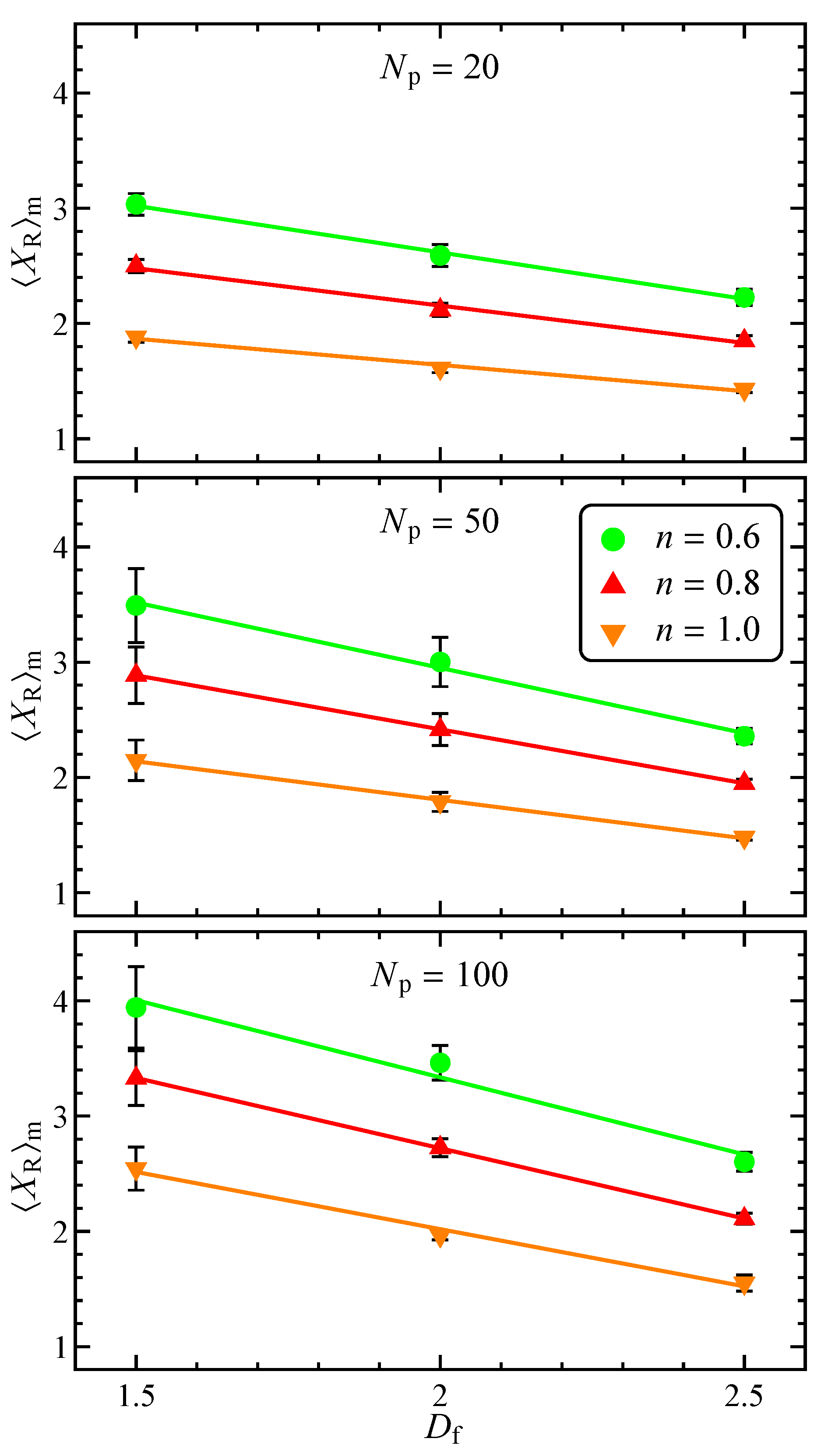
By averaging the data in Figure 6 over the seeds, we obtain the ensemble-average drag correction coefficient ${\langle X_{\mathrm{R}}\rangle }_{\mathrm{m}}$ reported in Figure 9. The data are shown as a function of the fractal dimension, where each panel refers to a fixed number of primary particles and the curves are parametric in the flow index. 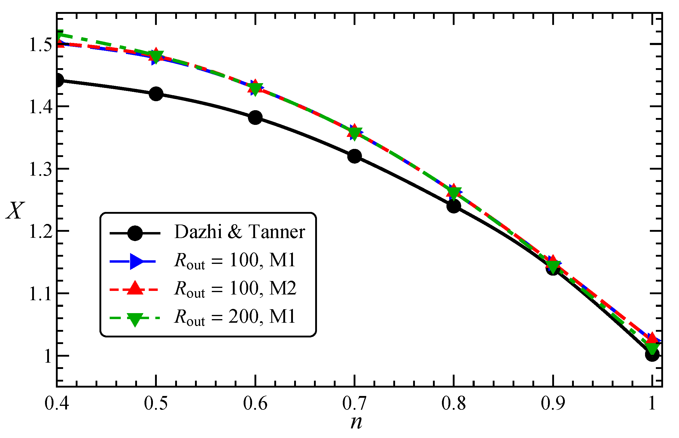For the Newtonian case (orange symbols), ${\langle X_{\mathrm{R}}\rangle }_{\mathrm{m}}$ can be used to calculate the hydrodynamic radius, which is found to be quantitatively consistent with the one reported in [33]. In the investigated range of $D_{\mathrm{f}}$, the drag correction factor is a linear decreasing function of the fractal dimension, i.e., an aggregate with a more spherical shape sediments faster than one with a rod-like morphology. In agreement with previous results for spheres [25], shear-thinning increases the drag correction coefficient. As already noted in Figure 6, higher values of ${\langle X_{\mathrm{R}}\rangle }_{\mathrm{m}}$ are observed as $N_{\mathrm{p}}$ increases. This effect is more evident for low fractal dimensions where a variation of the number of primary particles affects the aspect ratio of the aggregate, in turn altering the drag experienced by the particle. On the contrary, as previously remarked, for aggregates with a sphere-like shape (high $D_{\mathrm{f}}$), the number of primary particles mainly affects the “resolution” of the microstructure, without substantially changing the main geometrical features. For the same reason, the error bars are larger for low $D_{\mathrm{f}}$ and high $N_{\mathrm{p}}$. As a final note, we recall that, especially for low fractal dimension, a variation of the number of particles and flow index may lead to different dynamics followed by the aggregate while sedimenting. In some cases, our simulations evidenced a qualitative change of the regime attained by the particle (e.g., a bifurcation) as one of these parameters is varied, with obvious consequences on the drag correction factor and on the time needed to achieve such regime. These observations prevent us to derive a simple scaling of ${\langle X_{\mathrm{R}}\rangle }_{\mathrm{m}}$ with $N_{\mathrm{p}}$ and n. In this regard, also the averaging of $\langle X_{\mathrm{R}}\rangle$ over different seeds is, in some sense, misleading as it combines drag correction coefficients of aggregates that can experience very different dynamics. Therefore, we point out once again the importance of considering the detailed microstructure of the aggregate to correctly predict its sedimentation dynamics.

4. Conclusions

In this work, the hydrodynamic drag experienced by a fractal aggregate suspended in a non-Newtonian fluid is studied by numerical simulations. The aggregate shape is generated through a particle–cluster method combining equally-sized spherical particles. The power-law constitutive equation is used to model the suspending fluid. Finite element simulations are employed to solve the fluid dynamics governing equations, for orientations of the applied force uniformly distributed over the unit sphere. These velocities are interpolated and used to reconstruct the translational and orientational aggregate dynamics. The drag correction coefficient at long times is averaged over several initial orientations and particle shapes with the same fractal parameters.

The results show a relevant effect of the aggregate morphology and shear-thinning on the sedimentation dynamics. Depending on the fractal dimension, the number of primary particles forming the aggregate, and the flow index, the aggregate can undergo a variety of rotational dynamics while settling. These can lead to a stable orientation, periodic oscillations around the force direction, or coexistence of multiple equilibrium orientations, with relevant implications on the terminal velocity and the time needed to achieve the long-time regime.

The ensemble-average drag correction coefficient linearly decreases by increasing the fractal dimension in the investigated range, i.e., rod-like aggregates sediment more slowly than particles with an isotropic shape. Shear-thinning further reduces the settling velocity. At low fractal dimensions, the number of primary spheres has a relevant influence on the drag correction coefficient as it affects the aggregate aspect ratio. On the contrary, a weak effect is observed for aggregates with a sphere-like shape as an increase of the number of spheres does not produce a relevant change of the overall morphology.

The results reported in the present work highlight that the detailed particle shape needs to be considered to properly predict the sedimentation dynamics. As a matter of fact, a variation of the morphology, even with the same fractal characteristics, may lead to different transients and final regimes. Therefore, to properly understand the settling phenomenon, the connection between the shape of the aggregate and the resulting translational and rotational dynamics needs to be investigated. This will be the subject of future works.

Finally, we would like to point out that the present results, although discussed in the context of the sedimentation process, apply to any system in which a particle of fractal shape moves in a shear-thinning liquid in a uniform flow field. Indeed, regardless of the nature of the applied force, the particle experiences an hydrodynamic resistance that can be predicted from the results reported in this work. In this regard, neglecting the details of the specific morphology, our calculation can be exploited to derive a drag correlation model to be included in a computational fluid dynamic solver for simulating particle laden flows [45].

References

1. Bratby, J. Coagulation and Flocculation in Water and Wastewater Treatment; IWA Publishing: London, UK, 2016. [Google Scholar]
2. Stuetz, R.; Stephenson, T. Principles of Water and Wastewater Treatment Processes; IWA Publishing: London, UK, 2009. [Google Scholar]
3. Spicer, P.T.; Pratsinis, S.E. Shear-induced flocculation: The evolution of floc structure and the shape of the size distribution at steady state. Water Res. 1996, 30, 1049–1056. [Google Scholar] [CrossRef]
4. Gregory, J. Monitoring particle aggregation processes. Adv. Colloid Interface Sci. 2009, 147–148, 109–123. [Google Scholar] [CrossRef] [PubMed]
5. He, W.; Nan, J.; Li, H.; Li, S. Characteristic analysis on temporal evolution of floc size and structure in low-shear flow. Water Res. 2012, 46, 509–520. [Google Scholar] [CrossRef] [PubMed]
6. Moruzzi, R.B.; de Oliveira, A.L.; da Conceição, F.T.; Gregory, J.; Campos, L.C. Fractal dimension of large aggregates under different flocculation conditions. Sci. Total Environ. 2017, 609, 807–814. [Google Scholar] [CrossRef] [Green Version]
7. Oh, C.; Sorensen, C. The Effect of Overlap between Monomers on the Determination of Fractal Cluster Morphology. J. Colloid Interface Sci. 1997, 193, 17–25. [Google Scholar] [CrossRef] [PubMed]
8. Melas, A.D.; Isella, L.; Konstandopoulos, A.G.; Drossinos, Y. Morphology and mobility of synthetic colloidal aggregates. J. Colloid Interface Sci. 2014, 417, 27–36. [Google Scholar] [CrossRef] [PubMed] [Green Version]
9. Johnson, C.P.; Li, X.; Logan, B.E. Settling Velocities of Fractal Aggregates. Environ. Sci. Technol. 1996, 30, 1911–1918. [Google Scholar] [CrossRef]
10. Vahedi, A.; Gorczyca, B. Predicting the settling velocity of flocs formed in water treatment using multiple fractal dimensions. Water Res. 2012, 46, 4188–4194. [Google Scholar] [CrossRef]
11. Durlofsky, L.; Brady, J.F.; Bossis, G. Dynamic simulation of hydrodynamically interacting particles. J. Fluid Mech. 1987, 180, 21. [Google Scholar] [CrossRef] [Green Version]
12. Hassonjee, Q.; Ganatos, P.; Pfeffer, R. A strong-interaction theory for the motion of arbitrary three-dimensional clusters of spherical particles at low Reynolds number. J. Fluid Mech. 1988, 197, 1–37. [Google Scholar] [CrossRef] [Green Version]
13. Filippov, A. Drag and Torque on Clusters of N Arbitrary Spheres at Low Reynolds Number. J. Colloid Interface Sci. 2000, 229, 184–195. [Google Scholar] [CrossRef] [PubMed]
14. Binder, C.; Feichtinger, C.; Schmid, H.J.; Thürey, N.; Peukert, W.; Rüde, U. Simulation of the hydrodynamic drag of aggregated particles. J. Colloid Interface Sci. 2006, 301, 155–167. [Google Scholar] [CrossRef] [PubMed]
15. Chopard, B.; Nguyen, H.; Stoll, S. A lattice Boltzmann study of the hydrodynamic properties of 3D fractal aggregates. Math. Comput. Simul 2006, 72, 103–107. [Google Scholar] [CrossRef]
16. Schlauch, E.; Ernst, M.; Seto, R.; Briesen, H.; Sommerfeld, M.; Behr, M. Comparison of three simulation methods for colloidal aggregates in Stokes flow: Finite elements, lattice Boltzmann and Stokesian dynamics. Comput. Fluids 2013, 86, 199–209. [Google Scholar] [CrossRef]
17. Happel, J.; Brenner, H. Low Reynolds Number Hydrodynamics: With Special Applications to Particulate Media; Springer: Dordrecht, The Netherlands, 1981. [Google Scholar]
18. Kim, A.S.; Stolzenbach, K.D. The Permeability of Synthetic Fractal Aggregates with Realistic Three-Dimensional Structure. J. Colloid Interface Sci. 2002, 253, 315–328. [Google Scholar] [CrossRef] [Green Version]
19. Fellay, L.S.; Twist, C.; Vanni, M. Motion of rigid aggregates under different flow conditions. Acta Mech. 2013, 224, 2225–2248. [Google Scholar] [CrossRef]
20. Harshe, Y.M.; Ehrl, L.; Lattuada, M. Hydrodynamic properties of rigid fractal aggregates of arbitrary morphology. J. Colloid Interface Sci. 2010, 352, 87–98. [Google Scholar] [CrossRef]
21. Seyssiecq, I.; Ferrasse, J.H.; Roche, N. State-of-the-art: Rheological characterisation of wastewater treatment sludge. Biochem. Eng. J. 2003, 16, 41–56. [Google Scholar] [CrossRef]
22. Ratkovich, N.; Horn, W.; Helmus, F.; Rosenberger, S.; Naessens, W.; Nopens, I.; Bentzen, T. Activated sludge rheology: A critical review on data collection and modelling. Water Res. 2013, 47, 463–482. [Google Scholar] [CrossRef]
23. Wasserman, M.L.; Slattery, J.C. Upper and lower bounds on the drag coefficient of a sphere in a power-model fluid. AIChE J. 1964, 10, 383–388. [Google Scholar] [CrossRef]
24. Chhabra, R.P.; Uhlherr, P.H.T. Creeping motion of spheres through shear-thinning elastic fluids described by the Carreau viscosity equation. Rheol. Acta 1980, 19, 187–195. [Google Scholar] [CrossRef]
25. Dazhi, G.; Tanner, R. The drag on a sphere in a power-law fluid. J. Non-Newton. Fluid Mech. 1985, 17, 1–12. [Google Scholar] [CrossRef]
26. Chhabra, R.P. Bubbles, Drops, and Particles in Non-Newtonian Fluids; Taylor & Francis Inc.: Boca Raton, FL, USA, 2006. [Google Scholar]
27. Tripathi, A.; Chhabra, R.P.; Sundararajan, T. Power law fluid flow over spheroidal particles. Ind. Eng. Chem. Res. 1994, 33, 403–410. [Google Scholar] [CrossRef]
28. Thouy, R.; Jullien, R. A cluster–cluster aggregation model with tunable fractal dimension. J. Phys. A Math. Gen. 1994, 27, 2953–2963. [Google Scholar] [CrossRef]
29. Meakin, P. A Historical Introduction to Computer Models for Fractal Aggregates. J. Sol-Gel Sci. Technol. 1999, 15, 97–117. [Google Scholar] [CrossRef]
30. Vormoor, O. Large scale fractal aggregates using the tunable dimension cluster–cluster aggregation. Comput. Phys. Commun. 2002, 144, 121–129. [Google Scholar] [CrossRef]
31. Brown, M.; Errington, R.; Rees, P.; Williams, P.; Wilks, S. A highly efficient algorithm for the generation of random fractal aggregates. Phys. D 2010, 239, 1061–1066. [Google Scholar] [CrossRef]
32. Mroczka, J.; Woźniak, M.; Onofri, F.R. Algorithms and methods for analysis of the optical structure factor of fractal aggregates. Metrol. Meas. Syst. 2012, 19, 459–470. [Google Scholar] [CrossRef] [Green Version]
33. Filippov, A.; Zurita, M.; Rosner, D. Fractal-like Aggregates: Relation between Morphology and Physical Properties. J. Colloid Interface Sci. 2000, 229, 261–273. [Google Scholar] [CrossRef]
34. Skorupski, K.; Mroczka, J.; Wriedt, T.; Riefler, N. A fast and accurate implementation of tunable algorithms used for generation of fractal-like aggregate models. Phys. A 2014, 404, 106–117. [Google Scholar] [CrossRef]
35. Trofa, M.; D’Avino, G.; Maffettone, P.L. Numerical simulations of a stick-slip spherical particle in Poiseuille flow. Phys. Fluids 2019, 31, 083603. [Google Scholar] [CrossRef]
36. Trofa, M.; D’Avino, G. Rheology of a Dilute Suspension of Aggregates in Shear-Thinning Fluids. Micromachines 2020, 11, 443. [Google Scholar] [CrossRef]
37. Lawson, C.L. C1 surface interpolation for scattered data on a sphere. Rocky Mt. J. Math. 1984, 14, 177–202. [Google Scholar] [CrossRef]
38. Carfora, M.F. Interpolation on spherical geodesic grids: A comparative study. J. Comput. Appl. Math. 2007, 210, 99–105. [Google Scholar] [CrossRef] [Green Version]
39. Rapaport, D.C. The Art of Molecular Dynamics Simulation; Cambridge University Press: Cambridge, UK, 2004. [Google Scholar]
40. Hu, H.H.; Patankar, N.; Zhu, M. Direct Numerical Simulations of Fluid–Solid Systems Using the Arbitrary Lagrangian–Eulerian Technique. J. Comput. Phys. 2001, 169, 427–462. [Google Scholar] [CrossRef]
41. D’Avino, G.; Maffettone, P.; Greco, F.; Hulsen, M. Viscoelasticity-induced migration of a rigid sphere in confined shear flow. J. Non-Newton. Fluid Mech. 2010, 165, 466–474. [Google Scholar] [CrossRef]
42. Zhou, Q. PyMesh–Geometry Processing Library for Python. 2018. Available online: https://github.com/qnzhou/PyMesh (accessed on 10 April 2020).
43. Geuzaine, C.; Remacle, J.F. Gmsh: A 3-D finite element mesh generator with built-in pre- and post-processing facilities. Int. J. Numer. Methods Eng. 2009, 79, 1309–1331. [Google Scholar] [CrossRef]
44. Strogatz, S. Nonlinear Dynamics and Chaos: With Applications to Physics, Biology, Chemistry, and Engineering; Westview Press: Boulder, CO, USA, 2015. [Google Scholar]
45. Zhou, Z.; Kuang, S.; Chu, K.; Yu, A. Discrete particle simulation of particle–fluid flow: Model formulations and their applicability. J. Fluid Mech. 2010, 661, 482–510. [Google Scholar] [CrossRef]
Figure 1. Examples of aggregate shapes obtained from the particle–cluster method for N p = 20 , k f = 1.3 , and D f = 1.5 (a), and D f = 2.5 (b). To avoid numerical issues due to the tangent point, the centers of the spheres in contact are connected with a set of cylinders with radius 0.732 a . In panels (c,d), the final geometry of the aggregates and the surface mesh are shown. The computational domain and the mesh on the external spherical surface is displayed in panel (e).
Applsci 10 03267 g001
Figure 2. Drag correction coefficient X as a function of the flow index n for a spherical particle in an unbounded power-law fluid. The black circles are the simulation results by Dazhi and Tanner [25], and the triangles are obtained by our simulations for different mesh resolutions and size of the external domain.
Applsci 10 03267 g002
Figure 3. (ac) Drag correction coefficient for the aggregate shown in Figure 1a ( N p = 20 , D f = 1.5 ) as a function of the force direction identified by the spherical coordinates ( θ , ϕ ) for the Newtonian fluid (a), the power-law fluid with n = 0.8 (b), and n = 0.6 (c). (d) Dimensionless area projected along the direction of the applied force for the same aggregate as in panels (ac). The symbols denote the direction of the force attained at long times for the Newtonian fluid (circle), power-law fluid with n = 0.8 (square) and n = 0.6 (triangle).
Applsci 10 03267 g003
Figure 4. (ac) Drag correction coefficient for the aggregate shown in Figure 1b ( N p = 20 , D f = 2.5 ) as a function of the force direction identified by the spherical coordinates ( θ , ϕ ) for the Newtonian fluid (a), the power-law fluid with n = 0.8 (b), and n = 0.6 (c). (d) Dimensionless area projected along the direction of the applied force for the same aggregate as in panels (ac). The symbols denote the direction of the force attained at long times for the Newtonian fluid (circle), power-law fluid with n = 0.8 (square) and n = 0.6 (triangle).
Applsci 10 03267 g004
Figure 5. Orbits described by the orientation of the applied force for 12 initial orientations (blue circles) uniformly distributed over the unit sphere for: the aggregate shown in Figure 1a ( N p = 20 , D f = 1.5 ) in a Newtonian (a) or power-law fluid with n = 0.6 (b), the aggregate shown in Figure 1b ( N p = 20 , D f = 2.5 ) in a Newtonian (c) or power-law fluid with n = 0.6 (d). The equilibrium points are denoted by green circles.
Applsci 10 03267 g005
Figure 6. Regime drag correction coefficient X R and its average over the initial orientations X R for different number of primary particles (columns), fractal dimension (rows), random seed for the aggregate generation (bands), and flow index (orange n = 1 , red n = 0.8 , and green n = 0.6 ). Solid circles and open squares denote steady-state and periodic regimes. The black dashes represent X R .
Applsci 10 03267 g006
Figure 7. Box plot of the times needed for an aggregate to reach a stable regime as a function of particle random seed, flow index, and fractal dimension. The number of primary particles is N p = 20 . The black dash within each box represents the median of the distribution.
Applsci 10 03267 g007
Figure 8. Orbits described by the orientation of the applied force for 12 initial orientations (blue circles) uniformly distributed over the unit sphere. The parameters are (a) n = 1 , N p = 20 , D f = 1.5 , seed = 9 ; (b) n = 0.8 , N p = 20 , D f = 2.5 , seed = 1 ; (c) n = 0.6 , N p = 20 , D f = 2.5 , seed = 1 ; (d) n = 0.6 , N p = 50 , D f = 1.5 , seed = 9 .
Applsci 10 03267 g008
Figure 9. Ensemble-average drag correction coefficient as a function of fractal dimension, parametric in the number of aggregate primary particles and for different flow indexes. The data standard deviation and trend line are also reported.
Applsci 10 03267 g009