1. Introduction
Design of engineering structures is carried out in a way to ensure safety of occupants during their service life while reducing cost and at the same time maintaining quality. Failure to do so may lead to catastrophic human losses and necessitate heavy capital expenditure or expensive maintenance repair. Hence, it is important to monitor changes in the structural parameters such as stiffness, damping, and mass. Structural health monitoring (SHM) is an emerging technology to detect damage in structure and to identify potential deficiency states at an early stage by examining sensors data mounted on structures or other sensing devices [
1]. Vibration-based damage detection (VDD) is the dominant technique for a robust damage detection that uses the changes in dynamic parameters of structures for finding indications of damages [
2,
3].
Establishing calculation model and identifying dynamic parameters of a vibrating system is the key issue to these methods [
4,
5]. VDD has been subject of extensive research in recent years due to accurate results and the reliable damage identification [
6,
7,
8]. Fan and Qiao [
9] conducted a comprehensive review on modal parameter based VDD methods. It was stated that in these VDD methods, damage can be identified by variation in natural frequency, mode shape, curvature mode shape, and both frequencies and mode shapes. The potential and drawbacks of each method is discussed. It is stated that natural frequency is suitable for damage detection whereas mode shape and curvature mode shape is generally used for damage localization. Moughty and Casas [
10] provided a review of current developments in VDD techniques for small to medium span bridges. It was determined that output-only approaches that use non-modal models offer significant advantage due to ease of application, higher sensitivity and robustness. Das et al. [
11] conducted a comparative study to evaluate different VDD methods. In the paper four different categories of VDD methods including local diagnostic fundamental modal examination, non-probabilistic, and time domain methods were compared. It was stated that time-domain methods proved more successful damage identification than the rest of the methods. Reynders [
12] provided a comprehensive review on operational modal analysis using vibration response of structures. In the study the system identification methods are revealed. Then, some powerful system identification algorithms are discussed and different algorithms and approaches are compared. Moreover, Stochino et al. [
13] discussed about economic aspect of VDD using a bridge case study.
System identification methods provide a powerful tool to construct analytical model of a dynamic system [
14]. These methods rely on the hypothesis that changes in physical parameters of a structure changes its dynamic behavior [
15,
16]. System identification is one the powerful methods to extract dynamic parameters of structures. These methods utilize approximate solutions for estimating system parameters and for exploiting possible damage-related variations in structures [
17,
18].
Based on the used measurement data system identification methods can be categorized into two input-output and output-only classes [
5,
19]. Output-only methods use the structural response of operational and environmental excitation forces for identification of system parameters. Output-only methods are more favorable choice due to ease of setup less-intrusive nature, and lower maintenance cost [
6]. Acceleration, velocity and displacement signals are the measures that can be used for system identification in vibrating structures [
20]. However, acceleration response is the most frequently used measure for VDD due to relatively superior signal-to-noise ratio at high spectral range, high sensitivity, cost-effectiveness of acceleration transducers, and Installation convenience of acceleration transducers [
20,
21]. Several studies have used acceleration response as their input data which among them Kordestani and Zhang [
22], Kordestani et al. [
23], and Rashidi et al., [
24] can be mentioned. Xin et al. [
25] studied the performance of input-output and output-only algorithms in an offshore platform under three different excitation signals of step relaxation, impact, and ground motion. All procedures had good agreement with estimated modal frequencies of stronger modes.
In a pioneering work, Overschee et al. [
26] introduced stochastic subspace identification (SSI) together with combined and deterministic models within a unified framework. Due to the direct use of the response data in identification process, the method was named data-driven stochastic subspace identification or SSI-DATA. SSI-DATA is a numerically robust algorithm that uses QR decomposition to project future data on the past subspace [
27]. The proposed stochastic subspace method use Hankel block matrix of the output data to analyze system and extract the state space model. The proposed algorithm has been broadly approved and has been extensively applied for identification of the system parameters particularly in the SHM. Peeters and De Roeck [
28] introduced applied SSI in SHM. Döhler and Mevel [
29] proposed using a fast SSI scheme to solve the least squares problems. Döhler and Mevel [
30] defined an robust SSI algorithm by potential capability of rejecting uncertainty of systems. Cho et al. [
31] used a decentralized SSI algorithm for wireless sensor networks (WSNs). Dai et al. [
32] modified Hankel matrix by adding harmonic vectors to modify modal identification of harmonic excited structures with close natural frequencies.
Van Overschee et al. [
26] extended the concept of weight matrices as a basis for the column space of the extended observability matrix in subspace algorithm. Three different implementations for SSI were introduced that included: Unweighted principal component (UPC), principal component (PC), and canonical variate analysis (CVA). Though the most studies in the field of SSI use the fundamentals of the algorithm developed by Van Overschee et al. [
26] in their analysis, the incorporated weight matrices in the identification process is not clearly demonstrated [
33,
34,
35].
PC algorithm simplifies data by orthogonal transformation of observations to a set of independent variables termed as principal variables. The first principal components of this transformation have higher variance. CVA is a linear regression to quantify a relation between a normalized and expectation variable. UPC is the simplest of three SSI algorithms that considers unit weight matrices for both. Only a limited number of studies are available that compare the performance of weight matrices of PC, CVA, or UPC for system identification. However, the findings not only do not support each, other but also contradict each other in some cases. Alam et al. [
36] used SSI for modal testing of on-orbit space satellite appendage. The results show that PC approach was unable to estimate modal parameters. Identified mode shapes using UPC and CVA approaches match very well with simulation results. CVA had better performance for low order excited modes.
Kompalka et al. [
37] stipulated that different weighting matrices yield similar results for modal parameter identification. However, Nguyen [
38] and Cismaşiu et al. [
39] indicated that SSI-UPC had superior performance compared to other weight matrices for damage detection of structures. Pioldi et al. [
40] demonstrated that the CVA is the most stable weighting option in experimental modal analysis whereas Miguel et al. [
41] chosen the variant PC for system identification.
Several researchers have discussed about using different parameters of SSI algorithms in identification robustness, accuracy, and computation time. However, limited number of research has comprehensively investigated the impact of weight factors in identified system using SSI algorithm. Moreover, the obtained results in these studies do not support superior performance in any specific SSI methodologies or contradictory results are reported in some cases. The present study aimed at evaluating the effect of using weight matrices on efficiency of the identified system parameters. The current paper investigates the theory behind the PC, UPC, and CVA algorithms and presents different examples to evaluate the weight matrices. Three different indicators are introduced in the evaluation process that includes fit values analysis, poles estimation, and computation time. The results from several cases indicate that the UPC algorithm provides the best performance.
The paper is organized as follows:
Section 2 provides the methodology of the study and theory behind the design and implementation of the subspace algorithm. In
Section 3 and
Section 4, the numerical and experimental examples for verification of the weight matrices are presented, respectively. In
Section 5, the findings of the study are presented and discussed. Finally, concluding remarks of the work are given in
Section 6.
2. Methods
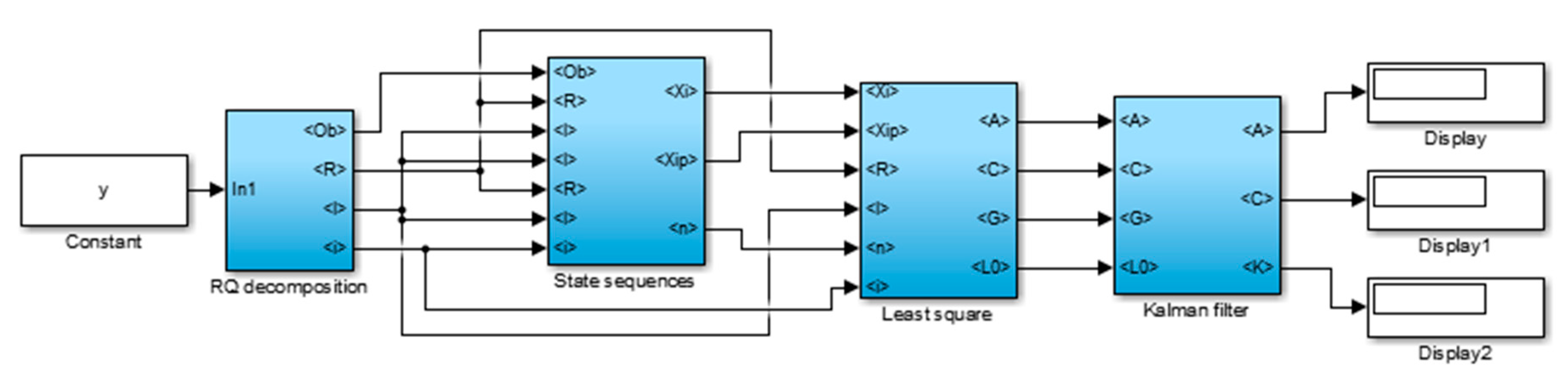
By assuming applied loads as an unmeasured white-noise signal, SSI can be defined as an output-only identification method. SSI-DATA algorithm consists of four main steps including:
State-space of a dynamic system is extracted from the product of extended observability matrix and state sequence. The appropriate order of a system is predicted using singular value decomposition (SVD). System order (number of modes) is the only user-defined parameter in subspace identification method and must be selected carefully to obtain meaningful results.
Figure 1 shows the configuration for implementation SSI-DATA.
2.1. RQ Decomposition
The output-only stochastic methods aim to estimate system matrices directly from measured acceleration response. To this end, output measurements are re-structured in order to construct Block Hankel matrix of SSI algorithm. Hankel matrix provides an enhanced form to take advantages of its appealing properties in linear algebra. Hankel matrix is a full-rank block matrix that transforms measurement row vector into block matrix which is identical along matrix’s anti-diagonals. Hankel matrix is partitioned into past and future input data as shown in Equation (1). It is efficient to set the size of Hankel matrix into columns where is number of rows and is number of columns.
In the first step, some characteristic values of extended observability matrix and system-order are calculated. For the second step, system matrices are calculated from the extracted observability matrix. Differences among subspace algorithms are in the way the system matrices are calculated from the observability matrices. In SS-DATA, first, state sequences are extracted from the extended observability matrix and then system matrices are derived solving a set of least squares equations [
42]. A unifying theorem is adapted to determine extended observability matrix and system-order by calculating oblique projection. The theorem is based on rearranging the extracted response measurements
data into Hankel block matrix.
where
and
subscripts, respectively, denote the past and future sequences of the output data.
RQ decomposition is used to calculate oblique projection of Hankel matrix. The resultant of
and
matrices are upper triangular and orthogonal matrices, respectively.
Since
is a triangular matrix the computational burden to estimate corresponding system matrices are dramatically reduced by using this decomposition technique.
where
and
are obtained by shifting the borders of the future and past data block down.
Principle angle and direction between two subspaces and can be determined using SVD. The cosines of the principle angles
are denoted by the singular values
.
where
and
are weighting matrices of the singular angles to estimate system order. The system order
is a vector formed by the diagonal elements of the singular value matrix. Three methods are defined for determination of the weighting matrices including:
Principle component (PC);
Unweighted principle component (UPC); and
Canonical variate analysis (CVA).
Assigning two weighting matrices of and allows to draw a proper state-space basis of an identified model. SVD is one of the most powerful matrix decomposition techniques from linear algebra. In the theory of SVD, any real-valued matrix of dimension could be decomposed into , where and are orthogonal matrices and is a diagonal matrix called the singular value. The SVD method is implemented to extract balanced realization using PC, UPC and CVA algorithms in SSI. The below provide an overview of each weighting method.
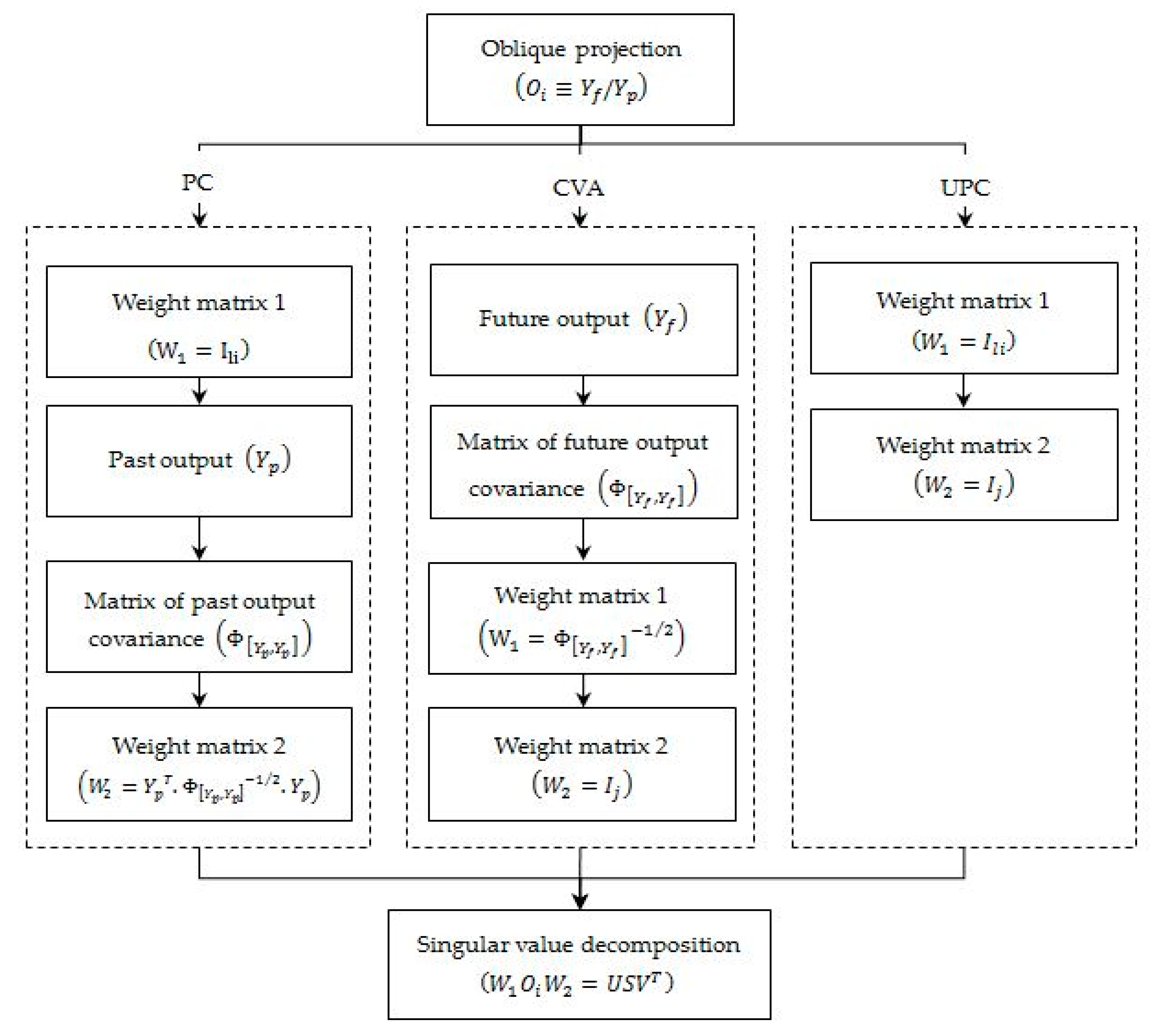
2.1.1. Principal Component (PC)
PC is one of the methods to determine weight matrix for SSI algorithm. PC algorithm incorporates a right weight matrix to calculate singular values. The block Toeplitz matrix is obtained using the output covariance matrix of the past and future data
. The principle components of the covariance Toeplitz matrix
are used for weighting of the estimated results.
The SVD of the estimated
matrix reveals system order, column range
and the row range
. A deterministic balanced realization of the state-space equation is achieved through using weighting matrices of
and
.
By using the left singular vectors and the singular values of the weighted projection, the extended observability matrix (and) could be determined as shown in Equations (13) and (14). Equation (14) presents how the extended observability matrix is used to calculate state parameters.
2.1.2. Unweighted Principal Component (UPC)
Unweighted principle component (UPC) method is considered as a special case of PC analysis. The UPC algorithm gives the first principle component index of a system and gives equal weight factors to each set of data. The UPC is the simplest version of SSI.
and
can be casted into the form of identity matrices in the framework of the UPC algorithm as shown in Equations (9) and (10).
The balanced realization is determined shifting the stochastic process into a deterministic forward innovation model. Left singular vector is used to determine the extended observability matrix in UPC.
2.1.3. Canonical Variate Algorithm (CVA)
CVA proposes selecting equal weight for all incorporated system modes extracted from excitation measurement data. The weighting matrices in CVA are obtained after applying SVD. It could be determined by choosing the following weights correspond to the canonical variate algorithm.
The weighting matrix
in CVA is chosen in a way that the diagonal of S matrix contains the cosines of the angle between principal subspaces of the system. The flowchart for calculation of PC, UPC and CVA weight matrices is shown in
Figure 2.
2.2. Estimation of the State Sequences
In order to eliminate dependence of the algorithm on future output data (
), the concept of geometrical projections of the future output onto the past output subspaces is deployed. The observability matrix of the system is obtained from:
The oblique projection
of the past and future output data are used to determine the state of a system
and to estimate the extended observability matrix
.
By shifting data sequences one step ahead, the oblique projection of
could be calculated. Multiplication of the pseudo-inverse of the extended observability matrix without the last block row
into the oblique projection results in the state sequence of the future data
.
As it can be seen in Equations (14) and (15), state sequence of Kalman filter is obtained directly from output data sequence without dependence on geometrical interpretation or priori knowledge of system matrices. In the next section the least square application to drive and matrices is discussed. The corresponding state sequences of and can be used to obtain the state-space representation of the system as shown in Equations (14) and (15).
2.3. Least Square Solution
Output-only stochastic method can be written in the form of state-space model. The matrix model of the state-space concept can be represented by Equation (16). Hence, the system matrices could be extracted directly using the output response of structure.
where
and
are zero mean, Gaussian white noise terms corresponding to the process and measurement noise, respectively. Using the least square (LS) method,
and
matrices were calculated in the previous section. Since the Kalman filter residuals of
and
are orthogonal and uncorrelated with the state sequence, Equation (16) could be written as:
In the next subsection, the transformation of the and matrices into forward innovation Kalman filter is presented.
2.4. Kalman Filter
Kalman filter has a key role in derivation of stochastic subspace algorithm. The estimated state sequence (
) of the system using non-steady Kalman filtr can be obtained through noise covariance. By solving the Lyapunov equation, the estimation value of the covariance matrices (
,
and
S) are inferred. Knowing the system matrices (
and
) and the noise (
and
) together with covariance matrices are the parameters required for Kalman filtering and
,
,
, and
could be simply derived.
A forward innovation model is introduced in the formula of the Riccati equation as shown in Equations (22) and (23). The Riccati equation is solved using Schur decomposition.
The Kalman filter gain
is obtained from Equation (23). The state-space model of the output-only dynamic system can be presented by:
The Kalman gain is estimated through the Kalman process to update the future data corresponding to a certain pattern, independent of the noise covariance data.
3. Numerical Case Study
The subspace method is adopted from [
26] and the weight matrices are introduced. The state-space equation of dynamic systems is extracted by using different weight matrices for each numerical and experimental case-study. Furthermore, separate evaluation algorithms are implemented for analysis of time-efficiency, noise-robustness, and accuracy. The algorithms include but are not limited to:
Identification of the system parameters using all three weight matrices;
Calculating pole values by solving the system’s characteristic equation;
Predicting the estimation value and comparison with the real signal response by calculation of the error residual, variance, and the associated variance accounted for (VAF);
Implementing fairly large number of identification cycles and measuring the elapsed time for every step; and
Plotting the obtained results for each algorithm.
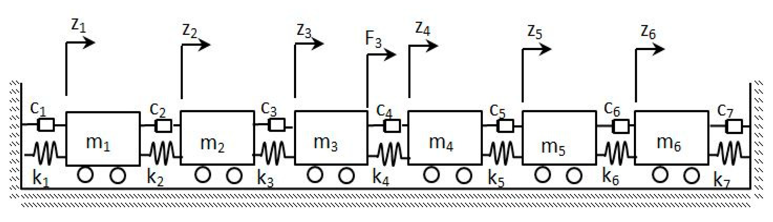
A 6-degree of freedom, lumped mass model is used as the numerical example to evaluate different subspace algorithms. The configuration of the simulation model is shown in
Figure 3.
The main parameters of the numerical example are as follows:
and
are damping stiffness and mass matrices, respectively. The stiffness equals to
N/m for each mass to mass interlink.
is an identity matrix of size six. Rayleigh damping coefficients are as:
equal to:
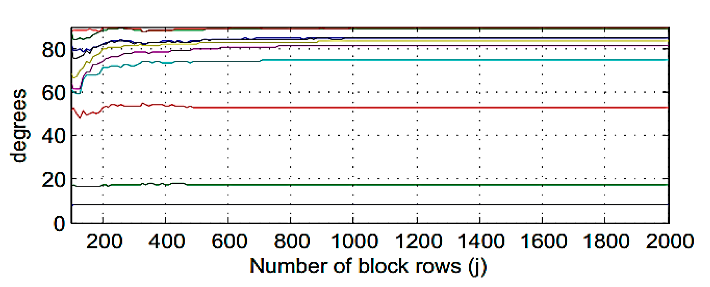
An impulsive load of 1 kN is applied to the dynamic model. The sampling frequency for obtained acceleration response is 500 Hz. Random noise with different ratios are induced to the response signal to simulate the applied ambient uncertainty. The ratio of the applied noise is demonstrated in each evaluation process. System order can be determined by inspecting convergence of the principal angles toward 90 degrees. In
Figure 4, the CVA principal angles are plotted versus the block rows. The convergence of the principal angles is achieved by increasing the number of block rows. The first iteration starts from nearly 10 degrees. Second and third iterations are around 20 and 50 degrees. It can be seen that the principal angles approach to 90 degrees after 10 iterations that means the optimum system order of 10 or above, can be selected to reach the optimum estimating of the simulation model.
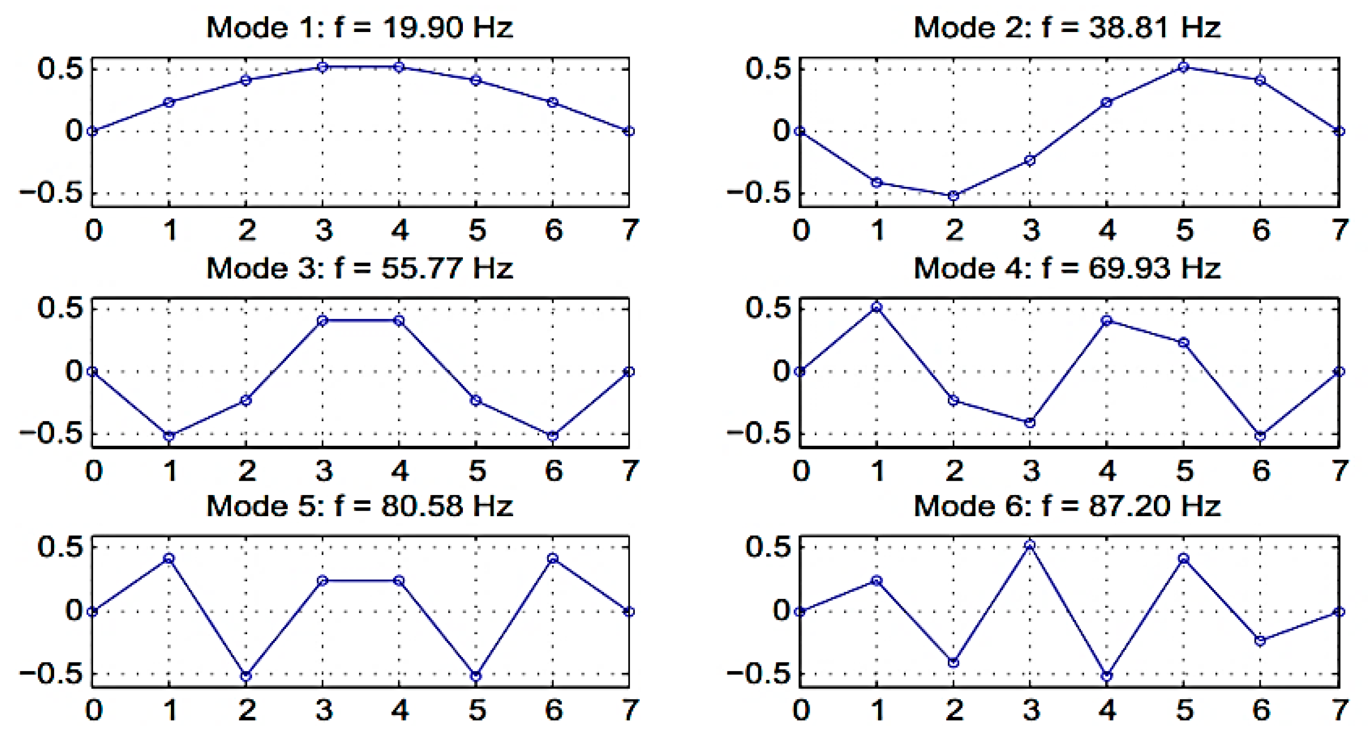
Poles of the simulation system are extracted from the system parameters of the SSI algorithm. The first natural frequencies and mode shapes of the simulation model with the assumption of zero damping are shown in
Figure 5. However, the eigensolution of the damped structures are in the form of complex dynamic parameters.
3.1. Estimation Accuracy
The estimation accuracy of SSI is demonstrated with similarity measure of VAF. VAF value is an indicator to quantify the relationship between the estimated and actual values of an obtained signal. Higher VAF values means that the estimates present a better fit into an existing signal, thus, better performance [
43]. VAF criterion is calculated from the variance of the estimation residual
on variance of the response signal
.
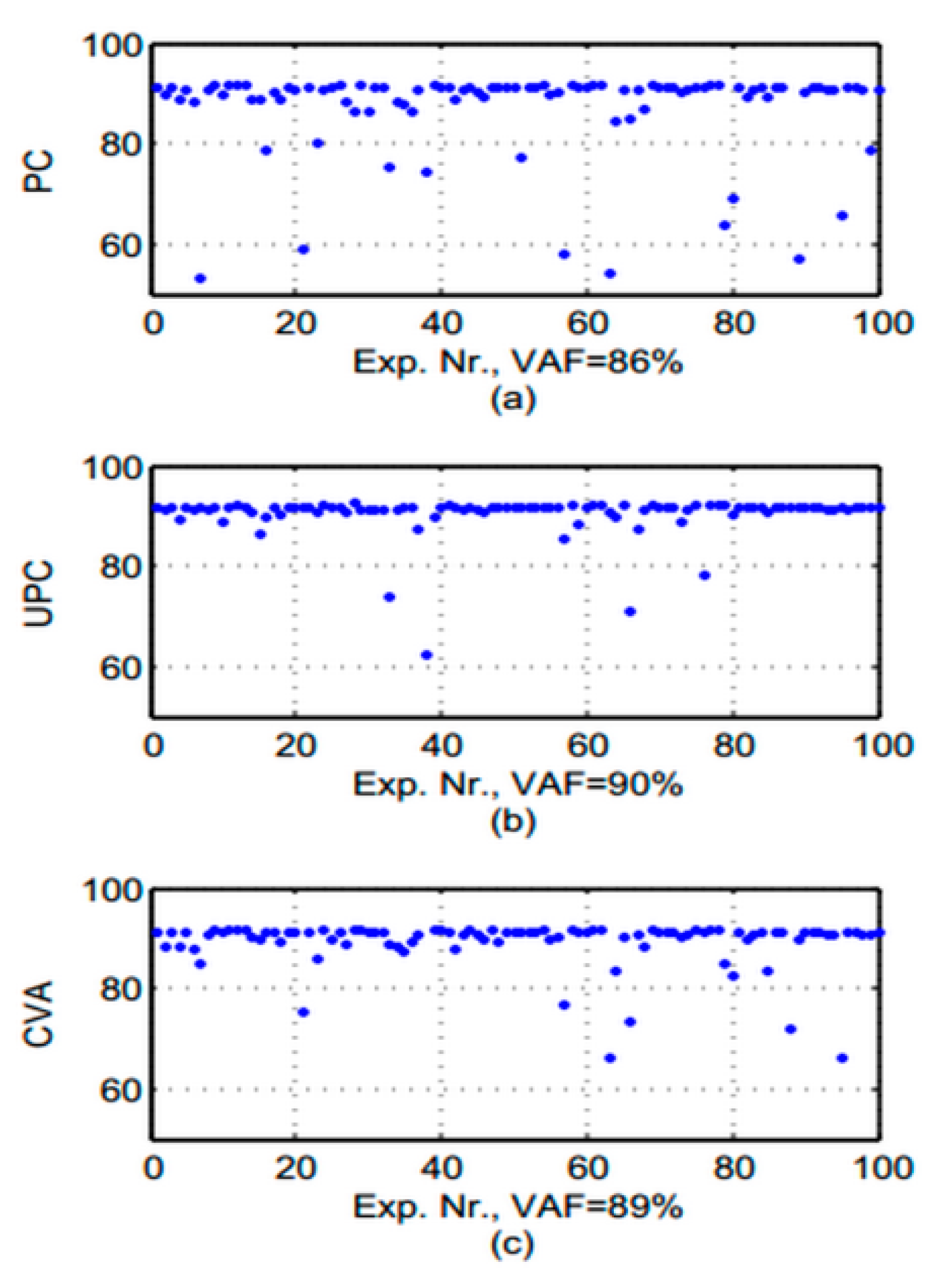
The extracted simulation response of the finite element model is used for the evaluation process. 100 different sets of noise patterns with the ratio of 30% were induced to the response signal in the fit analysis experiment. The VAF values of the noise-induced response signals are extracted and plotted in a
Figure 6.
The oscillation pattern of the weight matrices demonstrates that the UPC algorithm has the highest VAF value with less scattered data. It is an indicator of the outstanding prediction capability of the UPC method. The result of the PC and CVA method is only slightly worse. The lower ratios of the VAF values could be due to the short length of the response signal under influence of the damping effect.
3.2. Noise Robustness
Noise robustness of the CVA, UPC, and PC subspace algorithms are evaluated by plotting the extracted pole values. The obtained poles of a damped system are in the form of complex values. Though “complex poles” is a common term in analytical and experimental modal analysis, there is not any unified theory to normalize the obtained complex results [
44,
45]. Complex poles in a linear system contain real and imaginary parts. In an undamped system the real component of the complex modes are zero and the poles fall on imaginary axis. In the numerical model, the robustness of the subspace algorithms to noise uncertainty is evaluated by oscillation pattern of pole values in the noise-induced and reference states.
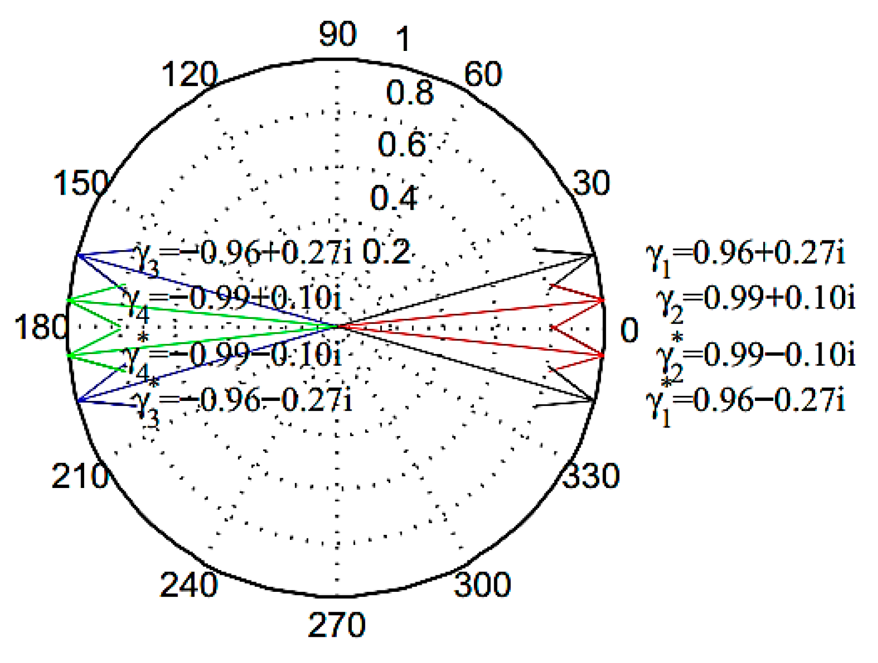
Figure 5 shows the first four orders of the system poles in the noise-free setting. The poles of the system are in the form of complex conjugates for each of the four orders. Hence,
and
are the first orders of the numerical model and
, and
are their conjugates. In a separate experiment incorporating noise ratios ranging from zero to 30% it was shown that he noise ratio of 5% provided a clear image transition of the patterns from the aggregated into the oscillated pattern. Hence the noise ratio of 5% was selected for plotting the pole analysis in the numerical model.
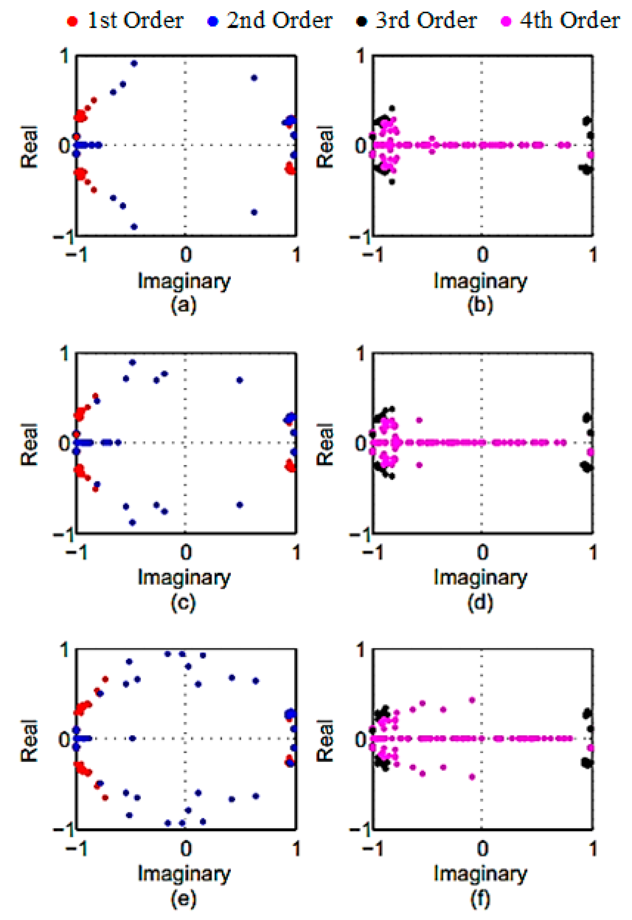
The identified results of the first four-orders using different SSI algorithms are plotted in complex plane as shown in
Figure 7 (The orders 1 and 2 and orders 3 and 4 are shown in separate figures). In order to provide the required data for this subsection, the response of the simulation model with the sampling frequency of 500 Hz was used for pole analysis. One hundred sets of different noise patterns were induced to the extracted response signal for evaluation of noise robustness.
Figure 8 shows the oscillation patterns of complex poles identified using the PC, UPC, and CVA. The conjugate pairs of the obtained pole values for the numerical model are symmetrically distributed about the real axes.
As it can be seen in the figure, aggregated complex pole values of the reference state can be traced from those of spattered noise-induced poles. The scatteration of pole values from the reference state is similar in UPC (
Figure 8a,b) and PC (
Figure 8c,d) algorithms whereas pole values obtained by UPC are slightly less affected by the noise variation). The CVA (
Figure 8e,f) algorithm has the highest scatteration among all subspace algorithms. The obtained result of the subspace algorithms show that the PC has the highest robustness against noise and for UPC algorithm is more affected by noise inclusion, while the CVA has the lowest robustness against noise in the conducted study.
3.3. Time Efficiency
Time efficiency is an important factor in implementation of an identification process. The elapsed computation time to identify a set of analysis process is used to compare the computation time of the CVA, PC, and UPC subspace algorithms. Time efficiency evaluation was carried out in a MSI Dual Core CPU desktop personal computer (3 GHz dual core CPU and 2 GB RAM) having Windows 7 as its operating system. Matlab software is used for all simulations, programing and analysis in this study. In order to simulate the response data obtained from the ambient excitation, random noise with ratio of 30% is added to the response signal of the numerical model. One hundred different noise-induced response signals are used in the evaluation process. The average elapsed time for identification of 100 sets of signals using CVA, PC and UPC algorithm was recorded as presented in
Table 1.
The mean values for identification of the system matrices using UPC, PC, and CVA are recorded 5.2, 10.8, and 11.3, respectively. The computation time for running CVA and PC algorithms is almost two fold higher than that of UPC for identification of the same set of input data. Higher performance of the UPC can be due to using unit weight matrix in the identification process.
4. Experimental Case Study
The benchmark vibration data from Alamosa Canyon Bridge in New Mexico,-USA is adopted for the experimental study. The experimental procedure for implementation and instrumentation of the vibration tests as well as the obtained response signals are made accessible through the Los Alamos National Laboratory’s (LANL) website [
46]. The benchmark dataset includes response signals extracted from the structure under artificial and natural excitation. These benchmark data have been used as experimental case study for many outstanding researches [
47,
48,
49].
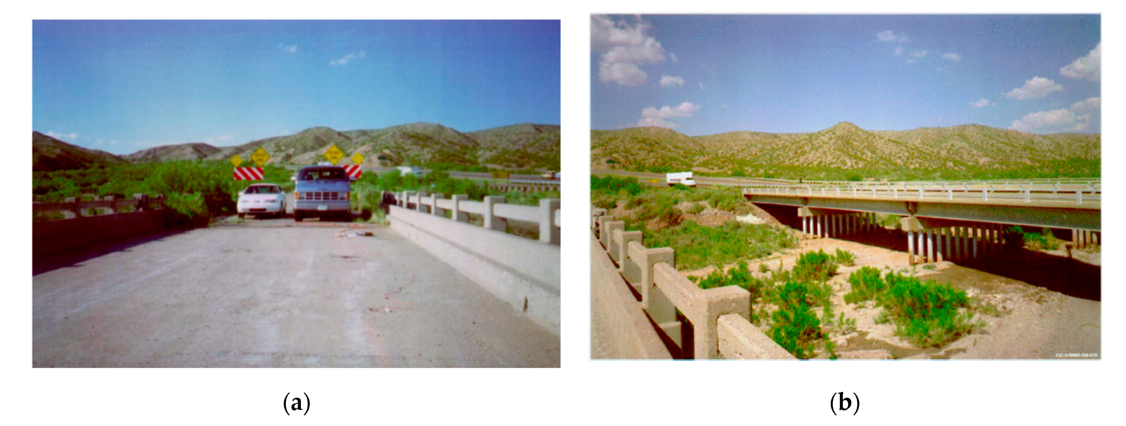
Figure 8 illustrates the ambient vibration test on the Alamosa Canyon Bridge. Dynamic load is applied to the structure by direct passing of a csar across the bridge deck and also by the traffic-induced ground vibration.
A direct vibration load was introduced by passing a typical car over the bridge. The car and the van containing the test instrumentation are shown in
Figure 9a. In order to introduce the ground-induced vibration into the structure a truck passing over the adjacent bridge was used as shown in
Figure 9b. The robustness of the subspace algorithms against the environmental and operational noise are evaluated using pole analysis. The acceleration response signals for the evaluation process are obtained from the accelerometers mounted on the bridge structure. A total of 30 accelerometers were installed within six rows in the widths of each deck and one accelerometer was mounted on the girder. The acceleration response time-histories are shrunk into groups of 1024 samples with the frequency of 50 Hz. The obtained signals are rearranged into 100 sets of five distinctive rows for the identification purpose [
50]. Unlike the numerical test in
Section 2 there is no access to the noise-free reference state of the real-world structures so, the optimum choice of the weight matrix is selected from the densest distribution of pole values in the complex plane plot.
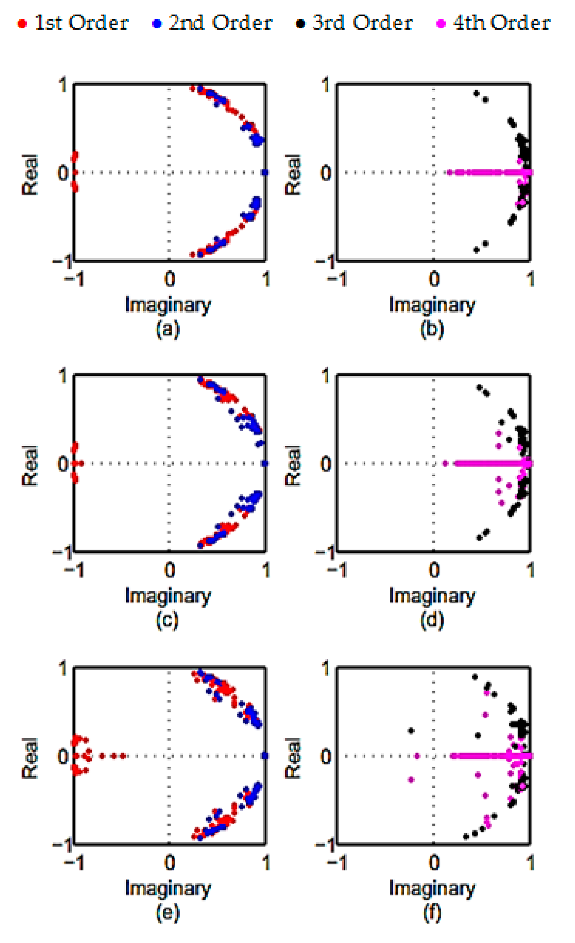
Figure 10 illustrates the results obtained for the comparison of the noise-robustness in subspace algorithms using pole analysis in the experimental model. Poles of the bridge structure lie inside a zero one plane. The scatteration of the conjugate poles is symmetric to real axes. The scatteration of poles in UPC algorithm (
Figure 10a,b) are more aggregated particularly in the 1st, 2nd, and 4th order. It means that the UPC algorithm is more robust to the noise variation compared to the other algorithms. Pole values obtained by PC algorithm (
Figure 10c,d) are more aggregated compared to CVA algorithm. The CVA (
Figure 10e,f) algorithm has the highest scatteration among all subspace algorithms.
The obtained result for the noise robustness of the subspace algorithms show that the PC is least affected by the noise inclusion.

 ,
, 


