Improved Homotopy Perturbation Method for Geometrically Nonlinear Analysis of Space Trusses


1
Department of Civil Engineering, Higher Education Complex of Bam, Bam 14477-76613, Iran
2
Department of Civil Engineering, Birjand University of Technology, Birjand 97175-569, Iran
3
Institute of Research and Development, Duy Tan University, Da Nang 550000, Vietnam
4
Department of Civil and Environmental Engineering, Virginia Tech, Blacksburg, VA 24061, USA
5
Department of Civil and Environmental Engineering, Incheon National University, Incheon 22012, Korea
6
Incheon Disaster Prevention Research Center, Incheon National University, Incheon 22012, Korea
*
Author to whom correspondence should be addressed.
Appl. Sci. 2020, 10(8), 2987; https://doi.org/10.3390/app10082987
Submission received: 1 March 2020
/
Revised: 17 April 2020
/
Accepted: 20 April 2020
/
Published: 24 April 2020
(This article belongs to the Special Issue Advances on Structural Engineering)
Abstract
:The objective of this study is to explore a noble application of the improved homotopy perturbation procedure bases in structural engineering by applying it to the geometrically nonlinear analysis of the space trusses. The improved perturbation algorithm is proposed to refine the classical methods in numerical computing techniques such as the Newton–Raphson method. A linear of sub-problems is generated by transferring the nonlinear problem with perturbation quantities and then approximated by summation of the solutions related to several sub-problems. In this study, a nonlinear load control procedure is generated and implemented for structures. Several numerical examples of known trusses are given to show the applicability of the proposed perturbation procedure without considering the passing limit points. The results reveal that perturbation modeling methodology for investigating the structural performance of various applications has high accuracy and low computational cost of convergence analysis, compared with the Newton–Raphson method.
1. Introduction
Truss systems are commonly implemented in several structural systems including space structures, high-span bridge systems and bracing the skeleton buildings. Recently, it is reported that the implementation of the linear analysis to investigate the structural applications is not sufficiently reliable without considering nonlinearities [1,2,3,4]. Instead, the development of engineering science and growth in computer processing power have made it possible to conduct an efficient nonlinear analysis. The linear theory is used for structures that are under service loads, but if there were slender elements in the structure or external loads exceeding the design loads (e.g., buckling load in the case of structural stability), ignorance of nonlinear behavior would cause considerable errors in a computational process due to large nonlinear deflections. Several studies in nonlinear analysis methods are presented [5,6,7,8,9], in which the stability of trusses under static and dynamic loads is investigated.
Along the same lines, Zhu et al. [10] studied geometric and material nonlinearity for space trusses. Large deformation of space trusses is investigated with a generalized displacement control method by Thai and Kim [11]. Greco and Ferreira [12] developed a new method for geometrically nonlinear analysis of the space trusses. Liu et al. [13] used perturbation algorithms for building membrane structure. There are many methods for nonlinear analysis such as iterative, incremental, and simple incremental–iterative methods. Along the same lines, Kao [14] compared the Newton–Raphson and incremental methods with geometrically nonlinear analysis, among which the Newton–Raphson method is used widely in nonlinear problems. Although this method is an efficient technique, a long computational cost is needed to achieve the convergence requirements [15].
Moreover, fast algorithms were presented to reduce the computational analysis of various structures [1,16,17,18,19,20,21,22]. An iterative perturbation method to solve a nonlinear system is proposed by Golbabi and Javidi [23]; however, the proposed method was not able to effectively reduce the convergence time despite reducing the number of iterations. In this paper, the presented method by Golbabi and Javidi [23] is improved to achieve an efficient nonlinear algorithm for further investigation of structures. The homotopy methodology is employed previously as a persice perturbation method for inelastic analysis of 2D frames [20]. The proposed procedures decrease both the iteration number and the cost of analysis. In this study, it is shown that the proposed methodology efficiently improves the inability of the Newton–Raphson algorithm in passing limit points due to load control limitations; hence, it improves the cost of analysis significantly.
2. Geometrically Nonlinear Analysis of Trusses
2.1. Geometrically Nonlinear Analysis of Trusses
The structural equilibrium equations are derived as [18]
where {f} is resultant internal forces based on the developed formed displacements coordinate, Pi represents the external forces, and n shows the number equilibrium equations. It is not possible to explicitly solve the load-deflection equations [13]. Hence, for a computational process, the equations’ incremental forms are considered as it is shown in Equations (2) and (3).
or
in which {Δu} indicates increments of displacements and [T] is the tangential stiffness for the considered system.
2.2. Tangent Stiffness Matrix for Members
The condition describing the forces at the end of members and end displacements is represented in Equation (4)
in which, {ΔP} is the load at each increment [T] is related to the member tangent stiffness given in Equation (5) and {Δu} is the increments of displacement [22], as illustrated in Figure 1.
in which, A is the cross-sectional area of the element; E represents the elastic modulus, the Q is the axial force in the truss member, L is the length of the member, {B} is transformation vector which summarizes the transformation from the global coordinate systems with local coordinates, and the geometric matrix [g] is given by Equation (6) [22].
where l, m, and n show the direction cosines of the member in the deformed shape and L’ describes the after-deformation length.
3. Nonlinear Analysis Algorithms
3.1. Newton–Raphson Method
The iterative Newton–Raphson method is commonly used for solving nonlinear structural systems. In this procedure, an approximate response is guessed for a structure described with nonlinear equations, and then an unknown corrector value is added to refine the initial response. Implementing approximation series (e.g., Taylor series), the nonlinear equations could be changed to a linear format equation, and by solving this linear system the corrector factor is achieved and the solution would be improved accordingly. This process is repeated until an acceptable approximation is obtained [25,26].
3.2. Improved Perturbation Method for the Nonlinear Problem
The perturbation method solution could be described as [27]
With boundary conditions shown in Equation (8). In Equation (7), u(x) denotes the approximation function of the solution.
where D is the differential operator and B indicates the boundary condition, and f(r(x)) is a general analytic function. If the Operator D is divided into two parts of linear LL and NL functions, the analytic function could be reestablished as shown in Equation (9).
Using the homotopy procedure over the constructed homotopy would result in
In which p is a small value between 0 and 1. u0(x) is the primary approximation response. Equation (10) could be described for specific p-values. Shown in Equations (11) and (12).
From the above-mentioned equations, it is concluded that varying p from zero to one is equivalent to varying H(U(x), p from LL(U(x)) − u0(x) to D(U(x)) − f(r(x)). By considering the perturbation technique, it could be assumed that the solution for Equations (11) and (12) are given as powers series of p.
From Equation (13) it is concluded that , which indicates the approximate solution. The equivalence convex homotopy is considered to illuminate NHPM solution procedure as it is indicated in Equation (14).
Equation (14) could be simplified and rewritten as shown in Equation (15)
Considering the S as the second derivative differential operator with respect to x (or d2/dx2), it is concluded that S−1 is the two-fold integration from 0 to x. Therefore, Equation (15) could be reestablished as shown in Equation (16).
It is noted that C is the constant incorporated in the integration; therefore, CS = 0. To apply the nonlinear perturbation method, the initial approximation is considered as shown in Equation (17).
where a0, a1, a2,.. are the unknown factors and F0(x), F1(x), F2(x), … are functions. In addition, if the factor p is considered as insignificant varying from the range 0 to 1, the solution for Equations (13) and (17) could be written as
If the coefficients of terms from the left-hand side and right-hand side of the Equation (18) are compared; therefore, Equation (19) could be obtained.
Therefore, the equations could be solved assuming that U1(x) = 0. Then from Equation (19), U2(x) = U3(x) =….= 0, Equation (20) could be obtained
3.3. Implementation of Perturbation Method in Structural Engineering
To use improved HPM, computational software is implemented for reducing the cost of analysis. The new approach uses Equations (13) to (20). Consider
where vector [13] denotes generalized coordinates established a base on the translations of nodes, {f} is resultant internal forces matrix and {F} is the external force matrix. Then
where J(u) is a Jacobian matrix that is required at each time increment and describes the local material behavior, [T] describes stiffness equations; therefore, Equation (22) can be rewritten as
First, an approximate solution is guessed similar to the Newton–Raphson method. An iterative algorithm based on previous formulations is developed for improving nonlinear analysis using the perturbation method. This algorithm is shown as follows:
Step 1: Input variables and parameters are set.
Step 2: The general assumptions related to the structural systems are considered (e.g., material properties, joint coordinates, boundary conditions, etc.).
Step 3: [T] is generated and assembled to summarize the stiffness equations to develop the system tangent stiffness matrix [τ].
Step 4: For the first iteration in (i + 1) loading step, the displacement is calculated.
Step 5: The new node coordinates are determined.
Step 6: The unbalanced forces in jth iteration is determined for (i + 1)th loading step {ΔQji+1 }.
Step 7: The {Duji+1} is calculated.
Step 8: Calculate the new geometry of the joints:
Step 9: Repeat steps 6–8 considering the convergence criterion is satisfied:
Step 10: Steps 6 through 8 are repeated to satisfy the convergence tolerance.
4. Results and Computational Examples
To compare the applicability of the proposed method with commonly used analysis methods in the nonlinear behavioral assessment of space trusses, four numerical examples are considered in a microcomputer environment. 32-bit Pentium 1.66 GHz processors (2 CPUs) is used for solving the numerical examples. For finding the nonlinear equation solutions, the proposed iterative method is implemented for which the iterative process is stopped as the convergence criteria are met. The tolerance of 10−4 is considered for evaluation purposes. In what follows, the four examples are discussed and analyzed with conventional and the proposed methods. In this paper, only geometric nonlinearity is considered in the numerical examples.
4.1. Example 1: 24-Member Space Truss
Figure 2 shows the first example of a three-dimensional space truss with two axes of a Cartesian coordinate system for which the z-axis represents the out-of-plane dimensions. As it is shown in Figure 2, a concentrated load is applied to the top of the dome-shaped space truss. The space truss consists of 24 members and 13 nodes in total, leading to 21 degrees of freedom. Based on the previously studied models, the modulus of elasticity E is 6895 kN/cm2, and area A is 6.452 cm2 and ΔP is considered to be 0.4448 kN.
Subsequently, the 3D truss is analyzed with the proposed PM method in this article and conventional Newton–Raphson. Figure 3 shows the displacement curve obtained separately based on each method and the computational cost for each method is summarized in Table 1. It is concluded that the PM method is able to precisely predict the behavior, while it reduces the computational cost by 10.9% and the number of iterations by 26.8% compared to classic Newton–Raphson.
4.2. Example 2: 42-Member Space Truss
The second space truss example is taken from Papadrakakis and Theoharis studies [9] which is schematically shown in Figure 4. The considered space truss consists of 42 members and 19 nodes. The pinned supports are considered as the boundary conditions. The identical cross-sectional properties are assumed for all the members and the material constitutive model has a module of elasticity of 211.67 kN/mm2. The section area is 16 mm2 and the concentrated force applied to the system is P = 0.135 N with ΔP = 0.03 N.
The load-displacement behavior of this model is shown in Figure 5. Table 2 shows the comparison of the classic Newton–Raphson with the perturbation method. It is concluded that the PM method is able to precisely evaluate the results, and reduce the computational cost and iteration number by 12.89% and 29.1%, respectively.
4.3. Example 3: 120-Member Space Truss
The third example shown in Figure 6 has 120 elements and 49 nodes. The boundary support condition is pinned to the ground. This example is based on the previous Saka and Ulker [29] studies on space trusses. It is noted that the axial stiffness (EA) is considered to be 44486.54 kN, and the concentrated load applied at the crown is equal to 1065 kN with a loading interval of 44.44 kN.
4.4. Example 4: 168-Member Space Truss
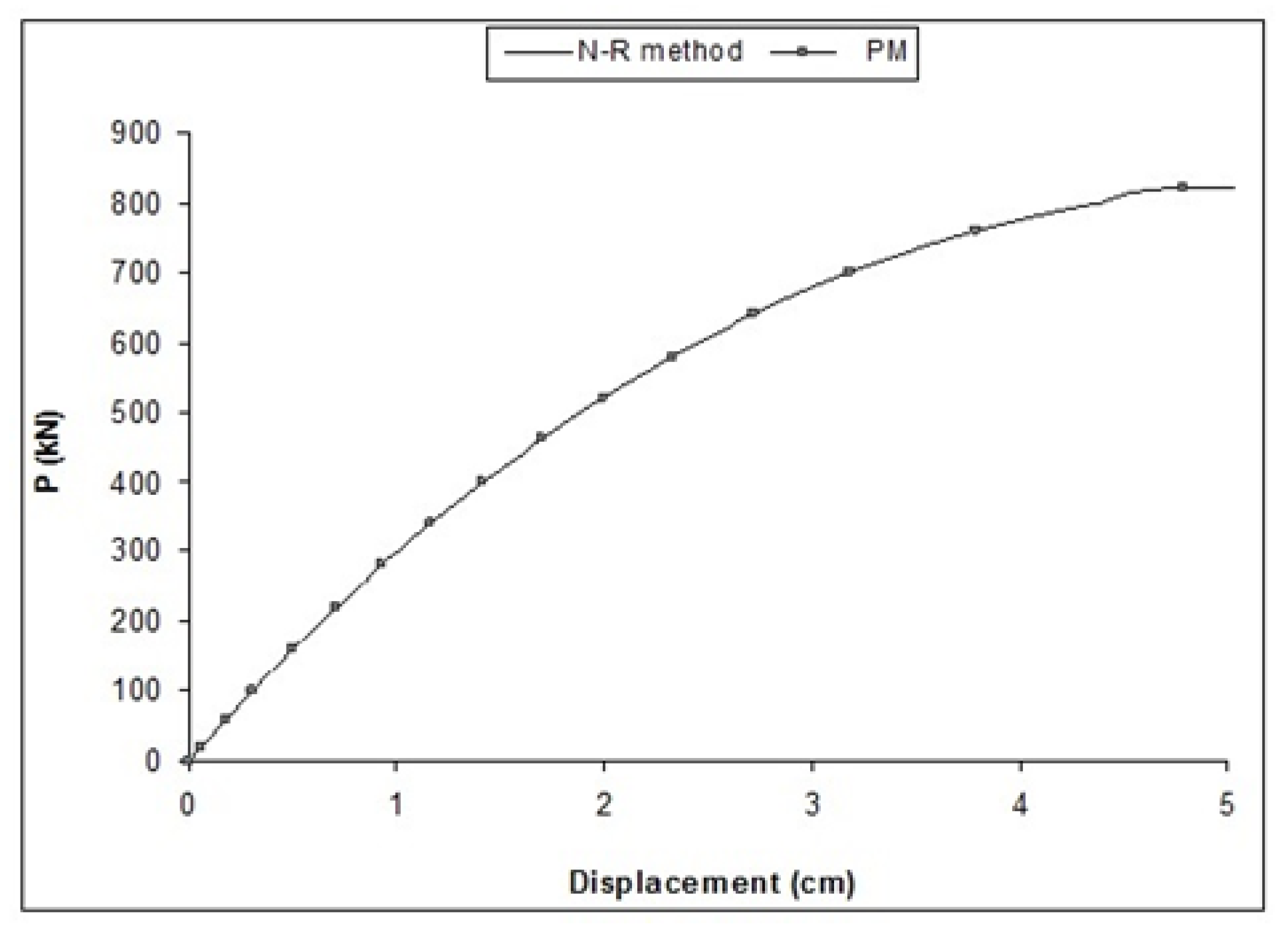
The fourth example is related to a dome truss extracted based on the previous studies [29] which is shown in Figure 8. The concentrated force of 820 KN is applied at the apex of 168 element truss with 73 nodes and 147 DOFs. It is noted that the out-of-plane motion is restrained for pinned supports for this structure. The cross-sectional area is 50.431 cm2 for all the members, and the material constitutive model has an elastic modulus of 2.04 × 10⁴ kN/cm2. The incremental load (ΔP) is 20 kN, which is applied at the apex of the structure.
5. Conclusions
A mathematical technique, referred to as the ‘perturbation method’ in this study, is proposed and applied for modeling space trusses with large displacements. The perturbation method approach is implemented for the nonlinear analysis of structures. The nonlinear system of equations is separated into portions of linear and nonlinear terms, and with iterative procedures, each set of equations is solved. This algorithm could be implemented for improving the nonlinear analysis according to the load control method based on the developed numerical process. It is shown that the perturbation method has the same precision compared to the classic Newton–Raphson method; however, it needs less computational work, iteration number, and computing time of analysis. It is shown that this method is a robust and efficient technique for nonlinear analysis of the large space trusses up to a limit, although the proposed procedure is incapable of tracing the equilibrium curve after the limit points.
Author Contributions
Conceptualization, H.D., I.M., A.F., and J.W.H.; Methodology, I.M., J.W.H.; Software, H.D., I.M.; Validation J.W.H. and A.F.; Formal Analysis A.F.; Investigation, A.F.; Resources, A.F.; Data Curation, J.W.H. and I.M.; Writing-Original Draft Preparation, J.W.H. and I.M.; Writing-Review & Editing, A.F., and J.W.H.; Visualization, H.D.; Supervision, I.M.; Project Administration, J.W.H.; Funding Acquisition, J.W.H. All authors have read and agreed to the published version of the manuscript.
Funding
This work was supported by a 2019 Incheon National University research grant. The authors gratefully acknowledge this supports.
Acknowledgments
This work was supported by a 2019 Incheon National University research grant. The authors gratefully acknowledge this supports.
Conflicts of Interest
The authors declare no conflict of interest.
References
- Saffari, H.; Baghlani, A.; Mirzai, N.M.; Mansouri, I. A new approach for convergence acceleration of iterative methods in structural analysis. Int. J. Comput. Methods 2013, 10, 1350022. [Google Scholar] [CrossRef]
- Rezaiee-Pajand, M.; Naserian, R. Using residual areas for geometrically nonlinear structural analysis. Ocean Eng. 2015, 105, 327–335. [Google Scholar] [CrossRef]
- Sangeetha, P.; Senthil, R. A study on ultimate behaviour of composite space truss. KSCE J. Civ. Eng. 2017, 21, 950–954. [Google Scholar] [CrossRef]
- Zhang, D.; Li, F.; Shao, F.; Fan, C. Evaluation of Equivalent Bending Stiffness by Simplified Theoretical Solution for an FRP–aluminum Deck–truss Structure. KSCE J. Civ. Eng. 2019, 23, 367–375. [Google Scholar] [CrossRef]
- Blandford, G.E. Large deformation analysis of inelastic space truss structures. J. Struct. Eng. 1996, 122, 407–415. [Google Scholar] [CrossRef]
- Hill, C.D.; Blandford, G.E.; Wang, S.T. Post-buckling analysis of steel space trusses. J. Struct. Eng. (United States) 1991, 117, 3829–3831. [Google Scholar] [CrossRef]
- Kassimali, A.; Bidhendi, E. Stability of trusses under dynamic loads. Comput. Struct. 1988, 29, 381–392. [Google Scholar] [CrossRef]
- Mansouri, I.; Farzampour, A. Buckling assessment of imperfect cylindrical shells under axial loading using a GEP technique. E-GFOS 2018, 9, 89–100. [Google Scholar] [CrossRef]
- Papadrakakis, M.; Theoharis, A.P. Tracing post-limit-point paths with incomplete or without factorization of the stiffness matrix. Comput. Methods Appl. Mech. Eng. 1991, 88, 165–187. [Google Scholar] [CrossRef]
- Zhu, K.; Al-Bermani, F.G.A.; Kitipornchai, S. Nonlinear dynamic analysis of lattice structures. Comput. Struct. 1994, 52, 9–15. [Google Scholar] [CrossRef]
- Thai, H.T.; Kim, S.E. Large deflection inelastic analysis of space trusses using generalized displacement control method. J. Constr. Steel Res. 2009, 65, 1987–1994. [Google Scholar] [CrossRef]
- Greco, M.; Ferreira, I.P. Logarithmic strain measure applied to the nonlinear positional formulation for space truss analysis. Finite Elem. Anal. Des. 2009, 45, 632–639. [Google Scholar] [CrossRef]
- Liu, C.J.; Zheng, Z.L.; Yang, X.Y.; Guo, J.J. Geometric Nonlinear Vibration Analysis for Pretensioned Rectangular Orthotropic Membrane. Int. Appl. Mech. 2018, 54, 104–119. [Google Scholar] [CrossRef]
- Kao, R. A comparison of Newton-Raphson methods and incremental procedures for geometrically nonlinear analysis. Comput. Struct. 1974, 4, 1091–1097. [Google Scholar] [CrossRef]
- Batoz, J.-L.; Dhatt, G. Incremental displacement algorithms for nonlinear problems. Int. J. Numer. Methods Eng. 1979, 14, 1262–1267. [Google Scholar] [CrossRef]
- Lee, H.-W.; Cho, J.-R. Geometrically Non-linear Analysis of Elastic Structures by Petrov-Galerkin Natural Element Method. KSCE J. Civ. Eng. 2019, 23, 1756–1765. [Google Scholar] [CrossRef]
- Mansouri, I.; Saffari, H. An efficient nonlinear analysis of 2D frames using a Newton-like technique. Arch. Civ. Mech. Eng. 2012, 12, 485–492. [Google Scholar] [CrossRef]
- Mansouri, I.; Saffari, H. Geometrical and material nonlinear analysis of structures under static and dynamic loading based on quadratic path. Sci. Iran. 2013, 20, 1595–1604. [Google Scholar]
- Mansouri, I.; Saffari, H. A fast hybrid algorithm for nonlinear analysis of structures. Asian J. Civ. Eng. 2014, 15, 213–230. [Google Scholar]
- Saffari, H.; Mansouri, I.; Bagheripour, M.H.; Dehghani, H. Elasto-plastic analysis of steel plane frames using Homotopy Perturbation Method. J. Constr. Steel Res. 2012, 70, 350–357. [Google Scholar] [CrossRef]
- Saffari, H.; Mirzai, N.M.; Mansouri, I. An accelerated incremental algorithm to trace the nonlinear equilibrium path of structures. Lat. Am. J. Solids Struct. 2012, 9, 425–442. [Google Scholar] [CrossRef] [Green Version]
- Saffari, H.; Mirzai, N.M.; Mansouri, I.; Bagheripour, M.H. Efficient numerical method in second-order inelastic analysis of space trusses. J. Comput. Civil. Eng. 2013, 27, 129–138. [Google Scholar] [CrossRef]
- Golbabai, A.; Javidi, M. Newton-like iterative methods for solving system of non-linear equations. Appl. Math. Comput. 2007, 192, 546–551. [Google Scholar] [CrossRef]
- Lebofsky, S. Numerically Generated Tangent Stiffness Matrices for Geometrically Non-Linear Structures. Master’s Thesis, University of Washington, Washington, DC, USA, 2013. [Google Scholar]
- Crisfield, M.A. Nonlinear Finite Element Analysis of Solid and Structure; John Wiley: Hoboken, NJ, USA, 2006. [Google Scholar]
- Bhatti, M. Advanced Topics in Finite Element Analysis of Structure; John Wiley: Hoboken, NJ, USA, 2006. [Google Scholar]
- Vahidi, A.R.; Babolian, E.; Azimzadeh, Z. An Improvement to the Homotopy Perturbation Method for Solving Nonlinear Duffing’s Equations. Bull. Malays. Math. Sci. Soc. 2018, 41, 1105–1117. [Google Scholar] [CrossRef]
- Saffari, H.; Mansouri, I. Non-linear analysis of structures using two-point method. Int. J. Nonlin. Mech. 2011, 46, 834–840. [Google Scholar] [CrossRef]
- Saka, M.P.; Ulker, M. Optimum design of geometrically nonlinear space trusses. Comput. Struct. 1992, 42, 289–299. [Google Scholar] [CrossRef]
Figure 1.
Incremental–iterative solution method [24].
Figure 1.
Incremental–iterative solution method [24].

Figure 2.
Space truss with 24–members, all dimensions are in mm [28].
Figure 2.
Space truss with 24–members, all dimensions are in mm [28].
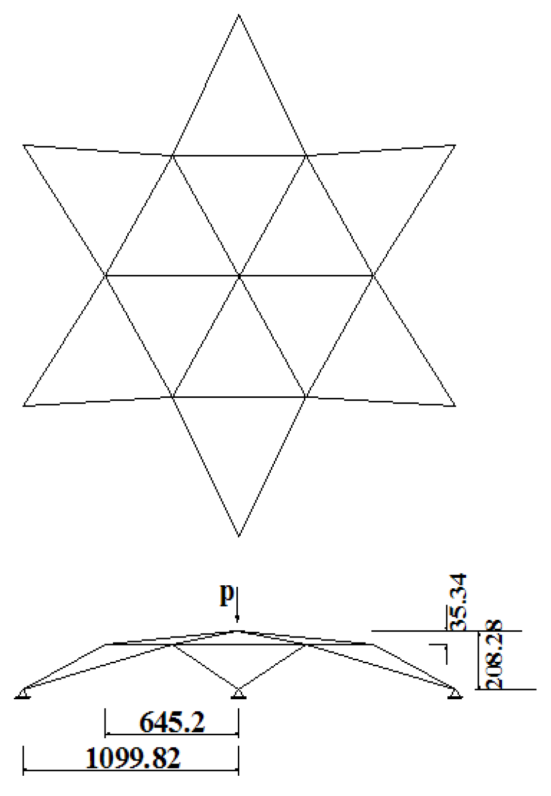
Figure 3.
Space truss with 24–members, all dimensions are in mm.
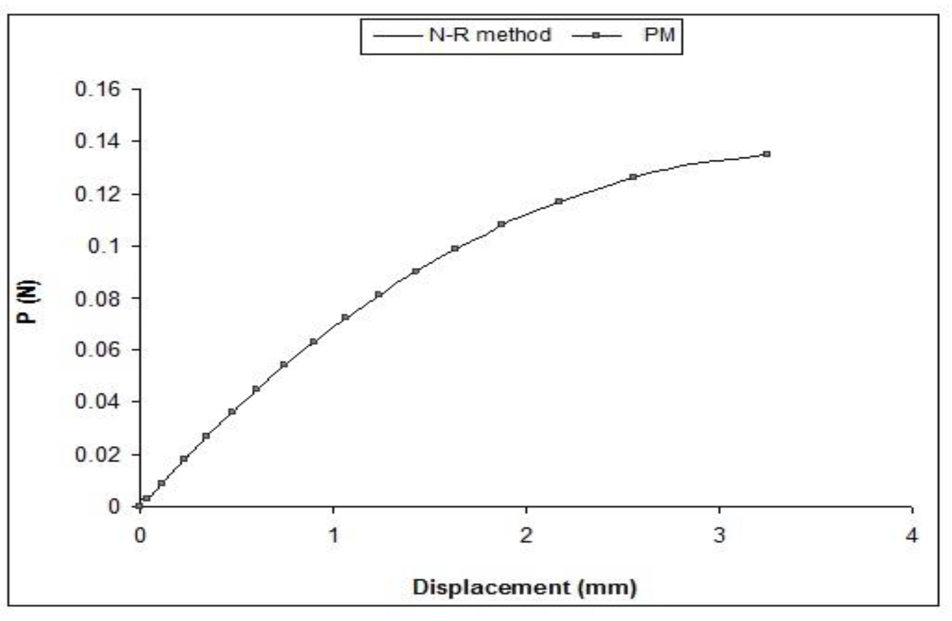
Figure 4.
Space truss with 42–members, all dimensions are in mm [28].
Figure 4.
Space truss with 42–members, all dimensions are in mm [28].
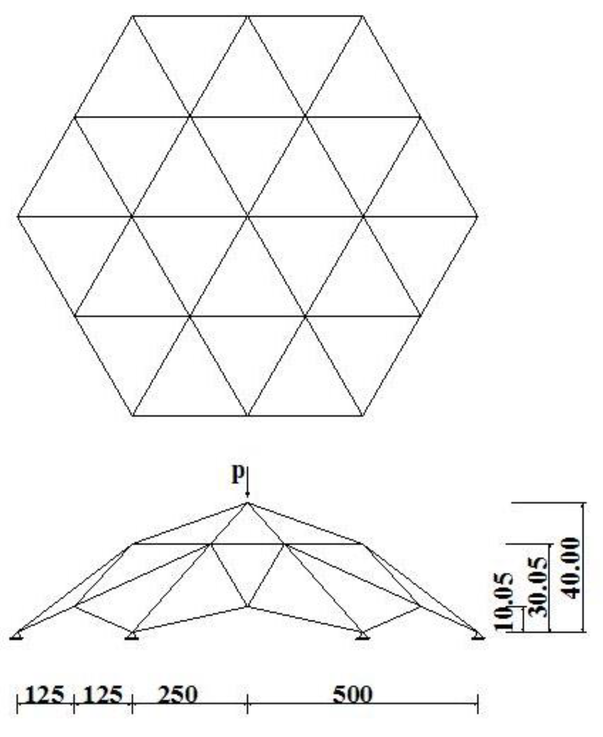
Figure 5.
Space truss with 42–members, all dimensions are in mm.
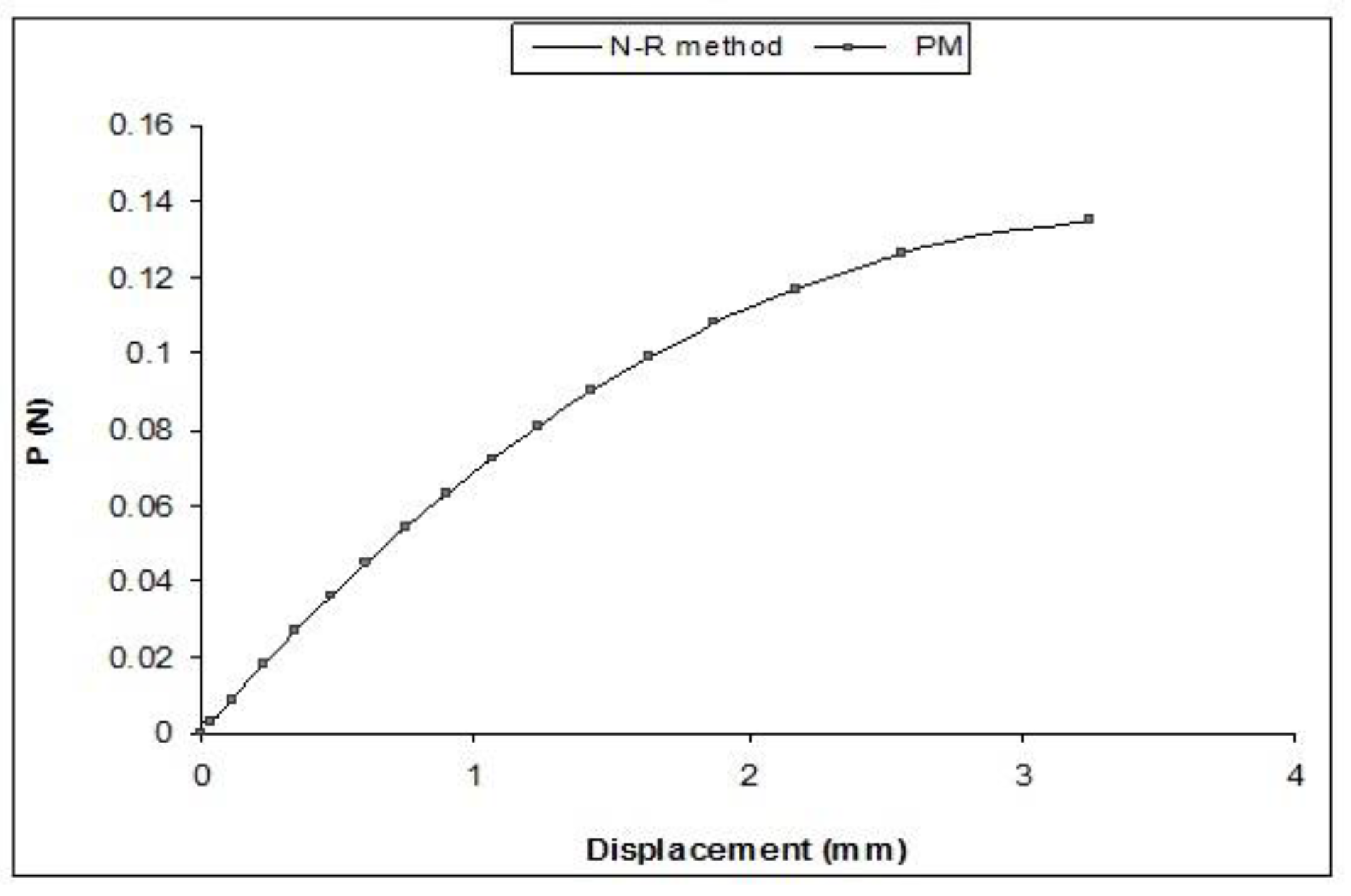
Figure 6.
Space truss with 120–members, all dimensions are in mm [28].
Figure 6.
Space truss with 120–members, all dimensions are in mm [28].
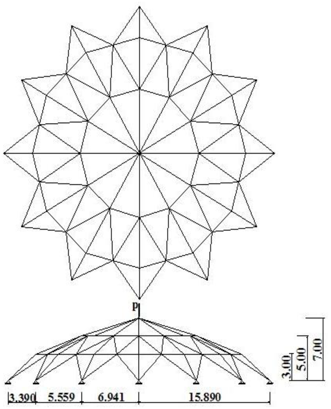
Figure 7.
Space truss with 120–members, all dimensions are in mm.
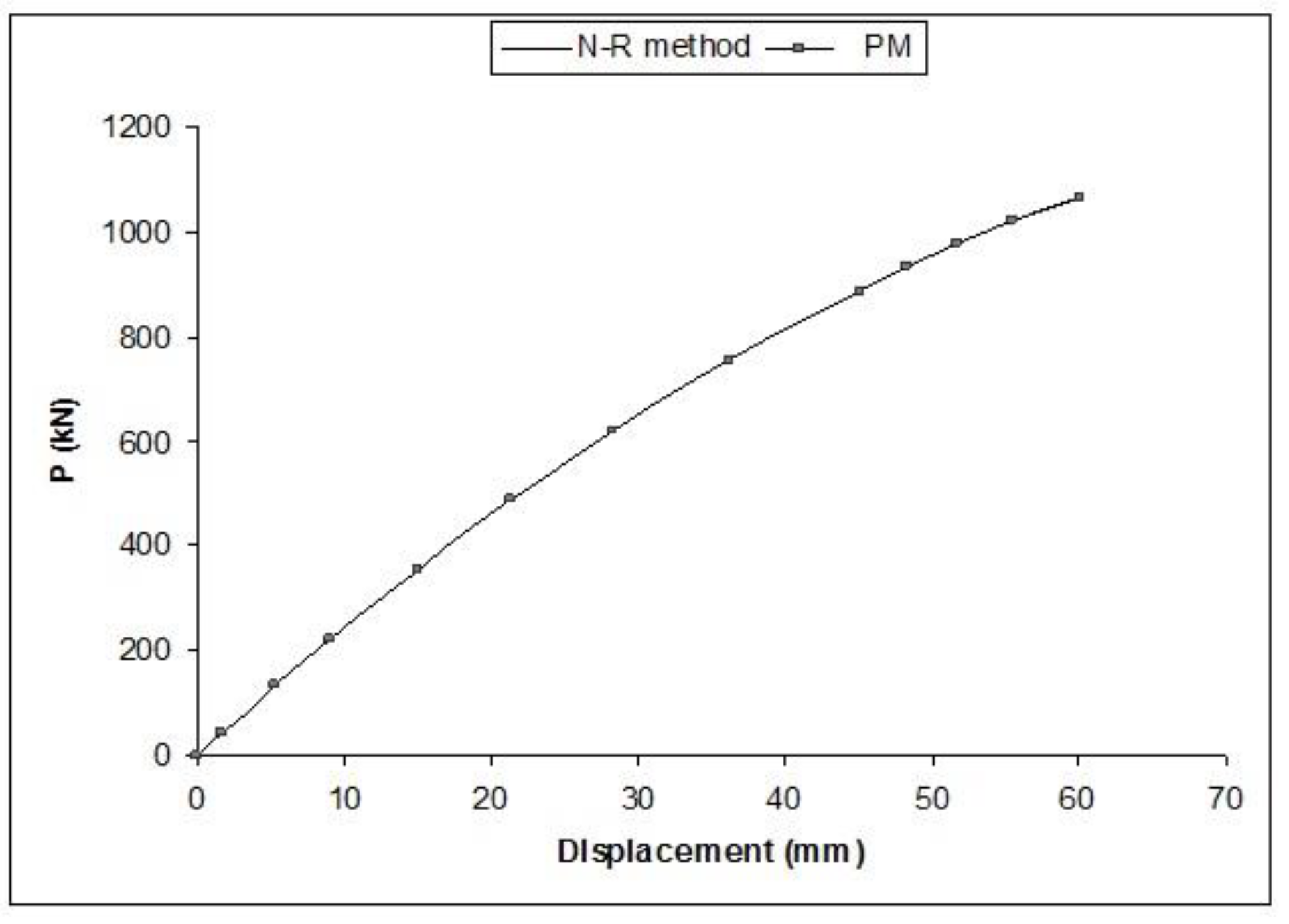
Figure 8.
Space truss with 168–members, all dimensions are in mm [28].
Figure 8.
Space truss with 168–members, all dimensions are in mm [28].
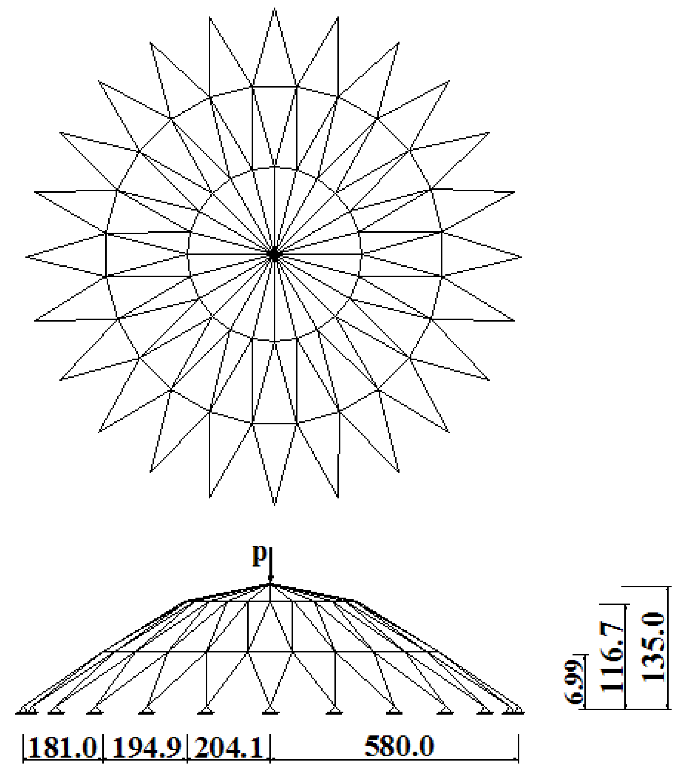
Figure 9.
Space truss with 168–members, all dimensions are in mm.

Table 1.
Comparison of the computational cost and iteration number
| Decrease Percentage | Present Method | Newton Method | |||
|---|---|---|---|---|---|
| Iteration no. | Time (s) | Iteration No. | Time (s) | Iteration No. | Time (s) |
| 27 | 10.93 | 79 | 0.145 | 108 | 0.1628 |
Table 2.
Comparison of computational cost and iteration number
| Decrease Percentage | Present Method | Newton Method | |||
|---|---|---|---|---|---|
| Iteration no. | Time (s) | Iteration No. | Time (s) | Iteration No. | Time (s) |
| 29 | 12.89 | 107 | 0.3107 | 151 | 0.3567 |
Table 3.
Comparison of the computational cost and iteration number
| Decrease Percentage | Present Method | Newton Method | |||
|---|---|---|---|---|---|
| Iteration No. | Time (s) | Iteration No. | Time (s) | Iteration No. | Time (s) |
| 31 | 10.43 | 51 | 0.4894 | 74 | 0.5464 |
Table 4.
Comparison of computational cost and iteration number
| Decrease Percentage | Present Method | Newton Method | |||
|---|---|---|---|---|---|
| Iteration No. | Time (s) | Iteration No. | Time (s) | Iteration No. | Time (s) |
| 29 | 8.79 | 88 | 1.224 | 124 | 1.342 |
© 2020 by the authors. Licensee MDPI, Basel, Switzerland. This article is an open access article distributed under the terms and conditions of the Creative Commons Attribution (CC BY) license (http://creativecommons.org/licenses/by/4.0/).
Share and Cite
MDPI and ACS Style
Dehghani, H.; Mansouri, I.; Farzampour, A.; Hu, J.W. Improved Homotopy Perturbation Method for Geometrically Nonlinear Analysis of Space Trusses. Appl. Sci. 2020, 10, 2987. https://doi.org/10.3390/app10082987
AMA Style
Dehghani H, Mansouri I, Farzampour A, Hu JW. Improved Homotopy Perturbation Method for Geometrically Nonlinear Analysis of Space Trusses. Applied Sciences. 2020; 10(8):2987. https://doi.org/10.3390/app10082987
Chicago/Turabian StyleDehghani, Hamzeh, Iman Mansouri, Alireza Farzampour, and Jong Wan Hu. 2020. "Improved Homotopy Perturbation Method for Geometrically Nonlinear Analysis of Space Trusses" Applied Sciences 10, no. 8: 2987. https://doi.org/10.3390/app10082987
Note that from the first issue of 2016, this journal uses article numbers instead of page numbers. See further details here.