Impacts of Weather on Short-Term Metro Passenger Flow Forecasting Using a Deep LSTM Neural Network

Abstract

Metro systems play a key role in meeting urban transport demands in large cities. The close relationship between historical weather conditions and the corresponding passenger flow has been widely analyzed by researchers. However, few studies have explored the issue of how to use historical weather data to make passenger flow forecasting more accurate. To this end, an hourly metro passenger flow forecasting model using a deep long short-term memory neural network (LSTM_NN) was developed. The optimized traditional input variables, including the different temporal data and historical passenger flow data, were combined with weather variables for data modeling. A comprehensive analysis of the weather impacts on short-term metro passenger flow forecasting is discussed in this paper. The experimental results confirm that weather variables have a significant effect on passenger flow forecasting. It is interesting to find out that the previous variables of one-hour temperature and wind speed are the two most important weather variables to obtain more accurate forecasting results on rainy days at Taipei Main Station, which is a primary interchange station in Taipei. Compared to the four widely used algorithms, the deep LSTM_NN is an extremely powerful method, which has the capability of making more accurate forecasts when suitable weather variables are included.

1. Introduction

As one of the most important issues in an urban metro system is part of smart cities [1], passenger flow analysis and forecast for public transport have been widely studied over the last two decades. Metro systems play an important role in meeting urban transport demand. Because of their high speed, efficiency, volume, and punctuality, urban metros are the first choice for many daily commutes [2]. More accurate short-term passenger flow forecasting for metro systems is important in solving a series of problems in the process of urban development, such as mitigating the adverse effects of traffic congestion, reducing vehicle pollution, better planning of public transit networks, and better land use planning along metro lines.

Following an overview of the previous studies, we can conclude that the issue of short-term passenger flow forecasting is an ongoing process, primarily studied from two perspectives, namely data modeling and methodology modeling. In the field of data modeling, accurately forecasting passenger flow is fairly challenging because many factors affect the target station’s passenger flow [3]. The most widely used input variables are historical passenger flow data and their corresponding spatiotemporal data. Although experimental results show that weather data [4,5] were able to represent the passenger flow, only limited research efforts have been directed to the issue of passenger flow forecasting with the weather factor due to the difficulties in data acquisition and data fusion among weather data, spatiotemporal data, and historical passenger flow data [6]. More researchers have preferred to analyze the relationship between historical weather conditions and the corresponding historical passenger flow, especially focusing on the negative impacts of inclement weather on passenger demand [7,8]. The problems of the impacts of weather on passenger flow forecasting in the available literature are described as follows.

First, due to the scarcity of dynamic passenger flow data caused by weather factors, the addition of one weather variable, or especially multiple weather variables, would not improve the forecasting accuracy, which would even decrease [9]. Thus, some researchers have only added one weather variable for passenger flow forecasting. For example, Ke et al. [9] used random forest (RF) to rank the importance of all the input variables, including the five weather variables, namely temperature, humidity, weather state, wind speed, and visibility, while only temperature was quantified as the dominating weather factor for developing a short-term forecasting of passenger demand under an on-demand ride service platform in Hangzhou. Tang et al. [10] evaluated the rain effect on short-term passenger flow forecasting for the Shenzhen metro. Chen et al. [11] proposed a short-term prediction of passenger flow on bus routes in Changsha by considering rainfall intensity. Liu et al. [12] proposed a short-term passenger flow forecasting model of four bus lines under rainy conditions. Furthermore, to extensively explore the impacts of multiple weather variables on passenger flow forecasting, more than one weather variable was used together to build the models. For example, Li et al. [13] applied wind power, average temperature, dew point temperature, air quality index, humidity, rainfall, and cloud cover as the exogenous input variables to propose a forecasting model of station passenger flows for Shanghai rail transit. However, it did not explicitly indicate if the forecasting performance had improved or not using the seven weather variables. Wan et al. [14] selected weather conditions (i.e., sunny, cloudy, etc.), wind direction and speed, temperature, humidity, and air pressure for the prediction of passenger demand for different air routes. However, these weather variables, combined with day of the week and holiday, are all defined as exogenous input variables. Although the experiment verified that the proposed model with such exogenous input variables was better than that without the exogenous input variable module, it did not powerfully verify whether the addition of weather variables would be helpful for improving the forecasting performance.

Second, most studies have aggregated daily and monthly passenger flows with weather data to explain the daily and seasonal ridership variation. For example, Stover et al. [15] examined the effects of temperature, rainfall, wind speed, and snow on daily bus ridership forecasting for Pierce County, Washington, during 2006–2008. The results showed that each weather variable had a significant effect on bus ridership for at least one season. Bocker et al. [16] provided a systematic and comprehensive overview to evaluate the impact of daily weather on individual daily travel activities. The results showed that rain, snow, wind, and temperature could influence the travel behavior, departure time, travel time, and routes. Liu et al. [17] investigated the seasonal and regional impacts of weather conditions on individual travel mode choice in Sweden by using the weather and travel data for 13 years with the multinomial logit method. The findings showed the existence of seasonal and regional variances, indicating that the weather contributed to individual travel mode choice. The literature [15,16,17] reviewed above indicates that such day-level or season-level studies do not clearly distinguish daily travel pattern changes, especially during the morning and evening peak hours. The study of weather impacts on hourly passenger flow forecasting may be more meaningful than daily, monthly, or seasonal passenger flows, which can reduce the negative impacts of weather on daily commutes.

In the field of methodology modeling, many successful and high-performance passenger flow forecasting models have been proposed by using different methodologies. The authors in [18] summarized them into two categories, namely parametric methods and non-parametric methods. In a data-rich environment, deep neural network-based models, especially sequence models such as recurrent neural network (RNN) [19], long short-term memory neural network (LSTM_NN) [20], and gate recurrent unit neural network (GRU_NN) [21], have been comprehensively applied to traffic flow forecasting. An RNN-based microscopic car-following model was developed to capture and accurately predict traffic oscillation in Emeryville, California [22]. The results indicated that RNN had a stronger performance in predicting the trajectories of a group of subsequent vehicles given the trajectory of the first vehicle and initial/boundary conditions for the following vehicles. A novel traffic volume forecasting model based on an LSTM_NN was proposed in [23]. The experimental results showed that the proposed LSTM_NN was more robust for traffic volume forecasting than other state-of-the-art methodologies. A deep GRU-based car-following model was proposed to better capture and describe the complicated human behaviors [24]. The data were retrieved from the southbound direction of U.S. Highway 101 in Los Angeles, California.

In summary, motivated by the close relationship between passenger flow and weather conditions, and along with the high-performance of an LSTM_NN in traffic flow forecasting, we applied a deep LSTM_NN to develop a metro passenger flow forecasting model by fusing historical hourly passenger flow data and the corresponding temporal and weather data in a station-level study. The main contributions of this paper are as follows.

(1) An hourly passenger flow forecasting model considering weather conditions was developed by using a deep LSTM_NN. The single weather variable of temperature, wind speed, relative humidity, and rainfall, as well as their various combinations, were separately assembled with the temporal data and historical passenger flow data, to build a series of station-level forecasting models to comprehensively analyze the impacts of different weather conditions on hourly metro passenger flow forecasting. Researchers have widely applied a deep LSTM_NN in building a passenger flow forecasting model, but rarely have they used it to build a forecasting model to comprehensively analyze the impacts of different weather conditions on passenger flow forecasting in such detail.

(2) The majority of weather data present general variations, which do not have much impact on passengers’ daily commuting, even in the case of heavy rain. This indicates that adding the weather data as inputs to build a forecasting model may not be helpful in improving the forecasting results, because the weather data are likely noisy data in comparison with the temporal data and historical passenger flow data. Furthermore, the study of weather impacts on hourly passenger flow forecasting may be more meaningful than daily, monthly, or seasonal passenger flows. In these cases, how to select the suitable weather data to develop a short-term passenger forecasting model with higher performance is challenging. The experimental results powerfully verified that adding the previous variables of one-hour temperature and wind speed could indeed improve the results in comparison with the model using no weather data for hourly metro passenger flow forecasting at Taipei Main Station on rainy days.

The remainder of this paper is organized as follows. Section 2 describes the station-level passenger demand in the Taipei Mass Rapid Transit (MRT). The input variables used and the impacts of weather on hourly passenger flow are also analyzed in this section. Section 3 introduces the architecture of a cell in LSTM and the dataflow of the deep LSTM_NN in this paper. A case study of Taipei Main Station is presented in Section 4 in detail, and the experimental results are analyzed comprehensively against RF and the other three deep neural networks. Section 5 concludes the paper and suggests directions for future study.

2. Input Variables

The hourly inbound and outbound flows in the Taipei MRT have been available from the Taipei city government’s open dataset since 1 November 2015 [25]. Figure 1 shows that Taipei Main Station has the highest average daily passenger flow. Its inbound and outbound flow is twice the second highest total of the top ten stations in Taipei. Therefore, Taipei Main Station was selected as a case study in the experimental section.

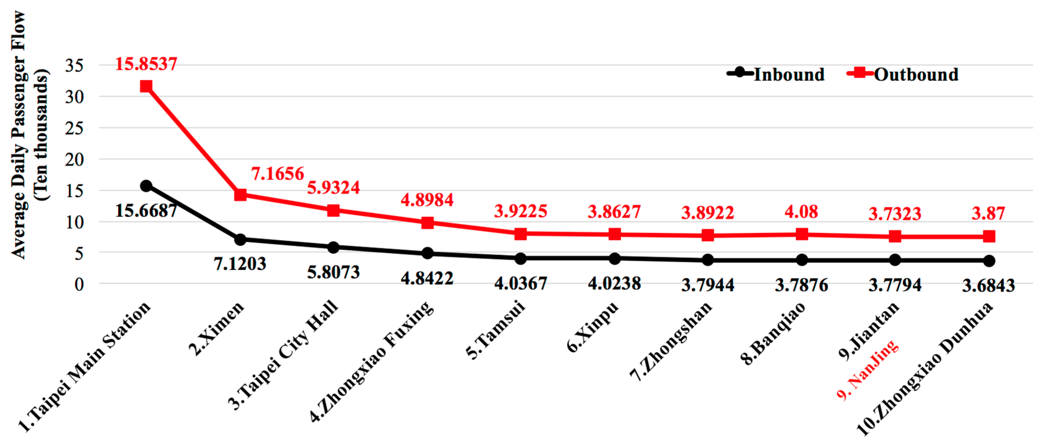
2.1. Station-level Data Description

As shown in

Table 1. Detailed information of the training data and testing data for Taipei Main Station.

Item		Training Dataset	Testing Dataset
Duration		1 November 2015–31 October 2016	1 November 2016–31 March 2017
Outlier		8 July 2016; 27 September 2016; 28 September 2016	None
Number of days		363	151
Number of national holidays		31	13
Operating hours	Inbound	0:00, 5:00–23:00
	Outbound	0:00, 6:00–23:00
Special examples to be added	Inbound	1:00–4:00 on 1 January 2016	1:00–4:00 on 1 January 2017
	Outbound	1:00–5:00 on 1 January 2016	1:00–5:00 on 1 January 2017
Special examples to be deleted		0:00 on 1 November 2015
Time interval		One hour
Total examples	Inbound	7263	3024
	Outbound	6901	2874
	National holiday	1218	516
	Non-national holiday	12,946	5382
Total Examples		14,164	5898

, we used the data of 363 days from 1 November 2015, to 31 October 2016 for training, and the remaining 151 days from Nov. 1, 2016, to Mar. 31, 2017 for testing. The ratio of training data and testing data was nearly 7:3. A detailed description of the data used for Taipei Main Station is given in Table 1.

2.2. Endogenous Input Variables

The traditional input variables, namely passenger flow direction ($v_{Dir}$), date (month ($v_M$), day ($v_D$)), week ($v_W$), hour ($v_H$), national holiday ($v_{NH}$), previous average hourly passenger flow ($v_{\overline{Pre\_PF}}$), previous 1-hour, 2-hour, 3-hour passenger flow ($v_{PF\_Pre\_1},v_{PF\_Pre\_2},v_{PF\_Pre\_3}$), and previous 2-hour passenger flow trend ($v_{PFTr\_Pre\_2}$), are defined as the endogenous input variables in this paper. The results in [26] show that the above endogenous input variables are the optimized combination for developing a high-performance model for passenger flow forecasting. Thus, all of them were used in the experiment.

2.3. Exogenous Input Variables

Because of the potential relationship between weather conditions and urban transit ridership, weather variables were defined as the exogenous input variables in this paper. The weather data were provided by the Taiwan Environmental Protection Administration (Taiwan EPA) [27]. An extensive review of the previous literature [4,5,6,7,8,9,10,11,12,13,14,15,16,17] showed that temperature ($v_{Temp}$), rainfall ($v_{Rain}$), relative humidity ($v_{Hum}$), wind speed ($v_{Wind}$), and snow ($v_{Snow}$) were the most commonly used weather variables. Because Taipei almost never sees snow, $v_{Temp}$, $v_{Rain}$, $v_{Hum}$, and $v_{Wind}$ were selected as the four weather variables in the study. The weather data were available from the Zhongshan meteorological monitoring station, which is the nearest observation station to Taipei Main Station. The weather data were hourly, which has the same time interval as the endogenous input variables described in Section 2.2.

2.4. Analysis of Impacts of Weather Conditions on Hourly Passenger Flow

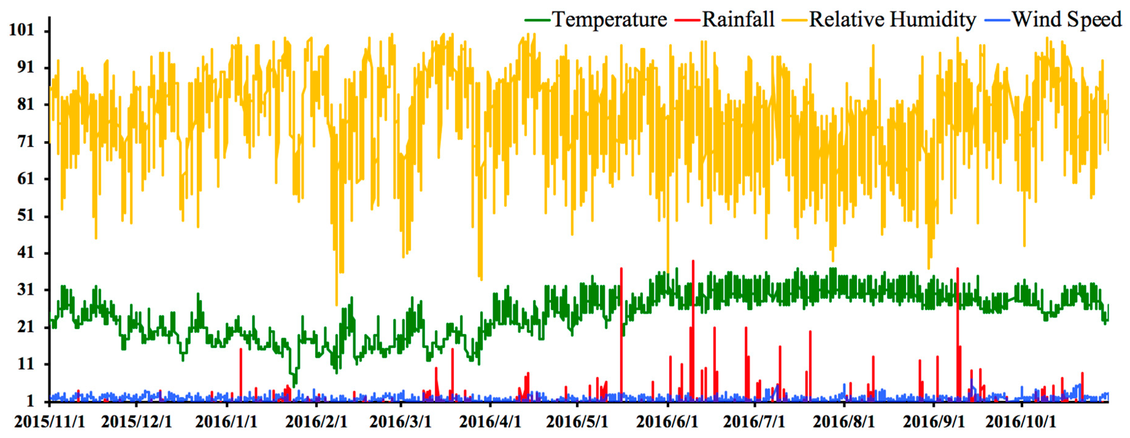
2.4.1. Overview of Annual Weather Conditions in Taipei

Taipei is a typical city with a subtropical monsoon climate. Figure 2 shows the historical annual weather information from 1 November 2015 to 31 October 2016 around Taipei Main Station. Rainfall was copious throughout the year, especially June through September. However, heavy rainfall was uncommon. The temperatures were usually pleasantly warm with a high relative humidity. The winter months from December to February were colder with a relatively low temperature, less than 20 °C.

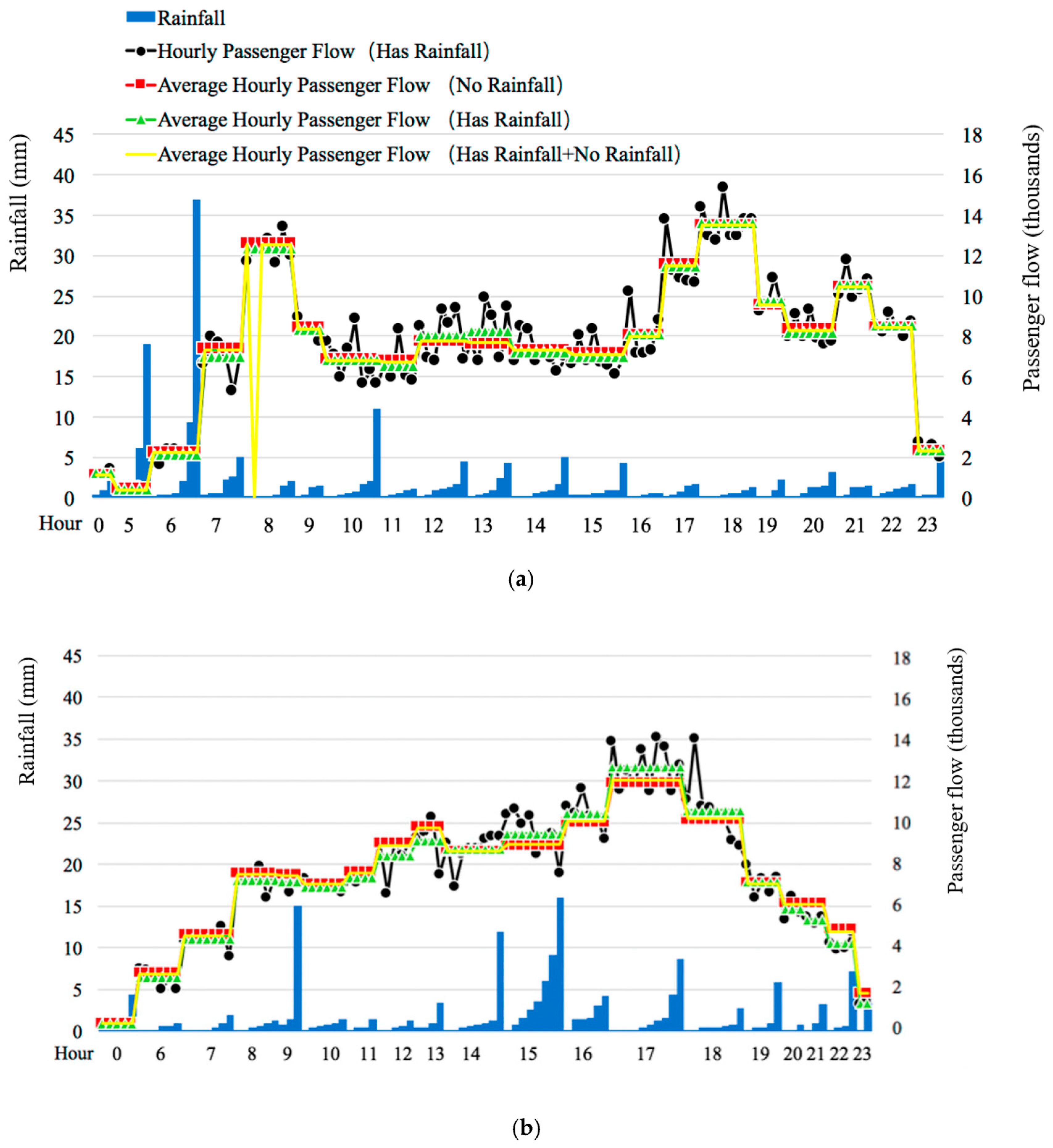
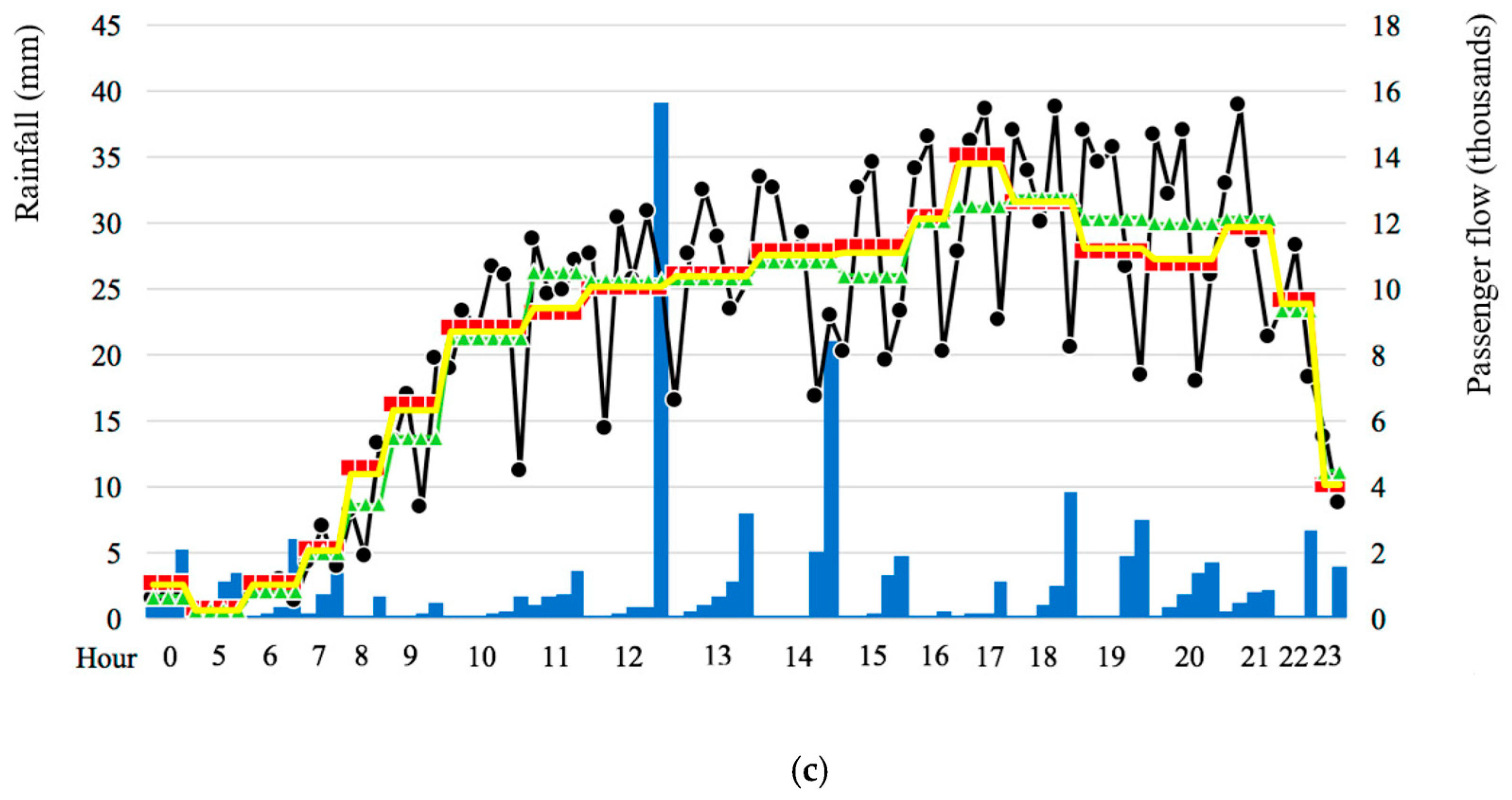
2.4.2. Impact of Rainfall on Hourly Passenger Flow

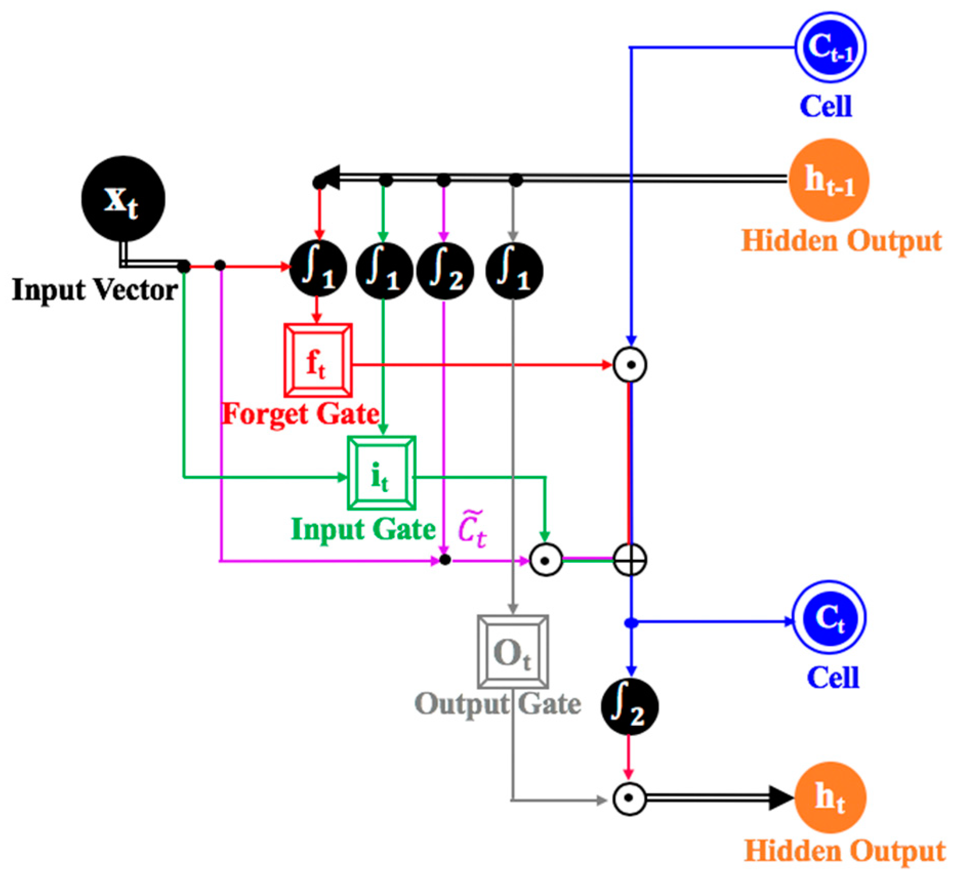
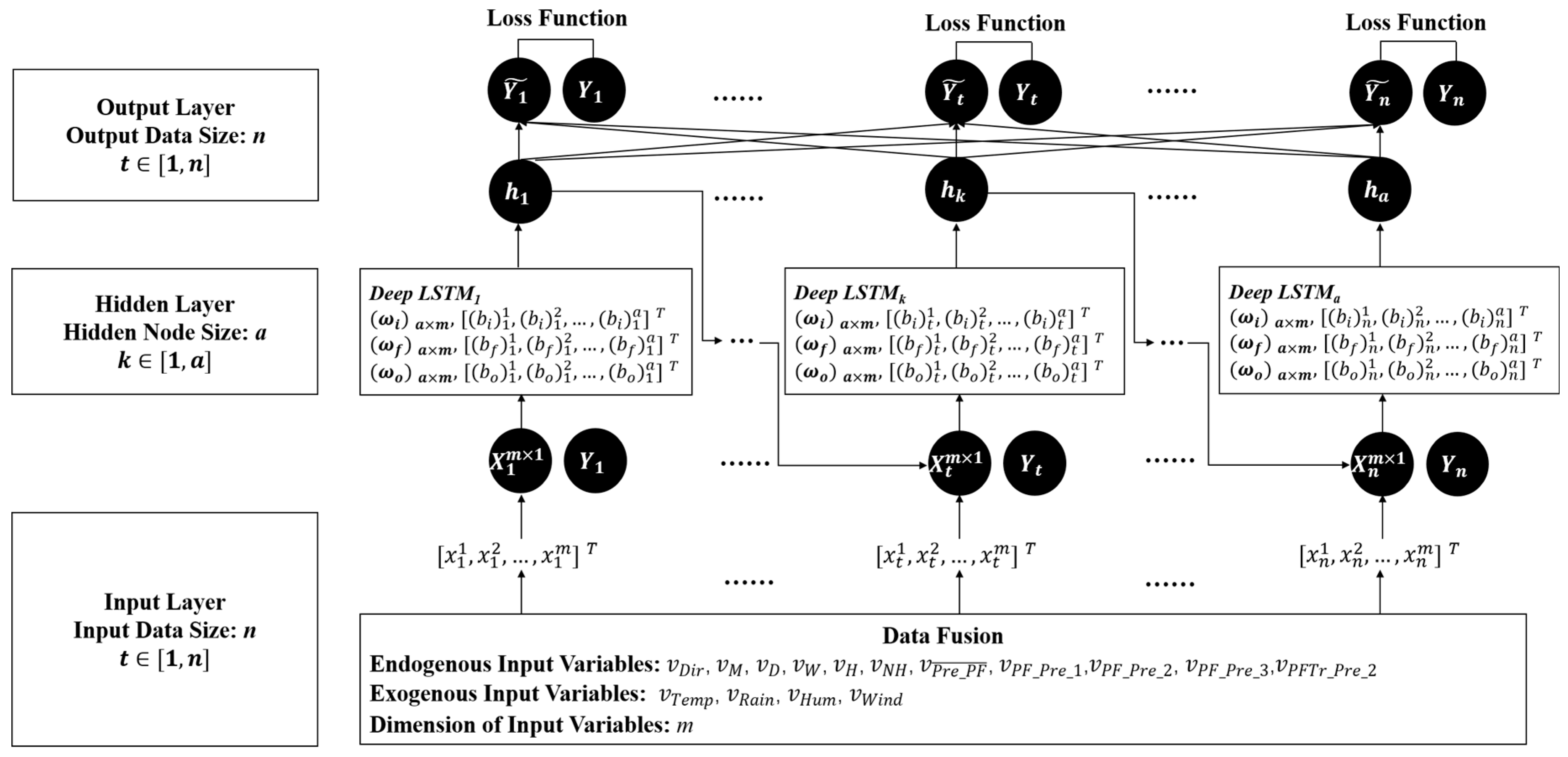
Figure 3 shows the relationship between rainfall and hourly passenger flow on weekdays, weekends, and national holidays. To highlight the impact of rainfall on passenger flow, only the hourly passenger flow on the rainy days is given. The blue bars represent the millimeters of hourly rainfall, and the corresponding hourly passenger flow is marked by the broken black line. To compare the differences between the hourly passenger flow on rainy days, days without rain, and both, we calculated the average hourly passenger flow and marked it with the green dotted line, red dotted line, and yellow dotted line, respectively.

Figure 3a illustrates the impact of rainfall on the inbound passenger flow at different hours on all Mondays during the training dataset. The three peak hours each day are 8:00, 18:00, and 21:00. The red, green, and yellow dotted lines almost overlap with each other. This show that the passenger flow on weekdays is scarcely affected by rain since most trips represent commutes, even if the trips are during the morning and evening peak hours. The lagged impact of rainfall on passenger flow is not obvious after a heavy rain at 6:00.

Figure 3b illustrates the impact of rainfall on the hourly outbound passenger flow at different hours on all Saturdays. The most prominent peak hours are 16:00 to 18:00. These single-peak hours are quite different with the double-peak hours on weekdays. Clearly, the hourly passenger flow on the rainy days is less than the passenger flow on days without rain, as during 6:00–13:00 in Figure 3b. However, if the rain is not heavy, people still execute their travel plans, especially 16:00 to 18:00. This period has the largest passenger volume on weekends.

Figure 3c depicts the impact of rainfall on hourly inbound passenger flow on all national holidays. The most obvious peak hours are 17:00 and 21:00. The difference between the passenger flow on rainy days and on days without rain becomes much greater than in the scenarios in Figure 3b. The impact of rainfall on hourly passenger flow at 8:00, 9:00, 11:00, 15:00, 17:00, 19:00, and 20:00 is greater than the impact at other hours. The flow at 17:00 falls dramatically on rainy days. This shows that the impact of rainfall on hourly passenger flow varies across the morning, noon, and evening hours on national holidays.

In summary, daily trips on national holidays and weekends are more likely to be affected by rainy weather than trips on weekdays, especially on national holidays, findings that are similar to [5]. It is verified that the fluctuation of the black line in Figure 3c is more serious compared to the other two. The possible reason is that travel plans on national holidays and weekends are not necessary, and people are more likely to change or cancel their travel plans due to the rainy days. Although the weather conditions are extremely complex, understanding them is important to improve the hourly passenger flow forecasting results for Taipei Main Station.

3. Methodology

RNN is a class of artificial neural network in which connections between nodes form a directed graph along a temporal sequence. LSTM is a special architecture of RNN, which was first introduced for sequence modeling [28]. It is a useful choice for handling the vanishing gradient problem since it can model long-term dependencies in the data. The vital component in LSTM is a cell. The state of a cell may be changed via control by the input gate, forget gate, and output gate simultaneously. Using this gate mechanism, LSTM has the ability to remove or add extracted hierarchical features and their past states to the cell, which enables LSTM to remember information for long time periods [29]. This state-memory characteristic makes LSTM useful in solving nonlinear time series problems, including a station-level passenger flow forecasting problem.

The architecture of a cell in LSTM is illustrated in Figure 4. Its current input data are typically composed of the input vector X_t at time step t, and the hidden output h_t-1 at time step t-1. The complete work cycle of a cell in LSTM is as follows. First, the three coupled parameters, namely weights and biases (w_i, b_i), (w_f, b_f), and (w_o, b_o), are trained to formulate the nonlinear relationships between the input gate (i_t) and [x_t, h_t-1], the forget gate (f_t) and [x_t, h_t-1], and the output gate (o_t) and [x_t, h_t-1] at time step t, respectively. x_t refers to input data at time step t, and h_t-1 refers to output data in the hidden layer at time step t-1. The formulations of the three gates are defined in Equations (1)–(3). Second, an input squashing vector ($\widetilde{C_t}$) is obtained directly based on Equation (4) without any gate effect at time step t. The new state will then be generated and stored in $C_t$ at time step t under the control of $f_t$, $C_{t-1}$,$i_t$, and $\widetilde{C_t}$, which is shown in Equation (5). This special architecture shows that a cell can add or remove the previous memories stored in $C_{t-1}$ with the control of the forget gate. Finally, the hidden output is obtained based on Equation (6) [30].

$$\mathrm{Input}\mathrm{gate}:i_t={{\displaystyle \int }}_1\left({\omega }_i·\left[x_t,h_{t-1}\right]+b_i\right)$$

(1)

$$\mathrm{Forget}\mathrm{gate}:f_t={{\displaystyle \int }}_1\left({\omega }_f·\left[x_t,h_{t-1}\right]+b_f\right)$$

(2)

$$\mathrm{Output}\mathrm{gate}:O_t={{\displaystyle \int }}_1\left({\omega }_o·\left[x_t,h_{t-1}\right]+b_o\right)$$

(3)

$$\mathrm{Input}\mathrm{squashing}:\widetilde{C_t}={{\displaystyle \int }}_2\left({\omega }_c·\left[x_t,h_{t-1}\right]+b_c\right)$$

(4)

$$\mathrm{Cell}:C_t=f_t\odot C_{t-1}+i_t\odot \widetilde{C_t}$$

(5)

$$\mathrm{Hidden}\mathrm{output}:h_t=O_t\odot [{{\displaystyle \int }}_2\left(C_t\right)]$$

(6)

where ${{\displaystyle \int }}_1$ is the recurrent_activation function and ${{\displaystyle \int }}_2$ is the activation function. In the source codes of the high-level neural network API, such as Keras and Caffe, ${{\displaystyle \int }}_1$ is usually defined as sigmoid [31] or hard sigmoid function [32,33] and ${{\displaystyle \int }}_2$ is defined as tanh function [31,32,33]. $\odot$ refers to Hadamard product [30,34].

The dataflow in a deep LSTM_NN is shown in Figure 5. There is a total of n training examples in the input data. Each set of input data at time step t is defined as an input vector $\left[X_t^{m\times s}\right]$, where m is the number of input variables and s refers to the number of time steps. When modeling, the input variables are assembled as an input vector, namely [$v_{Dir}$, $v_M$, $v_D$, $v_W$, $v_H$, $v_{NH}$, $v_{\overline{Pre\_PF}}$, $v_{PF\_Pre\_1}$, $v_{PF\_Pre\_2}$, $v_{PF\_Pre\_3}$, $v_{PFTr\_Pre\_2}$, $v_{Temp}$, $v_{Rain}$, $v_{Hum}$, $v_{Wind}$], which is the combination of endogenous input variables and exogenous input variables introduced in Section 2.2 and Section 2.3. Since each set of input data contains the variables of the previous 1-hour, 2-hour, and 3-hour passenger flows, we set s=1 as the parameter of time step. This shows that the previous passenger flows at time step (t-1), (t-2), and (t-3) are used as the input variables to forecast the passenger flow at time step t. It is worth noting that the dimension of the input vector [X_t] is changed by multiplying the weight matrixes based on Equations (1)–(4). As a result, the vectors of $i_t,f_t,O_t,\widetilde{C_t},C_t$, and $h_t$ have the same dimensions of a as the size of the hidden nodes and are not equal to the dimension of n in input vector [X_t]. At the output layer, all the hidden outputs are fully connected to obtain $\widetilde{Y_t}$, whose dimension is returned to n. $\widetilde{Y_t}$ is the forecasting result for the passenger flow and $Y_t$ is the actual value of the passenger flow given in the training dataset. This dataflow structure shows that the hourly passenger flow forecasting model can be transformed into a supervised learning problem using a deep LSTM_NN. In other forecast models, $Y_t$ was defined as one of the input variables contained in input vector [X_t] [35] to fit the model, or as [$Y_{t-k},Y_{t-\left(k-1\right)},\dots Y_{t-1}]$, which were a series of previous k-hour passenger flows, to be used as the only input variables to fit the model [36]. In summary, different forecasting tasks should be constructed with the most suitable input variables to obtain the optimized results.

Finally, we calculated the loss l(t) between $Y_t$ and $\widetilde{Y_t}$, where f refers to a loss function in Equation (7). Equation (8) was used to minimize the error between $Y$ and $\tilde{Y}$ over an entire sequence of length T using one of the state-of-the-art optimization algorithms [37]. To deeply and rapidly extract the relationship between the input variables and passenger flow, the deep structural LSTM_NN was applied in the experiment.

$$l\left(t\right)=f\left(Y_t-\widetilde{Y_t}\right)$$

(7)

$$\min \left(L\right)=\min [{\displaystyle \sum }_{t=1}^{T}l\left(t\right)]=\frac{\partial L}{\partial w}$$

(8)

4. Experimental Results and Discussion

4.1. Data Specification

As discussed in Section 2, the considered input variables and their encoded values are listed in

Table 2. Information on the input variables.

No.	Input Variables	Encoded Values	Descriptions
1	$v_{Dir}$	0,1	0: inbound; 1: outbound
2	$v_M$	1–12	January–December
3	$v_D$	1–31	31 days per month
4	$v_W$	1–7	Monday–Sunday
5	$v_H$	0–23	24 hours per day
6	$v_{NH}$	Table 3
7	$v_{\overline{Pre\_PF}}$	calculated	(1) Normal days: The average value of hourly passenger flow on all non-national holidays; (2) National holidays: The average value of hourly passenger flow on all national holidays.
8	$v_{PF\_Pre\_1}$	actual	Previous 1-hour passenger flow
9	$v_{PF\_Pre\_2}$	actual	Previous 2-hour passenger flow
10	$v_{PF\_Pre\_3}$	actual	Previous 3-hour passenger flow
11	$v_{PFTr\_Pre\_2}$	calculated	(Previous 1-hour passenger flow)-(Previous 2-hour passenger flow)
12	$v_{Temp}$	actual	Actual hourly atmospheric temperature (°C)
13	$v_{Rain}$	actual	Actual hourly rainfall (mm)
14	$v_{Hum}$	actual	Actual hourly relative humidity ($\%)$
15	$v_{Wind}$	actual	Actual hourly average wind speed (mile/second)
16	$v_{PF}^{*}$	actual	Actual hourly passenger flow

. The traditional input variables labeled No. 1–11 were assembled with different weather variables labeled No. 12–15. These assembled input variables are defined as the input vector [X_t]. Hourly passenger flow ($v_{PF}^{*}$) is the target variable for forecasting (Y_t). Table 2 lists the descriptions of the input variables.$v_{NH}$ has been encoded as a two-digit figure, shown in

Table 3. Durations of the national holidays and their encoded values.

National Holiday	Order	Durations	Encoded Values
New Year’s Day	1	About 3 or 4 days	11, 12, 13, 19
Lunar New Year’s Day	2	About 6–9 days	21–29
Peace Memorial Day	3	About 3 days	31, 32, 39
Tomb-Sweeping Day	4	About 3 or 4 days	41, 42, 43, 49
Dragon Boat Day	5	About 3 or 4 days	51, 52, 53, 59
Mid-Autumn Day	6	About 3 or 4 days	61, 62, 63, 69
National Day	7	About 3 days	71, 72, 79

. The encoded values of input variables labeled No. 1–11 are described in [26].

In the experiment, we developed many LSTM NN-based models for hourly passenger flow forecasting with Keras in Python. All training data and testing data were normalized and shuffled before training and testing.

Root mean square error (RMSE) and mean absolute percentage error (MAPE) are the two most commonly used criteria to evaluate the performance of a passenger flow forecasting model [26]. Thus, RMSE and MAPE in Equations (9) and (10) were used to evaluate the performance of the forecasting model.

The lower the value in RMSE or MAPE, the better the performance.

$$RMSE=\sqrt{\frac{1}{n}{\displaystyle \sum }_{t=1}^n{\left|{(Y_r)}_t-{(Y_f)}_t\right|}^2}$$

(9)

$$MAPE=\frac{1}{n}{{\displaystyle \sum }}_{t=1}^n\frac{\left|{(Y_r)}_t-{(Y_f)}_t\right|}{{\left(Y_r\right)}_t}$$

(10)

4.2. Results of not Using any Weather Variables

To evaluate the forecasting performance of the deep LSTM_NN, we first compared the experimental results using the deep LSTM_NN, one-layer LSTM_NN, and RF, respectively. Without adding any weather variable, the optimized combination of traditional input variables ($v_{Dir}$,$v_M$, $v_D$,$v_W$,$v_H$,$v_{NH}$,$v_{\overline{Pre\_PF}}$,$v_{PF\_Pre\_1}$,$v_{PF\_Pre\_2}$, $v_{PF\_Pre\_3}$,$v_{PFTr\_Pre\_2}$) used in [26] were implemented in this section first.

The tuning parameters for the deep LSTM_NN and one-layer LSTM_NN are shown in

Table 4. Tuning parameters in the deep LSTM_NN and one-layer LSTM_NN.

No.	Parameters	Values
1	epochs	{500, 1000, 1500, 2000, 2500, 3000, 3500, 4000, 4500, 5000}
2	batch size	{32, 64, 128, 256, 512}
3	activation	{relu, tanh, sigmoid}
4	recurrent_activation	{relu, tanh, sigmoid, hard_sigmoid}
5	learning rate	{0.001, 0.002, 0.003, 0.004, 0.005}
6	hidden nodes	{(50), (100), (200), (250), (256,128,64,10), (256,128,64,32), (256,128,64,32,10), (256,128,64), (256,256,256), (258,126)}
7	number of hidden layers	{1, 2, 3, 4}
8	optimizer	{RMSprop, adam, adamax, adagrad, SGD}
9	dropout	{0.05, 0.1, 0.2, 0.3, 0.4, 0.5, 0.6, 0.7, 0.8, 0.9}
10	momentum	{0, 0.1, 0.2, 0.3, 0.4, 0.5, 0.6, 0.7, 0.8, 0.9}

. The best tuning results of parameters for the deep LSTM_NN, one-layer LSTM_NN, and RF are given in

Table 5. Best tuning results of the parameters in the deep LSTM_NN, one-layer LSTM_NN, and RF.

No.	Parameters	Best Tuning Results
		Deep LSTM_NN	One-layer LSTM_NN	RF
1	epochs	1000	3500	✕
2	batch size	256	128	✕
3	activation	tanh	relu	✕
4	recurrent_activation	hard_sigmoid	hard_sigmoid	✕
5	learning rate	0.001	0.001	✕
6	hidden nodes	(256,128,64)	(100)	✕
7	number of hidden layers	3	1	✕
8	optimizer	adam	adam	✕
9	dropout	0.05	0.05	✕
10	momentum	0.9	0	✕
11	max_features	✕	✕	3
12	n_estimators	✕	✕	6500
Evaluation Criteria	RMSE	490.77	517.63	538.75
	MAPE	0.0547	0.0629	0.0555

. As shown in Table 5 and the experimental results in [26], the three-layer LSTM_NN with RMSE = 490.77 and MAPE = 0.0547 has the better forecasting results than the one-layer LSTM_NN and RF. The experimental results verify that the deep LSTM_NN enables more accurate results than either one-layer LSTM_NN or RF.

4.3. Results of Using Weather Variables

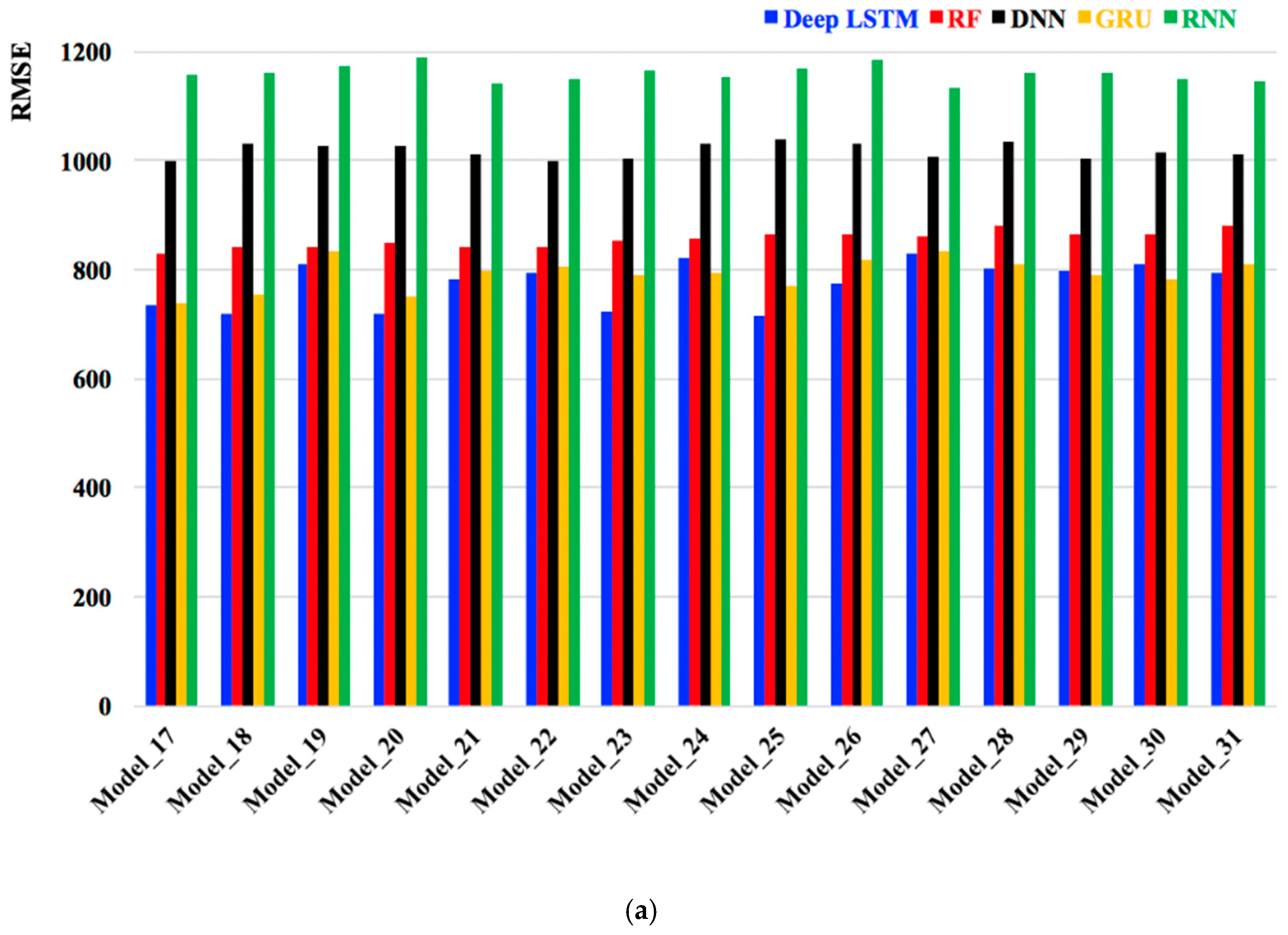
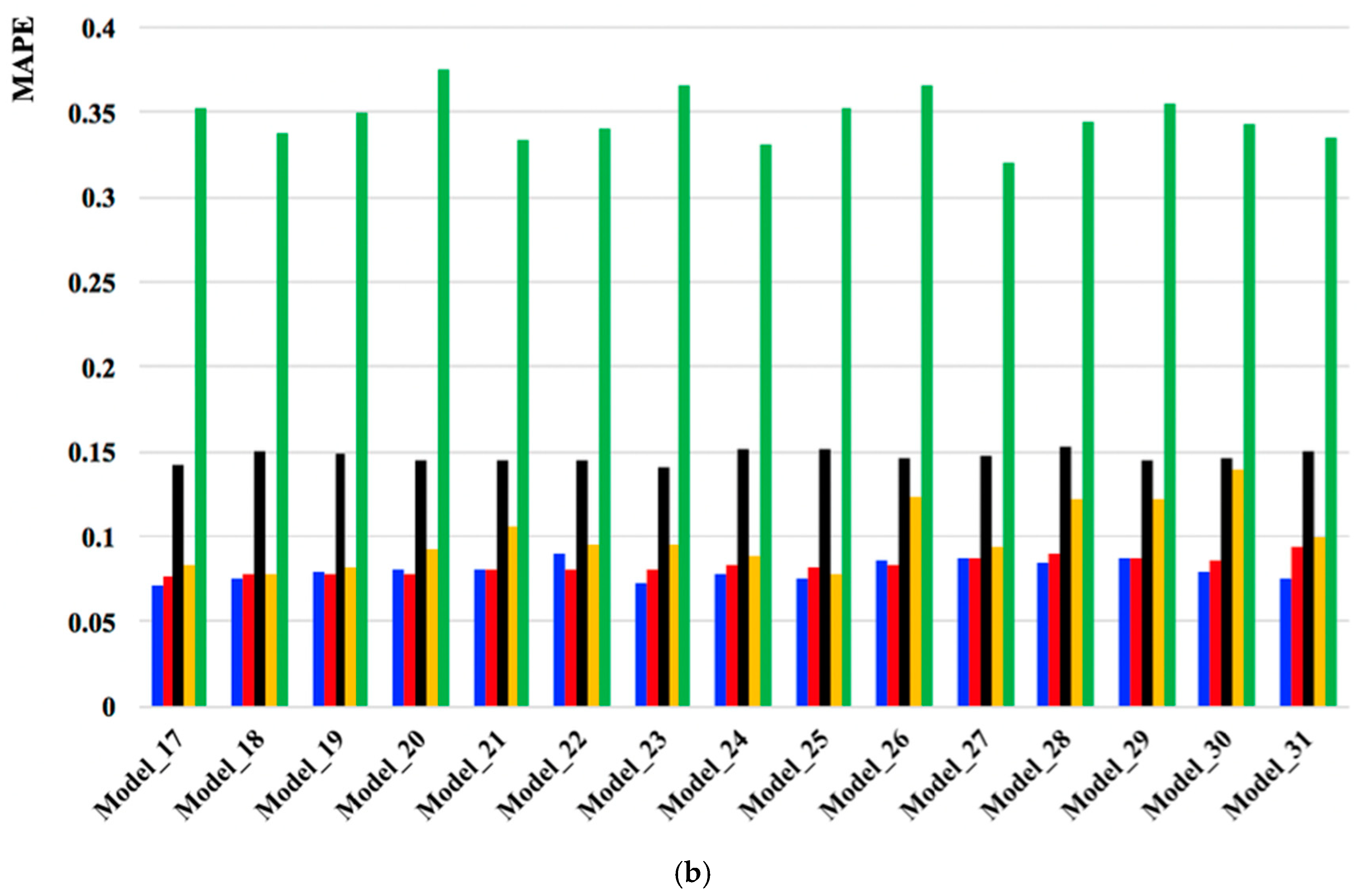
As shown in Figure 3, the passenger flow on rainy days is quite different than on days without any rain. Adverse weather conditions may have great impacts on daily commutes. Thus, making a more accurate passenger flow forecast on rainy days is useful. The training data and testing data used for rainy days are shown in

Table 6. Description of training dataset and testing dataset on rainy days.

Dataset	Total Examples	Raining Examples	Ratio (Raining Examples/Total Examples)
Training dataset	14,164	1748	12.34%
Testing dataset	5898	524	11.26%

. To comprehensively discuss the different combinations of weather variables on passenger flow forecasting, 31 models were built and categorized as three groups using the proposed deep LSTM_NN on rainy days. Model_1 in Group_1 was built without using any weather variable, in order to make a comparison with the models using weather variables. Models 2–16 in Group_2 were built with different combinations of current hourly weather variables, and Models 17–31 in Group_3 were built with different combinations of previous one-hour weather variables.

The tuning parameters of the proposed deep LSTM_NN are shown in Table 4. The best grid result is a group of the following parameters: (1) epochs: 4500; (2) batch_size: 256; (3) activation function (${{\displaystyle \int }}_1$): tanh; (4) recurrent_activation function (${{\displaystyle \int }}_2)$: hard_sigmoid; (5) learning rate: 0.003; (6) hidden nodes: (256, 128, 64); (7) number of hidden layers: 3; (8) optimizer: adam; (9) dropout: 0.5; and (10) momentum = 0.9. The used loss function is mean_squared_error.

Table 7. Results of Models 1 and 2–16.

Models	Input Variables					Deep LSTM_NN
	Optimized Traditional Input Variables	${\mathit{v}}_{\mathit{T}\mathit{e}\mathit{m}\mathit{p}}$	${\mathit{v}}_{\mathit{R}\mathit{a}\mathit{i}\mathit{n}}$	${\mathit{v}}_{\mathit{H}\mathit{u}\mathit{m}}$	${\mathit{v}}_{\mathit{W}\mathit{i}\mathit{n}\mathit{d}}$	RMSE	MAPE
1	•	✕	✕	✕	✕	753.88	0.0741
2	•	•	✕	✕	✕	754.76	0.0730
3	•	✕	•	✕	✕	726.76	0.0760
4	•	✕	✕	•	✕	770.12	0.0732
5	•	✕	✕	✕	•	745.83	0.0815
6	•	•	•	✕	✕	805.87	0.0818
7	•	•	✕	•	✕	771.99	0.0846
8	•	•	✕	✕	•	748.08	0.0757
9	•	✕	•	•	✕	820.02	0.0787
10	•	✕	•	✕	•	787.60	0.0864
11	•	✕	✕	•	•	793.76	0.0760
12	•	•	•	•	✕	829.60	0.0987
13	•	✕	•	•	•	855.64	0.0801
14	•	•	✕	•	•	785.41	0.1001
15	•	•	•	✕	•	804.82	0.0734
16	•	•	•	•	•	823.14	0.0849

•: The input variable has been used in the corresponding model; ✕: The input variable hasn’t been used in the corresponding model.

shows the experimental results of Models 1–16. Unfortunately, both RMSE and MAPE of the forecast performance in Models 6, 7, and 9–16 was not improved by adding the current hourly weather variables, especially for the combined weather variables as the inputs in comparison with RMSE and MAPE in Model_1. However, adding a single weather variable, such as $v_{Temp}$(MAPE in Model_2), $v_{Rain }$(RMSE in Model_3),$v_{Hum}$(MAPE in Model_4), or $v_{Wind}$ (RMSE in Model_5), and the combined weather variable of $v_{Temp}$ and $v_{Wind}$ (RMSE in Model_8), can improve the forecasting results slightly.

To understand the socio-psychological aspects of the travel behavior of metro passengers, we suppose that individuals may give up their plans to go out if it is raining outside, especially during non-working hours. In this case, the previous one-hour weather variables may be the more important inputs for forecasting tasks than the current hourly weather variables. Therefore, Models 17-31 were built by the various combinations of the previous one-hour weather variables, in order to improve the results of forecasts made using no weather variable on rainy days.

Table 8. Results of Models 1 and 17–31.

Models	Input Variables					Deep LSTM_NN
	Optimized Traditional Input Variables	${\mathit{v}}_{\mathit{T}\mathit{e}\mathit{m}\mathit{p}\_\mathit{P}\mathit{r}\mathit{e}\_1}$	${\mathit{v}}_{\mathit{R}\mathit{a}\mathit{i}\mathit{n}\_\mathit{P}\mathit{r}\mathit{e}\_1}$	${\mathit{v}}_{\mathit{H}\mathit{u}\mathit{m}\_\mathit{P}\mathit{r}\mathit{e}\_1}$	${\mathit{v}}_{\mathit{W}\mathit{i}\mathit{n}\mathit{d}\_\mathit{P}\mathit{r}\mathit{e}\_1}$	RMSE	MAPE
1	•	✕	✕	✕	✕	753.88	0.0741
17	•	•	✕	✕	✕	735.79	0.0711
18	•	✕	•	✕	✕	718.83	0.0752
19	•	✕	✕	•	✕	809.57	0.0793
20	•	✕	✕	✕	•	718.83	0.0813
21	•	•	•	✕	✕	782.14	0.0806
22	•	•	✕	•	✕	794.34	0.0902
23	•	•	✕	✕	•	722.79	0.0734
24	•	✕	•	•	✕	823.00	0.0780
25	•	✕	•	✕	•	713.60	0.0757
26	•	✕	✕	•	•	773.20	0.0863
27	•	•	•	•	✕	831.89	0.0873
28	•	✕	•	•	•	802.04	0.0852
29	•	•	✕	•	•	796.50	0.0873
30	•	•	•	✕	•	810.28	0.0798
31	•	•	•	•	•	794.13	0.0758

•: The input variable has been used in the corresponding model; ✕: The input variable hasn’t been used in the corresponding model.

shows the experimental results for Models 1 and 17–31.

As shown in Table 8, both RMSE and MAPE in Models 17 and 23 are lower than Model_1. The better experimental results indicate that using the previous one-hour weather data as the input variable can improve the forecasting results of passenger flow on rainy days. These results match our assumptions about travelers’ psychology. Using the combined weather variables of $v_{Temp\_Pre\_1}$ and $v_{Wind\_Pre\_1}$ in Model_23 results in more accurate forecasts than Model_1 by RMSE. The results indicate that travelers may cancel their travel plans if the weather is cold and windy on rainy days. These two previous one-hour weather variables, namely $v_{Temp\_Pre\_1}$ and $v_{Wind\_Pre\_1}$, may be helpful in developing a more powerful forecast model on rainy days. These encouraging results demonstrate that understanding the socio-psychological aspects of the travel behavior of metro passengers is truly important to apply appropriate weather data for developing a more powerful passenger flow forecasting model.

4.4. Comparisons

To better analyze the forecasting performance of the deep LSTM_NN, four methods were selected for comparisons, namely RF [38], deep neural network (DNN) [18], RNN [20], and GRU [39]. We have discussed the optimized combination of the endogenous input variables using RF in our previous study [26], and the impacts of added weather variables on passenger flow forecasting have been further studied. Therefore, RF was further selected as one of the important comparative methods. Furthermore, the other three neural networks (DNN, RNN, and GRU) are the typical artificial intelligence algorithms that are successfully applied to many different forecasting tasks. The parameters of n_estimators and max_features in RF were chosen with the same values as in Section 4.2. To make an equal comparison among different neural network models, the parameters used in DNN, RNN, and GRU were the same as in the deep LSTM_NN, described in Section 4.3. The training samples and input variables used in the above four methods were identical to those used in Models 17–31. Figure 6 shows the RMSE and MAPE of the forecasting results in the five methods. The deep LSTM_NN is better than the other four methods when incorporating previous one-hour weather variables as the inputs in most scenarios. These results verify that the deep LSTM_NN can better extract and represent the deep variables of passenger flow embedded in the training dataset. It is a more powerful method for time series forecasting problems.

5. Conclusions

Inspired by the close relationship between weather conditions and passenger flow forecasting, a detailed experimental analysis of the impacts of weather variables on passenger flow forecasting using a deep LSTM_NN was conceived. The experimental results show that the previous one-hour temperature ($v_{Temp\_Pre\_1}$) and previous one-hour wind speed ($v_{Wind\_Pre\_1}$), especially $v_{Temp\_Pre\_1}$, are the two most important weather variables for passenger flow forecasting on rainy days. Compared to the other four algorithms, the deep LSTM_NN is a more powerful method to make the more accurate forecasts when suitable weather variables are included. Since the previous one-hour weather data are not difficult to obtain, the model developed herein for short-term metro passenger flow forecasting may be performed in practical applications.

The majority of weather data present general variations, which do not have much impact on passengers’ daily commuting, even in the case of heavy rain. This indicates that adding current hourly weather data to build a forecasting model may not be helpful in improving the forecasting results, because the weather data are more likely to be noisy data. The experimental results in Table 7 support this assumption. Fortunately, instead of using current hourly weather data, we used the previous one-hour weather data to develop the model, which yields the better results. These encouraging results demonstrate that understanding the socio-psychological aspects of the travel behavior of metro passengers is truly important to apply appropriate weather data for developing a more powerful passenger flow forecasting model. This special strategy is creative and helpful in data modeling.

Because the testing data ran from November 2016 to March 2017, the weather during this period is relatively colder and drier. The experimental results can only verify that the proposed model can forecast passenger flows more accurately when weather conditions are broadly similar. As shown in Table 6, the training and testing examples are not rich enough for forecasting passenger flows on rainy days. In the future, we will collect more data to perform these forecasting tasks and further verify the results using days with adverse weather, such as typhoons, heavy rains, or high winds, and for weekends and national holidays with rainy days. In addition, because the weather conditions shift randomly at the hour-level, clustering methods may be used to group the training data and testing data based on different weather conditions before developing a forecasting model. As another possibility of exploring the impact of weather on passenger flow forecasting, the addition of seasonal variations or outdoor thermal comfort may also have an essential impact on travel behavior at specific traffic nodes [40]. All these represent productive directions for our future research.

References

1. Wang, J.Z.; Kong, X.J.; Zhao, W.H.; Tolba, A.; Al-Makhadmeh, Z.; Feng, X. STLoyal: A spatio-temporal loyalty-based model for subway passenger flow prediction. IEEE Access 2018, 6, 47461–47471. [Google Scholar]
2. Zhao, J.J.; Zhang, F.; Tu, L.; Xu, C.Z.; Shen, D.Y.S.; Tian, C.; Li, X.Y.; Li, Z.X. Estimation of passenger route choice pattern using smart card data for complex metro systems. IEEE Transp. Intell. Transp. Syst. 2017, 18, 790–801. [Google Scholar] [CrossRef]
3. Yan, D.F.; Wang, J. Subway passenger flow forecasting with multi-station and external factors. IEEE Access 2019, 7, 57415–57423. [Google Scholar]
4. Saneinejad, S.; Roorda, M.J.; Kennedy, C. Modelling the impact of weather conditions on active transportation travel behavior. Transp. Res. D Transp. Environ. 2012, 17, 129–137. [Google Scholar] [CrossRef] [Green Version]
5. Singhal, A.; Kamga, C.; Yazici, A. Imapct of weather on urban transit ridership. Transp. Res. A Pol. Prac. 2014, 69, 379–391. [Google Scholar] [CrossRef]
6. Hao, S.; Lee, D.; Zhao, D. Sequence to sequence learning with attention mechanism for short- term passenger flow prediction in large-scale metro system. Transp. Res. C Emerg. Technol. 2019, 107, 287–300. [Google Scholar] [CrossRef]
7. Tao, S.; Corcoran, J.; Rowe, F.; Hickman, M. To travel or not to travel: ‘Weather’ is the question. Modelling the effect of local weather conditions on bus ridership. Transp. Res. C Emerg. Technol. 2018, 86, 147–167. [Google Scholar] [CrossRef]
8. Xu, M.L.; Fu, X.; Tang, J.Y.; Liu, Z.Y. Effects of weather factors on the spatial and temporal distributions of metro passenger flows: An empirical study based on smart card data. Prog. Geogr. 2020, 39, 45–55. [Google Scholar] [CrossRef]
9. Ke, J.T.; Zheng, H.Y.; Yang, H.; Chen, X.Q. Short-term forecasting of passenger demand under on-demand ride services: A spatio-temporal deep learning approach. Transp. Res. Res. C Emerg. Technol. 2017, 85, 591–608. [Google Scholar] [CrossRef]
10. Tang, L.; Zhao, Y.; Cabrera, J.; Ma, J.; Tsui, K. Forecasting short-term passenger flow: An empirical study on Shenzhen metro. IEEE Transp. Intell. Transp. Syst. 2019, 20, 3613–3622. [Google Scholar] [CrossRef]
11. Chen, W.Y.; Pan, X.; Fang, X.P. Short-term prediction of passenger flow on bus routes based on K-means clustering combination models. J. S. China Univ. Technol. (Nat. Sci.) 2019, 47, 83–89, 113. [Google Scholar]
12. Liu, X.T.; Huang, X.L.; Xie, B.L. A model of short-term forecast of passenger flow of buses based on SVM-KNN under rainy conditions. J. Transp. Inf. Saf. 2018, 36, 117–123. [Google Scholar]
13. Li, M.; Li, J.; Wei, Z.J.; Wang, S.D.; Chen, L.J. Short-term passenger flow forecasting at subway station based on deep learning LSTM structure. Urban Mass Trans. 2018, 42–46, 77. [Google Scholar]
14. Wan, H.; Guo, S.; Yin, K.; Liang, X.; Lin, Y. CTS-LSTM: LSTM-based neural networks for correlated time series prediction. Knowledge-Based Syst. 2020, 191, 1–10. [Google Scholar] [CrossRef]
15. Stover, V.W.; Nygaard, N. The impact of weather on bus ridership in pierce county, Washington. J. Pub. Transp. 2012, 15, 95–110. [Google Scholar] [CrossRef] [Green Version]
16. Bocker, L.; Dijst, M.; Prillwitz, J. Impact of everyday weather on individual daily travel behaviours in perspective: A literature review. Transp. Rev. 2013, 33, 71–91. [Google Scholar] [CrossRef]
17. Liu, C.X.; Susilo, Y.O.; Karlström, A. The influence of weather characteristics variability on individual’s travel mode choice in different seasons and regions in Sweden. Transp. Policy 2015, 41, 147–158. [Google Scholar] [CrossRef]
18. Wang, Y.; Zhang, D.; Liu, Y.; Dai, B.; Lee, L. Enhancing transportation systems via deep learning: A survey. Transp. Res. C Emerg. Technol. 2019, 99, 144–163. [Google Scholar] [CrossRef]
19. Schmidhuber, J. Deep learning in neural networks: An overview. Neural Netw. 2015, 61, 85–117. [Google Scholar] [CrossRef] [Green Version]
20. Ding, Y.X.; LI, Z.; Zhang, C.D.; Ma, J. Correlation filtered spatial-temporal long short-term memory model.
21. Li, X.Y.; Li, J.L.; Qu, Y.Z.; He, D. Gear pitting fault diagnosis using integrated CNN and GRU network with both Vibration and Acoustic Emission Signals. Science 2019, 9, 4. [Google Scholar] [CrossRef] [Green Version]
22. Jozefowicz, R.; Zaremba, W.; Sutskever, I. An Empirical Exploration of Recurrent Network Architectures; JMLR: Lille, France, 2015; pp. 2342–2350. [Google Scholar]
23. Zhao, Z.; Chen, W.H.; Wu, X.M.; Chen, C.Y.; Liu, J.M. LSTM network: A deep learning approach for short-term traffic forecast. IET Intell. Transp. Syst. 2017, 11, 68–75. [Google Scholar] [CrossRef] [Green Version]
24. Wang, X.; Jiang, R.; Li, L.; Lin, Y.L.; Zheng, X.H.; Wang, F.Y. Capturing car-following behaviors by deep learning. IEEE Transp. Intell. Transp. Syst. 2018, 19, 910–920. [Google Scholar] [CrossRef]
25. Taipei Open Government. Hourly Inbound and Outbound Passenger Flow in Taipei Metro. Available online: https://data.taipei/dataset/detail/metadata?id=63f31c7e-7fc3-418b-bd82-b95158755b4d (accessed on 1 January 2019).
26. Liu, L.J.; Chen, R.C.; Zhao, Q.F.; Zhu, S.Z. Applying a multistage of input feature combination to random forest for improving MRT passenger flow prediction. J. Ambient Intell. Humaniz. Comput. 2019, 10, 4515–4532. [Google Scholar] [CrossRef]
27. Taiwan Environmental Protection Administration. Annual Weather in Taipei. Available online: https://taqm.epa.gov.tw/taqm/tw/YearlyDataDownload.aspx. (accessed on 31 December 2018).
28. Hochreiter, S.; Schmidhuber, J. Long short-term memory. Neural Comput. 1997, 9, 1735–1780. [Google Scholar] [CrossRef]
29. Ott, J.; Lin, Z.H.; Zhang, Y.; Liu, S.C.; Bengio, Y.S. Recurrent neural. networks with limited numerical precision. arXiv 2017, arXiv:1608.06902v2. [Google Scholar]
30. Wu, Y.H.; Zhang, S.Z.; Zhang, Y.; Bengio, Y.S.; Salakhutdinov, R. On Multiplicative Integration with Recurrent Neural Networks; NIPS: Barcelona, Spain, 2016; pp. 1–9. [Google Scholar]
31. Donahue, J. LSTM Layer and LSTM Unit Layer, with Tests. Available online: https://github.com/BVLC/caffe/blob/master/include/caffe/layers/lstm_layer.hpp (accessed on 2 June 2016).
32. Allaire, J. Package ‘Keras’. Available online: https://cran.r-project.org/web/packages/keras/keras.pdf (accessed on 22 November 2018).
33. Meudec, R. Identity Initializer with Zero Padding. Available online: https://github.com/keras-team/keras/blob/master/keras/layers/recurrent.py#L900 (accessed on 5 January 2019).
34. Koutaki, G.; Shirai, K.; Ambai, M. Hadamard Coding for Supervised. Discrete Hashing. IEEE Trans. Image. Process. 2018, 27, 5378–5392. [Google Scholar] [CrossRef]
35. Brownlee, J. Multivariate Time Series Forecasting with LSTMs in Keras. Available online: https://machinelearningmastery.com/multivariate-time-series-forecasting-lstms-keras/ (accessed on 14 August 2017).
36. Resuly. Using RNN to Forecast for the Time Series Sequence with Keras. Available online: http://resuly.me/2017/08/16/keras-rnn-tutorial/ (accessed on 16 August 2017).
37. Kingma, D.P.; Ba, J.L. Adam: A method for stochastic optimization. arXiv 2017, arXiv:1412.6980v9. [Google Scholar]
38. Breiman, L. Random forests. Mach. Learn. 2011, 45, 5–32. [Google Scholar] [CrossRef] [Green Version]
39. Chung, J.Y.; Gulcehre, C.; Cho, K.H.; Bengio, Y.S. Empirical evaluation of gated recurrent neural networks on sequence modeling. arXiv 2014, arXiv:1412.3555v1. [Google Scholar]
40. Nikolopoulou, M. Outdoor thermal comfort. Front. Biosci. 2011, S3, 1552–1568. [Google Scholar] [CrossRef]
Figure 1. Top 10 stations with the highest average daily passenger flow in the Taipei MRT.
Applsci 10 02962 g001
Figure 2. Annual weather conditions from 1 November 2015 to 31 October 2016 around Taipei Main Station.
Applsci 10 02962 g002
Figure 3. Impact of rainfall on hourly passenger flow in the training dataset. (a) Impact of rainfall on hourly inbound passenger flow on all Mondays in the training dataset. (b) Impact of rainfall on hourly outbound passenger flow on all Saturdays in the training dataset. (c) Impact of rainfall on hourly inbound passenger flow on all national holidays in the training dataset.
Applsci 10 02962 g003aApplsci 10 02962 g003b
Figure 4. A cell in long short-term memory (LSTM).
Applsci 10 02962 g004
Figure 5. Dataflow in a deep long short-term memory neural network (LSTM_NN).
Applsci 10 02962 g005
Figure 6. Comparison of forecasting results in the five methods. (a) Root mean square error (RMSE) of forecasting results in the five methods. (b) Mean absolute percentage error (MAPE) of forecasting results in the five methods.
Applsci 10 02962 g006aApplsci 10 02962 g006b