FCN-Based 3D Reconstruction with Multi-Source Photometric Stereo


Abstract
1. Introduction
2. Materials and Methods
2.1. The Multi-Source Photometric Stereo
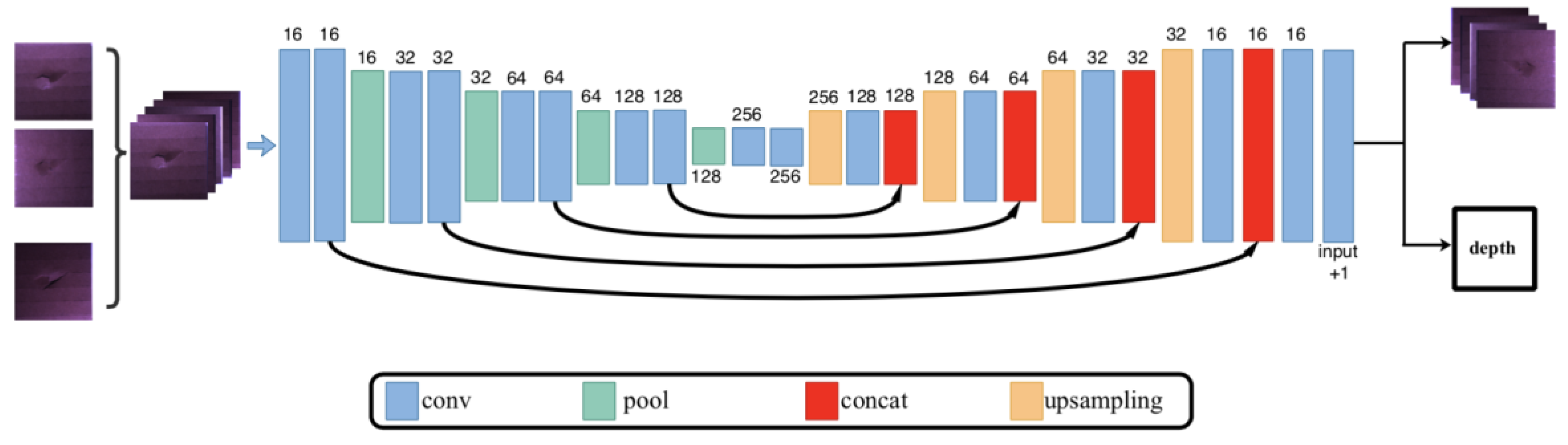
2.2. Network Architecture
2.3. Loss Function
2.4. Dataset
2.4.1. The Real-World Dataset
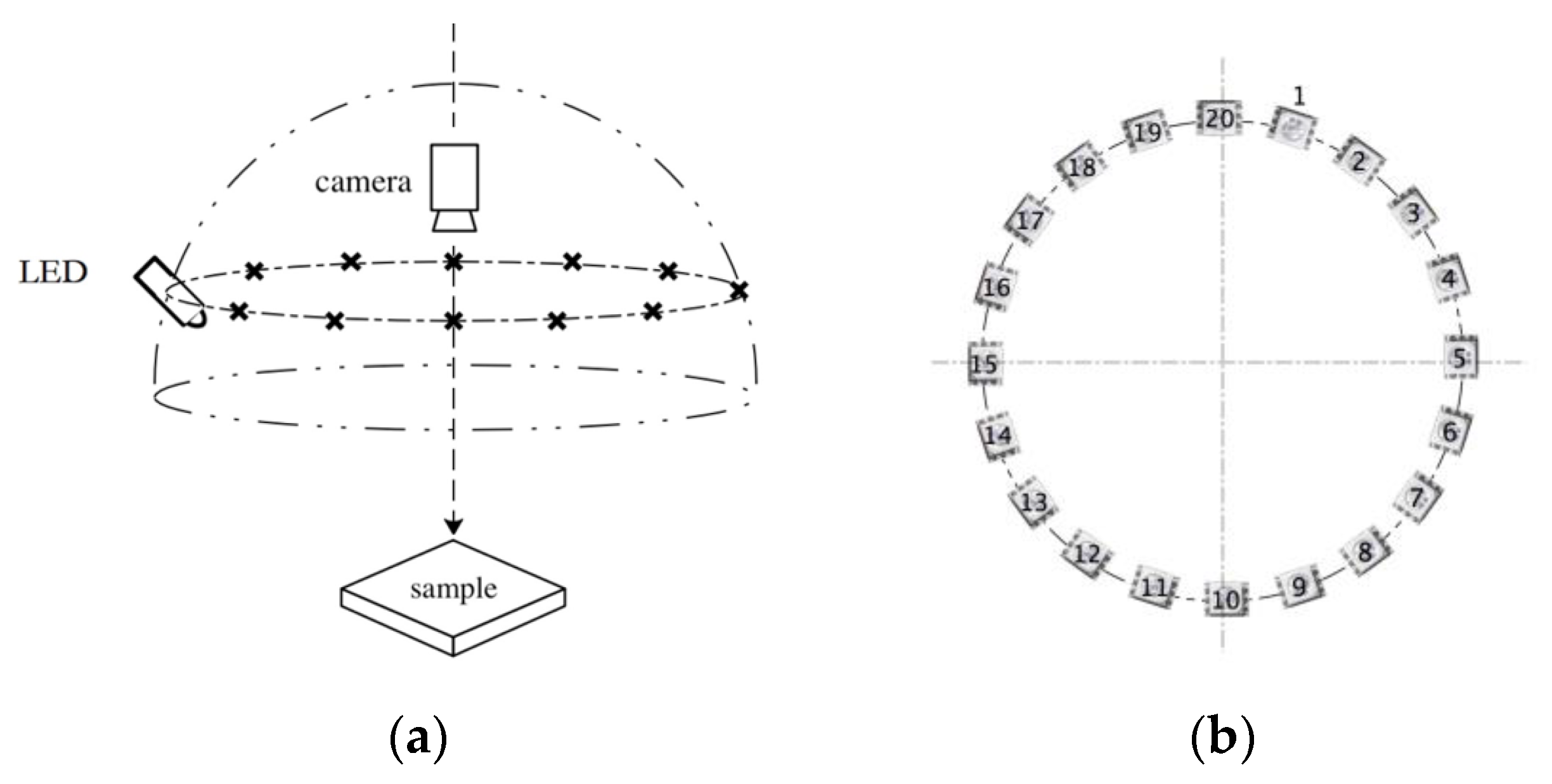
2.4.2. The Photometric Acquisition Setup
2.4.3. Data Capture
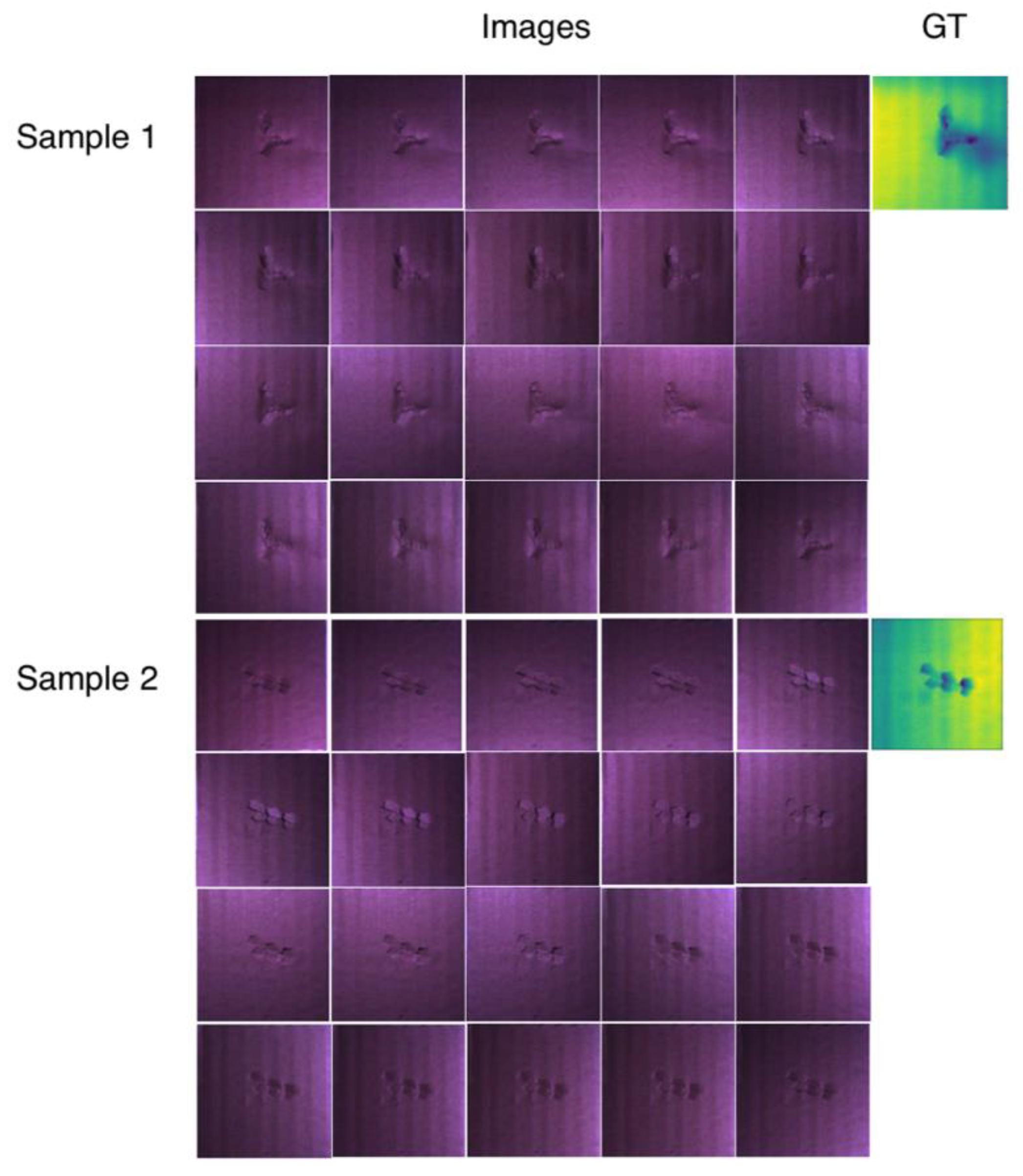
3. Results
3.1. Implementation Details
3.2. Error Metrics
- 1.
- root mean squared error(rms)
- 2.
- average relative error(rel)
- 3.
- threshold accuracy()
4. Discussion
4.1. Compared with the Classic Multi-Source PS
4.2. Effectiveness of the New Regularization Constraints
5. Conclusions
Author Contributions
Funding
Conflicts of Interest
References
- Horn, B.K.P. Shape from Shading: A Method for Obtaining the Shape of a Smooth Opaque Object from One View. Ph.D. Thesis, Department of Electrical Engineering, MIT, Cambridge, UK, 1970. [Google Scholar]
- Woodham, R.J. Photometric method for determining surface orientation from multiple images. Opt. Eng. 1980, 19, 139–144. [Google Scholar] [CrossRef]
- Xu, K.; Wang, L.; Xiang, J.; Zhou, P. Three-dimensional defect detection method of metal surface based on multi-point light source. China Sci. 2017, 12, 420–424. (In Chinese) [Google Scholar]
- Sun, J.; Smith, M.; Smith, L.; Midha, S.; Bamber, J. Object surface recovery using a multi-light photometric stereo technique for non-Lambertian surfaces subject to shadows and specularities. Image Vis. Comput. 2007, 25, 1050–1057. [Google Scholar] [CrossRef]
- Wang, L.; Xu, K.; Zhou, P.; Yang, C. Photometric stereo fast 3D surface reconstruction algorithm using multi-scale wavelet transform. J. Comput. -Aided Des. Comput. Graph. 2017, 29, 124–129. (In Chinese) [Google Scholar]
- Cho, D.; Matsushita, Y.; Tai, Y.W.; Kweon, I. Photometric Stereo Under Non-uniform Light Intensities and Exposures. In Proceedings of the European Conference on Computer Vision, Amsterdam, The Netherlands, 8–16 October 2016. [Google Scholar]
- Hertzmann, A.; Seitz, S.M. Example-based photometric stereo: Shape reconstruction with general, varying BRDFs. IEEE Trans. Pattern Anal. Mach. Intell. 2005, 27, 1254–1264. [Google Scholar] [CrossRef] [PubMed]
- Li, X.; Dong, Y.; Peers, P.; Tong, X. Synthesizing 3D Shapes from Silhouette Image Collections using Multi-projection Generative Adversarial Networks. In Proceedings of the IEEE Conference on Computer Vision and Pattern Recognition, Long Beach, CA, USA, 16–20 June 2019; pp. 5535–5544. [Google Scholar]
- Sun, C.Y.; Zou, Q.F.; Tong, X.; Liu, Y. Learning Adaptive Hierarchical Cuboid Abstractions of 3D Shape Collections. ACM Trans. Graph. 2019, 38, 1–13. [Google Scholar] [CrossRef]
- Tang, J.; Han, X.; Pan, J.; Jia, K.; Tong, X. A Skeleton-bridged Deep Learning Approach for Generating Meshes of Complex Topologies from Single RGB Images. In Proceedings of the IEEE Conference on Computer Vision and Pattern Recognition, Long Beach, CA, USA, 16–20 June 2019; pp. 4541–4550. [Google Scholar]
- Wu, Z.; Song, S.; Khosla, A.; Yu, F.; Zhang, L.; Tang, X.; Xiao, J. 3D ShapeNets: A Deep Representation for Volumetric Shape Modeling. In Proceedings of the 2015 IEEE Conference on Computer Vision and Pattern Recognition (CVPR), Boston, MA, USA, 7–12 June 2015. [Google Scholar]
- Badrinarayanan, V.; Kendall, A.; Cipolla, R. SegNet: A Deep Convolutional Encoder-Decoder Architecture for Scene Segmentation. IEEE Trans. Pattern Anal. Mach. Intell. 2017, 39, 2481–2495. [Google Scholar] [CrossRef] [PubMed]
- Ronneberger, O.; Fischer, P.; Brox, T. U-Net: Convolutional Networks for Biomedical Image Segmentation. In Proceedings of the International Conference on Medical Image Computing and Computer-Assisted Intervention, Munich, Germany, 5–9 October 2015. [Google Scholar]
- Eigen, D.; Puhrsch, C.; Fergus, R. Depth Map Prediction from a Single Image using a Multi-Scale Deep Network. In Advances in Neural Information Processing Systems, Proceedings of the 27th International Conference on Neural Information Processing Systems, Montreal, QC, Canada 8–13 December 2014; Curran Associates, Inc.: New York, NY, USA, 2014. [Google Scholar]
- Eigen, D.; Fergus, R. Predicting Depth, Surface Normals and Semantic Labels with a Common Multi-scale Convolutional Architecture. In Proceedings of the 2015 IEEE International Conference on Computer Vision (ICCV), Santiago, Chile, 7–13 December 2015. [Google Scholar]
- Liu, F.; Chung, S.; Ng, A.Y. Learning depth from single monocular images. IEEE Trans. Pattern Anal. Mach. Intell. 2005, 18, 1–8. [Google Scholar]
- Ladicky, L.; Shi, J.; Pollefeys, M. Pulling Things out of Perspective. In Proceedings of the 2014 IEEE Conference on Computer Vision and Pattern Recognition (CVPR), Columbus, OH, USA, 23–28 June 2014. [Google Scholar]
- Laina, I.; Rupprecht, C.; Belagiannis, V.; Tombari, F.; Navab, N. Deeper Depth Prediction with Fully Convolutional Residual Networks. In Proceedings of the 2016 Fourth International Conference on 3D Vision (3DV), Stanford, CA, USA, 25–28 October 2016. [Google Scholar]
- Xu, D.; Ricci, E.; Ouyang, W.; Wang, X.; Sebe, N. Multi-Scale Continuous CRFs as Sequential Deep Networks for Monocular Depth Estimation. In Proceedings of the IEEE Conference on Computer Vision and Pattern Recognition, Honolulu, HI, USA, 21–26 July 2017. [Google Scholar]
- Li, J.; Klein, R.; Yao, A. A Two-Streamed Network for Estimating Fine-Scaled Depth Maps from Single RGB Images. In Proceedings of the IEEE International Conference on Computer Vision 2017, Venice, Italy, 22–29 October 2017. [Google Scholar]
- Deschaintre, V.; Aittala, M.; Durand, F.; Drettakis, G. Single-Image SVBRDF Capture with a Rendering-Aware Deep Network. ACM Trans. Graph. 2018, 37, 1–5. [Google Scholar] [CrossRef]
- Nicodemus, F.E. Geometrical Considerations and Nomenclature for Reflectance. NBS Monogr. 1977, 160, 4. [Google Scholar]
- Hermans, A.; Floros, G.; Leibe, B. Dense 3D semantic mapping of indoor scenes from RGB-D images. In Proceedings of the IEEE International Conference on Robotics & Automation 2014, Hong Kong, China, 31 May–7 June 2014. [Google Scholar]
- Yoon, Y.; Choe, G.; Kim, N.; Lee, J.Y.; Kweon, I. Fine-scale Surface Normal Estimation using a Single NIR Image. In Proceedings of the European Conference on Computer Vision 2016, Amsterdam, The Netherlands, 11–14 October 2016. [Google Scholar]
- Xiong, S.; Zhang, J.; Zheng, J.; Cai, J.; Liu, L. Robust surface reconstruction via dictionary learning. ACM Trans. Graph. 2014, 33, 1–12. [Google Scholar] [CrossRef]
- Li, X.; Dong, Y.; Peers, P.; Tong, X. Modeling surface appearance from a single photograph using self-augmented convolutional neural networks. ACM Trans. Graph. 2017, 36, 45. [Google Scholar] [CrossRef]
- Liang, L.; Lin, Q.; Yisong, L.; Hengchao, J.; Junyu, D. Three-Dimensional Reconstruction from Single Image Base on Combination of CNN and Multi-Spectral Photometric Stereo. Sensors 2018, 18, 764. [Google Scholar]
- Chen, G. PS-FCN: A Flexible Learning Framework for Photometric Stereo. In Proceedings of the European Conference on Computer Vision (ECCV) 2018, Munich, Germany, 8–14 September 2018. [Google Scholar]
- Santo, H.; Samejima, M.; Sugano, Y.; Shi, B.; Matsushita, Y. Deep Photometric Stereo Network. In Proceedings of the 2017 IEEE International Conference on Computer Vision Workshop (ICCVW), Venice, Italy, 22–29 October 2017. [Google Scholar]
- Chen, G.; Han, K.; Shi, B.; Matsushita, Y.; Wong, K.K. Self-calibrating Deep Photometric Stereo Networks. In Proceedings of the IEEE Conference on Computer Vision and Pattern Recognition 2019, Long Beach, CA, USA, 16–20 June 2019. [Google Scholar]
- Ikehata, S. CNN-PS: CNN-based Photometric Stereo for General Non-Convex Surfaces. In Proceedings of the European Conference on Computer Vision (ECCV) 2018, Munich, Germany, 8–14 September 2018. [Google Scholar]
- Wu, L.; Wang, Y.; Liu, Y. A robust approach based on photometric stereo for surface reconstruction. Acta Autom. Sin. 2013, 39, 1339–1348. (In Chinese) [Google Scholar] [CrossRef]
- Alldrin, N.; Zickler, T.; Kriegman, D. Photometric stereo with non-parametric and spatially-varying reflectance. In Proceedings of the 2008 IEEE Conference on Computer Vision and Pattern Recognition, Anchorage, AK, USA, 23–28 June 2008. [Google Scholar]
- Einarsson, P.; Chabert, C.F.; Jones, A.; Ma, W.C.; Lamond, B.; Hawkins, T.; Bolas, M.; Sylwan, S.; Debevec, P. Relighting Human Locomotion with Flowed Reflectance Fields. In Eurographics Workshop on Rendering, Proceedings of the 17th Eurographics Conference on Rendering Techniques Nicosia, Cyprus, 26–28 June 2006; Eurographics Association: Goslar, Germany, 2006. [Google Scholar]


| Methods | rms | rel | δ(1.25) | δ(1.56) | δ(1.95) |
|---|---|---|---|---|---|
| L2 Norm | 0.3770 | 0.3552 | 0.6492 | 0.9859 | 0.9906 |
| Ours | 0.2797 | 0.2473 | 0.2359 | 0.9727 | 0.9937 |
© 2020 by the authors. Licensee MDPI, Basel, Switzerland. This article is an open access article distributed under the terms and conditions of the Creative Commons Attribution (CC BY) license (http://creativecommons.org/licenses/by/4.0/).
Share and Cite
Wang, R.; Wang, X.; He, D.; Wang, L.; Xu, K. FCN-Based 3D Reconstruction with Multi-Source Photometric Stereo. Appl. Sci. 2020, 10, 2914. https://doi.org/10.3390/app10082914
Wang R, Wang X, He D, Wang L, Xu K. FCN-Based 3D Reconstruction with Multi-Source Photometric Stereo. Applied Sciences. 2020; 10(8):2914. https://doi.org/10.3390/app10082914
Chicago/Turabian StyleWang, Ruixin, Xin Wang, Di He, Lei Wang, and Ke Xu. 2020. "FCN-Based 3D Reconstruction with Multi-Source Photometric Stereo" Applied Sciences 10, no. 8: 2914. https://doi.org/10.3390/app10082914
APA StyleWang, R., Wang, X., He, D., Wang, L., & Xu, K. (2020). FCN-Based 3D Reconstruction with Multi-Source Photometric Stereo. Applied Sciences, 10(8), 2914. https://doi.org/10.3390/app10082914