A Transfer Learning Method for Pneumonia Classification and Visualization

Featured Application

We aim to present an automatic tool to classify between chest diseases such as pneumonia and healthy patients to assist a medical diagnosis even when there are not available expert radiologists.

Abstract

Pneumonia is an infectious disease that affects the lungs and is one of the principal causes of death in children under five years old. The Chest X-ray images technique is one of the most used for diagnosing pneumonia. Several Machine Learning algorithms have been successfully used in order to provide computer-aided diagnosis by automatic classification of medical images. For its remarkable results, the Convolutional Neural Networks (models based on Deep Learning) that are widely used in Computer Vision tasks, such as classification of injuries and brain abnormalities, among others, stand out. In this paper, we present a transfer learning method that automatically classifies between 3883 chest X-ray images characterized as depicting pneumonia and 1349 labeled as normal. The proposed method uses the Xception Network pre-trained weights on ImageNet as an initialization. Our model is competitive with respect to state-of-the-art proposals. To make comparisons with other models, we have used four well-known performance measures, obtaining the following results: precision (0.84), recall (0.99), F1-score (0.91) and area under the ROC curve (0.97). These positive results allow us to consider our proposal as an alternative that can be useful in countries with a lack of equipment and specialized radiologists.

1. Introduction

Pneumonia is an infectious disease that affects the lungs and is caused by viruses, bacteria, or fungi. According to the World Health Organization (WHO), pneumonia is one of the principal causes of death in children under five years old. The infectious agents damage the pulmonary alveoli, causing that they filled with pus and fluid, making breathing painful and limiting oxygen intake [1].

Computer-aided diagnosis (CAD) is a very popular set of techniques that allows us to detect different types of abnormalities in medical images. CAD is commonly divided as computer-aided detection (CADe) and diagnosis (CADx) [2].

Chest X-ray images (CXRAY), computed tomography (CT), and magnetic resonance imaging (MRI) are common examples of CAD schemes that help to diagnose pulmonary diseases. Nonetheless, there exists a lot of cities that do not have access to diagnostic imaging like CT and MRI, principally in still developing countries. Despite not being as accurate as CT and MRI, CXRAY images are the cheapest among radiological examinations, allowing people of low-income access to this kind of examinations. Nowadays, CXRAYs are still the most requested radiological examination [3,4].

A CXRAY examination is commonly used to help to diagnose pneumonia. Pus and fluid created by pneumonia causes radiopaque segments (white regions) in the CXRAY image [5], as shown in Figure 1. Despite of pneumonia manifestation in the CXRAY, diagnosis always depends on the knowledge and experience of the doctor. The lack of experienced medical radiologists in developing countries have conducted to develop new alternatives to help the medical field [6,7,8].

Several Machine Learning (ML) techniques have been used in order to provide CADe and CADx. Among ML techniques, we can find either those that require manually select input features or those that use a raw image as input. Deep Learning (DL) falls into the latter category. Among DL models, there exist Convolutional Neural Networks (CNN) that are widely used in Computer Vision (CV) tasks due to their capabilities for feature extraction [9].

Although several works for CNN have been developed in this area in CAD to classify medical images between lesions and non-lesions [6], for automated brain abnormality classification [7], multiple fetal organs segmentation [10], for brain tumor segmentation [11,12], there are possibilities to get better results to help the medical field using CNNs.

Therefore, we propose the use of a pre-trained model of CNN that uses Transfer Learning (TL) technique to use it as initialization for the training of the CNN used for classification of CXRAY images of pneumonia and visualization of the possible localization of manifestations like fluid and pus.

The main contribution of this research is a TL model of CNN for the classification of CXRAYs in conjunction with a preprocessing technique, and two approaches to solve the imbalance problem of the dataset. The proposed model is competitive compared to baseline architectures of CNN like the VGG-16 network [13], Residual Networks (ResNet-v2) [14], Densely Connected Networks (DenseNet) [15], and some of the state-of-the-art proposals.

2. Related Works

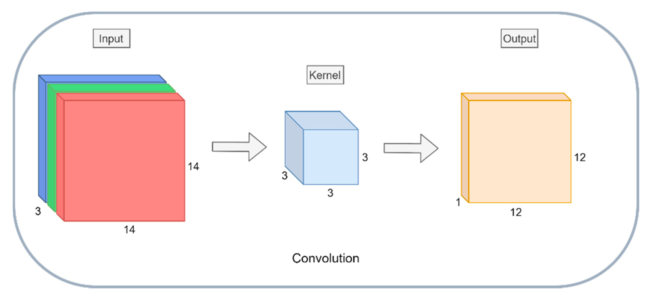
2.1. Convolutional Neural Networks

Nowadays, with the implementations of frameworks that allow us to make out own DL models for any specific task [16], it is not hard to develop a full-custom CNN from the beginning. On the contrary, there is no trivial way to get a custom model to perform well on the available data without often having to try tens of times and repeat several experiments. On the other hand, CV tasks have been greatly improved thanks to one of the most important challenges in history, the ImageNet Large Scale Visual Recognition Challenge (ILSVRC) [17] allowing us to develop deeper models of CNNs through techniques such as TL.

Before 2012, the ILSVRC challenge had been dominated by ML techniques that required to manually select the features in order to use for example a Support Vector Machine (SVM). However, in 2012, Krizhevsky, Sutskever, and Hinton [18] surpassed with a big margin the top-2 result, using a CNN in the ILSVRC 2012. Since then, and with the publication of the Deep Learning article [19], baseline models of CNN designed for CV tasks and normally trained in the ILSVRC, have been released to reuse the models. Examples of baseline models are VGG-16 network [13], Inception-v3 network [20], Residual Networks versions 1 and 2 (ResNet) [14,21], depth-wise separable convolutions networks (Xception) [22], Densely Connected Networks (DenseNet) [15], among others. These CNN baseline models are often used to implement new systems for CV task and for CADe and CADx [23].

2.2. Transfer Learning and Chest Diseases

Training a deep CNN model such as ResNet, Xception, or DenseNet from scratch requires a lot of data because they contain millions of trainable parameters, in which a small dataset would be insufficient to get a good generalization of the model. On the contrary, the mentioned baseline models have been used to compete in the ILSVRC through the years. Moreover, these models can be reused using their pre-trained weights employing a TL technique.

TL has been a useful ML method in which a pre-trained model of CNN is reused to take advantage of its weights to take them into account as initialization for a new CNN model for a different purpose [24]. There exist two primary ways to use TL from a model: reuse a model as a feature extractor and use a new totally different classifier; or reuse the model to perform Fine-Tuning (FT). FT is a technique that uses some unfrozen layers of a full model to slightly adjust both the new Fully Connected (FC) layers of the classifier and specific layers of the CNN like convolutional layers [25].

CNN applications for chest diseases began to popularize after Wang et al. [26] released the Chest-Xray14 dataset (CX14) in 2017, containing 108,948 posterior-anterior (PA) CXRAYs. Since then, multiple approaches of CNN for classification and segmentation tasks have been presented. One of the first was presented by Rajpurkar et al. [27], in which a pre-trained DenseNet called CheXNet was used in the CX14 dataset to classify the 14 diseases but used a new test set of CXRAY of pneumonia, achieving a radiologist-level diagnosis compared with board-members doctors from the Stanford University.

Blumenfeld, Greenspan, and Konen presented a CNN for Pneumothorax detection using CXRAY images [28].

Que et al. presented an automated method for cardiomegaly detection using two different architectures, one for segmentation, then a new one for classification [29].

Apart from CX14 dataset, in 2019 Irvin et al. published a new large dataset of CXRAY images, the CheXpert dataset [30], in which they provided 224,316 CXRAYs. They established a baseline result for the classification task of 14 different classes.

Allaouzi and Ahmed, presented a novel CNN [31] that achieved better performance in both, CX14 and CheXpert datasets, surpassing the baseline established by Irving et al.

Therefore, due to the popularity of CX14 dataset, we can find several works that use CX14 dataset and present novel results almost every two or three months, examples of these works are found in [32,33,34,35].

Works that have used the CX14 or CheXpert datasets commonly train from scratch a specific model of CNN due to the high availability of data, more than 100,000 images.

On the other hand, there exist some relevant datasets focused on chest diseases that are not big enough to train such big networks. For example, Kermany et al. [36], presented the Pneumonia dataset that only contains 5232 CXRAYs.

For Kermany’s dataset, there exist several classification works, like the one presented by Stephen et al. [34]. One of the most recent top results was by Liang and Zheng using an individual CNN model [37] and the most recent work by Chouhan et al. [38], that used an ensemble model. We will refer to Lian and Zheng network as LZNet2019 and to Chouhan et al. ensemble as Cho2020 for further comparisons.

In both works, they used a TL technique to reuse a pre-trained baseline model of CNN to classify and visualize the CXRAYs with pneumonia.

Moreover, there exists efficient full-custom CNN as presented by Pasa et al. [39]. In this work, the proposed CNN is compared with some of the state-of-the-art methods that use TL techniques [40,41,42] to obtain better results.

Our proposal uses a TL method in conjunction with the Xception network as pre-trained model on ImageNet. This is due to the Xception model allows to develop CV applications without having datasets of tens of thousands of images available which is the common scenario in developing countries. We also use some preprocessing techniques performed to the CXRAYs in order to increase the performance of our method. Therefore, we aim to present an automatic tool to classify between chest diseases such as pneumonia and healthy patients to assist a medical diagnosis even when there are not available expert radiologists. Moreover, we compared our approach with other baseline models of CNN and recently published works to have a reference point of our results.

3. Materials and Methods

In this section, in the first place, we will introduce the dataset used for this research. An imbalance problem will be described, as well as the Convolutional Neural Network model used for the classification task. In addition, some performance measures will be explained.

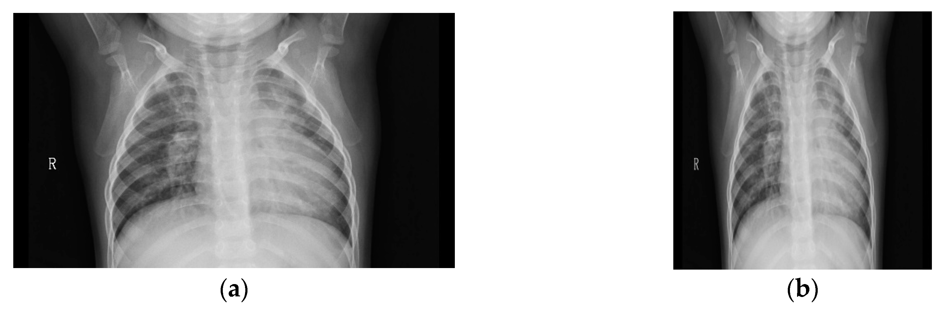
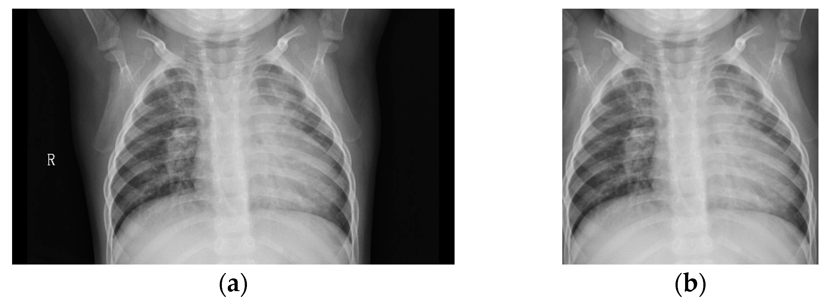
3.1. Pneumonia Dataset

The dataset used in this work was presented by Kermany et al. in 2018 [36]. It contains 5232 chest X-ray images from children from one to five years old. This dataset includes 3883 images characterized as depicting pneumonia (2538 bacterial, and 1345 viral) and 1349 labeled as normal images from a total of 5856 patients. The dataset includes its own test set with 234 normal images and 390 pneumonia images (242 bacterial and 148 viral) from the left 624 patients. Figure 1 shows an example of a CXRAY image labeled as normal and one with pneumonia.

The dataset [43] is available to download at: https://data.mendeley.com/datasets/rscbjbr9sj/2, under a Creative Commons Attribution 4.0 International licence. We use the version 2 of the dataset.

3.2. Class Imbalance

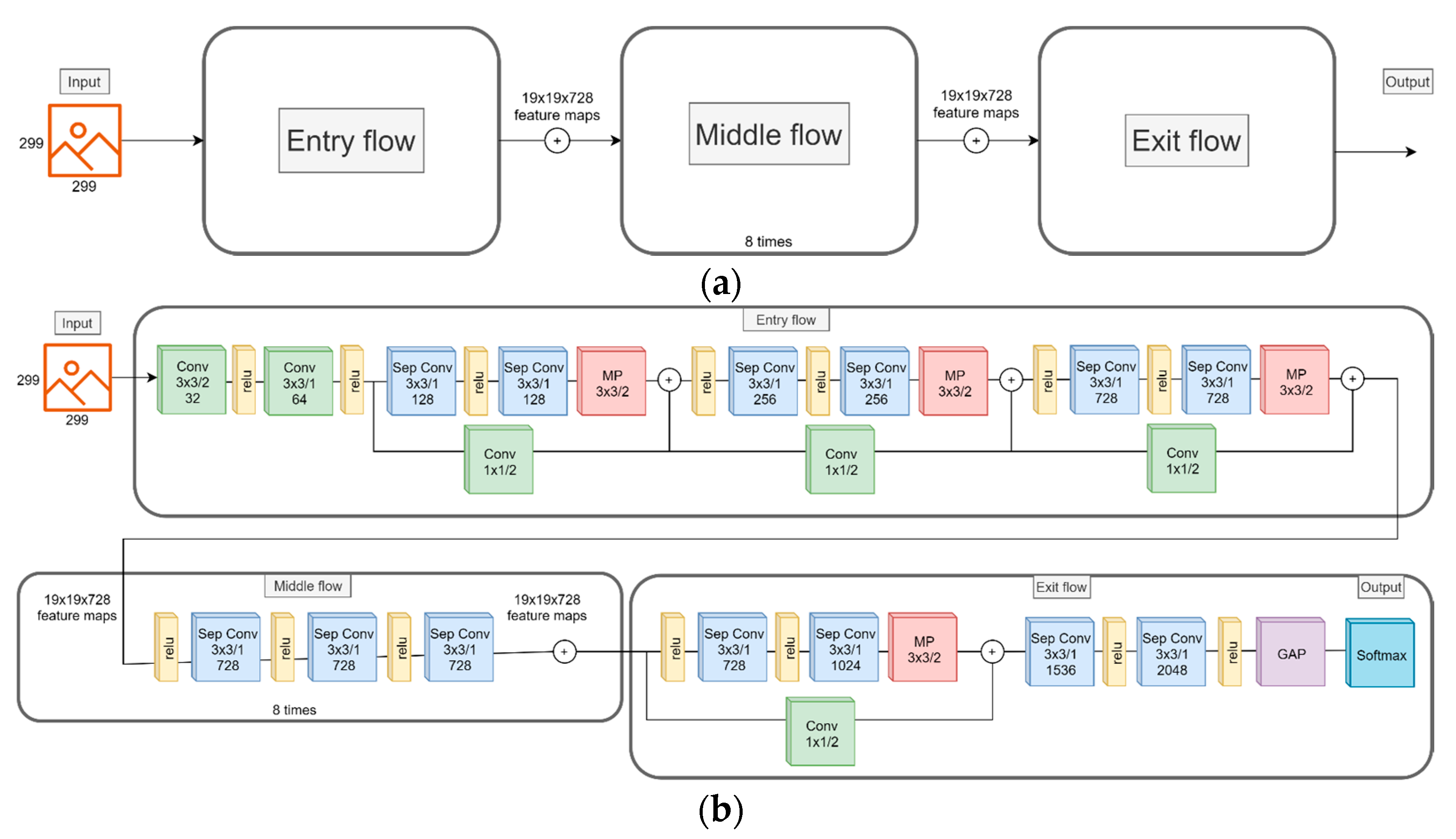
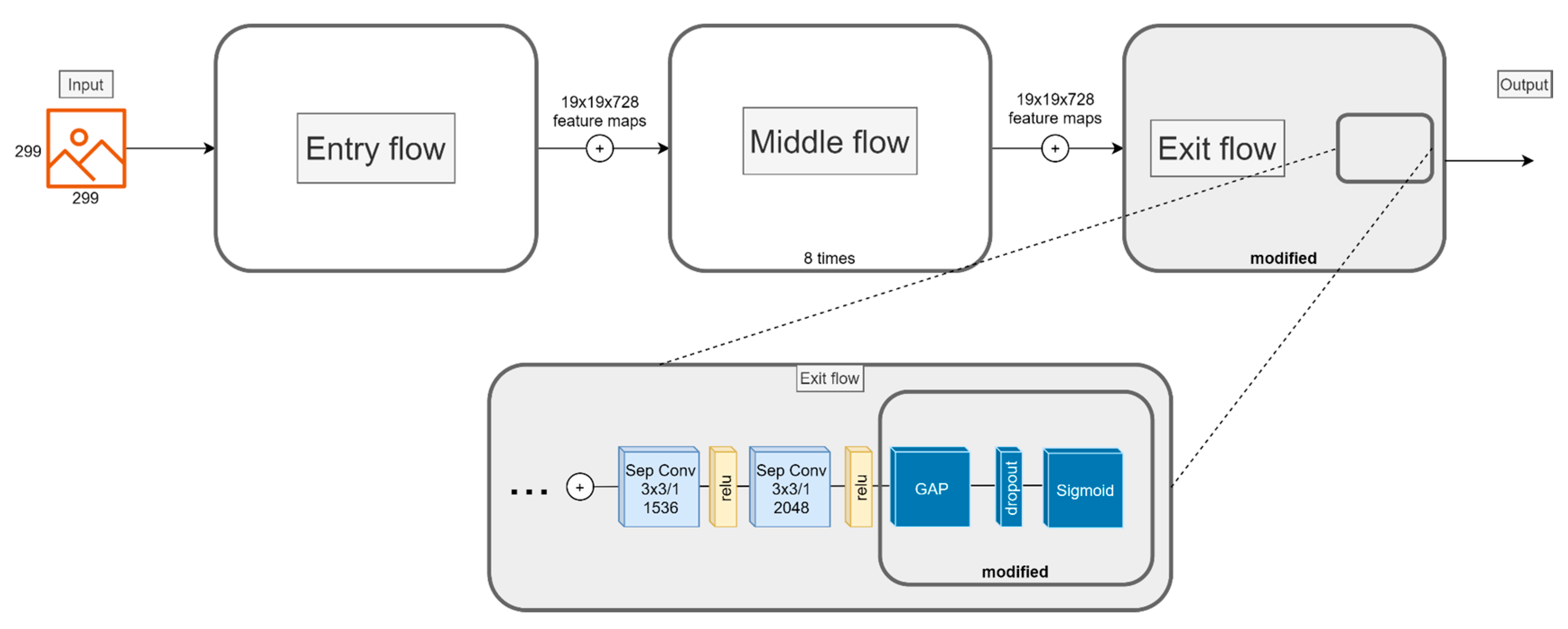
We can establish two different classes for this data set, NORMAL and PNEUMONIA. We can see that the two classes have different numbers of examples. We can compute the imbalance ratio (IR) of the training set as follows:

$$IR=\frac{\left|majority class\right|}{\left|minority class\right|}.$$

(1)

If $IR>1.5$ then, the dataset is imbalanced. Then IR of the pneumonia training set is:

$$IR=\frac{\left|PNEUMONIA\right|}{\left|NORMAL\right|}=\frac{3883}{1349}=2.87.$$

(2)

Then, $2.87>1.5$. Therefore, the pneumonia training set is imbalanced.

Class imbalance represents an important problem for intelligent classification algorithms. Moreover, standard evaluation metrics like accuracy do not offer a good measure of the performance of the algorithm. Therefore, it is important to select other metrics to try to address the imbalance problem [44].

The technique to address the imbalance problem will be covered in more detail in Section 4.2. On the other hand, metrics to evaluate the classification task will be detailed in Section 5.1.

3.3. CNN Model

We will explain some of the important details of the CNN model used in this research. The Xception model was created by François Chollet in 2016 [22]. The Xception architecture outperformed the VGG-16, ResNet50, ResNet101, ResNet152, and Inception-V3 on ImageNet [22].

The Xception model has its foundations in previous models like the original Inception [45] and the Inception-V3 [20]. Following the same basic structure, the Xception network has its main differences on the use of Depthwise Separable Convolutions (DWSC) instead of traditional Convolutions, and Residual Connections (RC) similarly to the introduced on the ResNet models. The architecture is constructed by 36 convolutional layers forming the feature extraction base. The 36 convolutional layers are structured into 14 modules in which only the first and last one do not contain residual connections.

The Depthwise convolution is “a spatial convolution that performs independently over each channel of an input, followed by a pointwise convolution, i.e., a 1 × 1 convolution, projecting the channel’s output by the Depthwise convolution onto a new channel space” [22]. Figure 2 shows an example of a traditional convolution. On the other hand, an example of DWSC is shown in Figure 3.

First, the final output of both traditional convolution and DWSC is the same, but as we can observe, the process performed by using a DWSC seems more complicated and extensive. In practice, the DWSC performs fewer operations, decreasing the computational cost of the network. With DWSC we can get deeper models that are more efficient than wider ones. On the other hand, even though the Xception model has a lot of parameters (more than 20 million) is more efficient and faster than the VGG-16 model.

Xception modules are different than the ones found in the Inception models because of the integration of DWSC. Figure 4 shows the general structure of the Xception model. When this model was used for classification on ImageNet, the final output layer consisted of 1000 neurons with activation function Softmax in order to predict a probability for the 1000 classes [22].

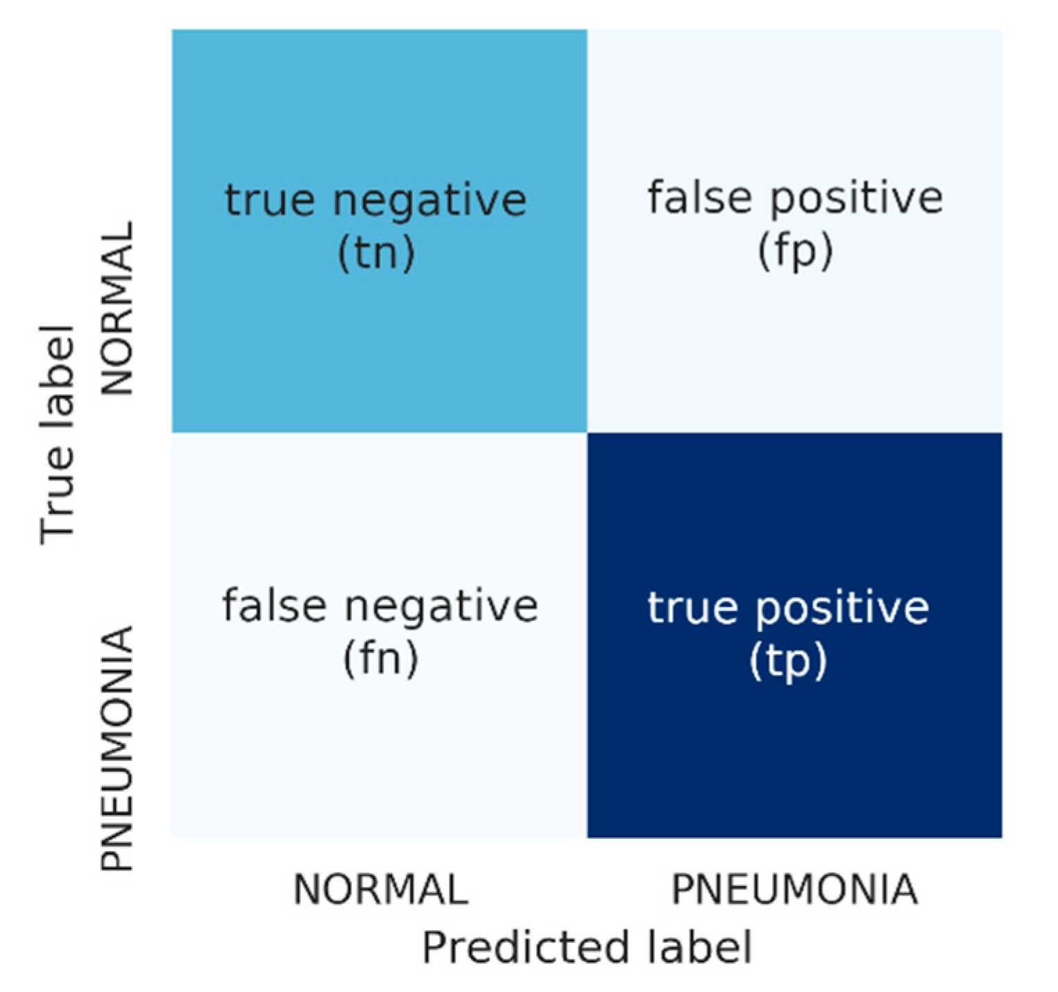
3.4. Performance Measures

In a classification task, the results can be expressed in an especial matrix called Confusion Matrix (CM). In a binary classification task, a CM contains the following information: class of the instances, and the number of instances classified as true positives (tp) that are the ones correctly recognized of the class of interest; true negatives (tn) that are the number of instances correctly recognized that belong to the other class; false positives (fp) are instances that were assigned to the class of interest but do not belong to it; and false negatives (fn) that represent instances that were assigned to the class of interest but belong to the complementary or negative class [46]. Figure 5 represents the convention of CM used in this research.

A common method to evaluate the performance of a classification model is to use specific metrics measures based on the values contained in a CM. Accuracy is the most common measure used for binary classification and evaluates the overall effectiveness of a classifier. Accuracy is defined as follows:

$$Accuracy=\frac{tp+tn}{tp+fn+fp+tn}.$$

(3)

However, when working with an imbalanced dataset is common to use different performance measures in addition to the Accuracy. The most common are precision, recall (formally named sensibility), and the F1-Score. A graphic such as the reception operating characteristic curve (ROC curve) and the measure associated with it, the area under the curve (AUC) is also useful. These measures are defined below.

$$Precision=\frac{tp}{tp+fp}$$

(4)

$$Recall=\frac{tp}{tp+fn}$$

(5)

$$F1-Score=\frac{2 tp}{2 tp+fp+tn}=2\frac{precision\times recall}{precision+recall}.$$

(6)

4. Proposal

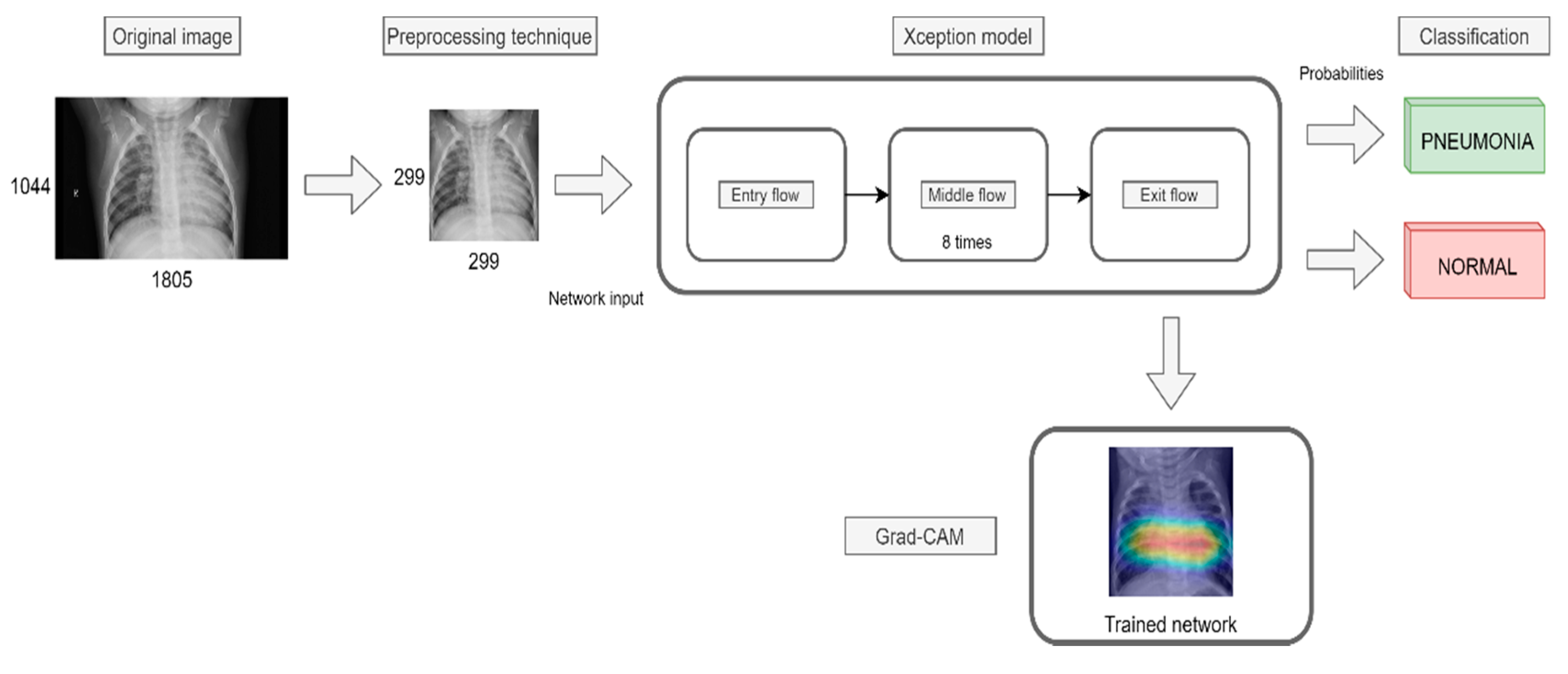
4.1. Image Preprocessing

Pretrained models use always squared images as input. CXRAY images from Pneumonia dataset are not squared, the biggest image has dimensions of 2916 × 2583 pixels, and the smallest is 384 × 127 pixels. If we only resized the images to match the input dimension for the CNN, we would have enlarged images that could probably suppress the features of interest. Figure 6 shows an example of a resized image compared with the original.

We use a simple preprocessing technique, proposed by Pasa et al. [39] to maintain as much information as possible of the region of interest of the CXRAY images.

Steps are as follows:

• Remove any possible black band from the edges of the image.
• Resize the image to achieve that the smaller edge is (in our case) 299 pixels long.
• Extract the central 299 × 299 region.

An example of the preprocessing technique is shown in Figure 7.

With this preprocessing technique, we are trying to use all the information on the image and feed the network with only pixels that are of interest and avoiding black spaces that do not provide any information to extract useful features for the classification task.

The media value of the training set was computed and subtracted from the training, validation and test sets, and all three were divided by the standard deviation of the training set. In other words, the distribution of the dataset was established with media $\mu =0$ and standard deviation $\sigma =1$. This process is known as Standardization.

4.2. Undersampling

As mentioned in Section 3.2, class imbalance represents an important problem to the classification task. Moreover, in neural networks and binary classification, this affects the behavior in training time because the cost function will be biased by the majority class.

One simple mechanism to attack this problem in the Pneumonia dataset is to balance the training set. In this work, we propose to use Random Undersampling (RUS).

Batista, Prati, and Monard [47] define the Random Undersampling as a non-heuristic method to help to combat the imbalance problem. It consists of the random elimination of samples of the majority class to obtain a balanced dataset.

For the Pneumonia dataset, RUS was performed in order to balance the training and validation sets. Therefore, 2534 CXRAY images were eliminated from the PNEUMONIA class, obtaining an equal NORMAL and PNEUMONIA instances of each class. Consequently, the final dataset used for this work contains a total of 2698 CXRAY images for the training and the validation sets.

4.3. Cost-Sensitive Learning

Cost-Sensitive Learning (CSL) consists of applying a specific penalty to examples of each class when evaluating the cost function in the classification task [48]. Cost function penalties can be specified as a matrix of weights to establish some priority to specific classes. In this work, despite the training and validation sets had been balanced by RUS, CSL was applied to correct the biased results from the CNN.

Table 1. Matrix of penalties applied to the cost function in order to avoid biased results from the CNN.

Class	Weight
NORMAL	5.0
PNEUMONIA	0.5

shows the weights used to penalize the cost function in the Xception network.

4.4. Transfer Learning

Pretrained weights on ImageNet were used as the TL method not to perform FT with some unfrozen layers, but as initialization in order to train end-to-end the network with the Pneumonia dataset. We use the Xception model with the weights of ImageNet and the following modifications were made to the original model: two last layers (logistic and pooling) were removed from the original model, and a new Global Average Pooling layer (GAP) was inserted, followed by a dropout layer with 0.25 of keeping rate. Finally, a logistic layer of two neurons with Sigmoid activation was collocated at the end of the network to predict the probability of the classes. Figure 8 shows a diagram of the section modified within the network.

The introduced modifications allow our model to have a new initialized decision layers to adapt the pre-trained model to the new one.

4.5. Data Augmentation and Hyperparameter Tuning

Data augmentation was performed as a regularization mechanism to avoid immediate overfitting. Operations performed at real-time over the training set are as follow:

• Horizontal flipping
• Zoom range of ±10%
• Random rotation of ±0.1 degrees.

After several experiments, we found that almost no rotation gave better results. Even though random rotation is almost inexistent, the samples with these operations are not the same as the ones that are not rotated. We tried other data augmentation techniques such as horizontal and vertical shift with ±10%, and a change of brightness of ±10% without finding any improvement.

Moreover, apart from preprocessing the images, hyperparameters represented a vital part of the training. The best model for the classification of the Pneumonia dataset was obtained after multiple configurations. The hyperparameters of the final model used for this work are shown in

Table 2. Network hyperparameters.

Cost Function	Learning Rate (Lr)	Optimizer	No. Epochs	Batch Size	Lr Decay
Binary cross entropy	$1\times {10}^{-3}$	Adam ${\beta }_1=0.9$ ${\beta }_2=0.999$	100	32	10 times after a plateau

.

As indicated in Table 2, the optimization target function also known as cost function or loss, used in this CNN was Binary Cross-Entropy, which is defined as follows:

$$H\left(p,q\right)=-{\displaystyle \sum }_i{p}_i\log {\mathrm{q}}_{\mathrm{i}}=-y\log \widehat{y}-\left(1-y\right)\log \left(1-\widehat{y}\right).$$

(7)

If we apply the weights matrix of CSL, we will have:

$$H\left(p,q\right)=-5y\log \widehat{y}-0.5\left(1-y\right)\log \left(1-\widehat{y}\right).$$

(8)

As shown in Equation (4), we used CSL in order to avoid the bias prediction of the network when training the model. In other words, we optimize the cost function giving preference to the NORMAL class instead of PNEUMONIA because of the nature of the dataset, in which healthy patients are minority.

5. Results

In this section, the conducted experiments will be explained. Implementation details will be mentioned. We include the explanations for the experimental framework used, as well as the validation and test results obtained.

5.1. Experimental Framework

After applying the proposed preprocessing technique and solve the problem of imbalanced sets we used a total of 2698 CXRAY images. Upon the final images, a partition was performed with an 80-20 hold-out as a validation method. It is important to note that the partition used to obtain both training and validation sets were performed only once. Therefore, conducted experiments used always the same sets and a fixed seed was established in order to replicate the results. Finally, the test set was not modified by RUS, conserving all 624 instances for testing purposes.

The Xception CNN model used in this research, and the models used for comparison were implemented in the Deep Learning framework Keras [16] that includes the tool for data augmentation. The pre-processing technique and RUS were both implemented in Python 3.6 using OpenCV [49] as the main image processor library. All experiments were conducted in the Google Collaboratory platform that in our experiments provides a Linux platform with 12 GB of RAM and a GPU Nvidia Tesla K80 with 12 GDDR VRAM. The average training time was 53 s per epoch, 0.779 s per batch. Therefore, each example was processed in approximately 0.0244 s.

Experimental framework and proposed methodology summaries as follow:

• RUS is performed over the original training data of the Pneumonia dataset.
• Hold-out 80-20 was performed in order to obtain the training and validation sets.
• Pre-processing technique was applied to training, validation and original test sets.
• Training and validation sets were fed into the network.
• The test set was fed into the trained network to obtain the classification results.
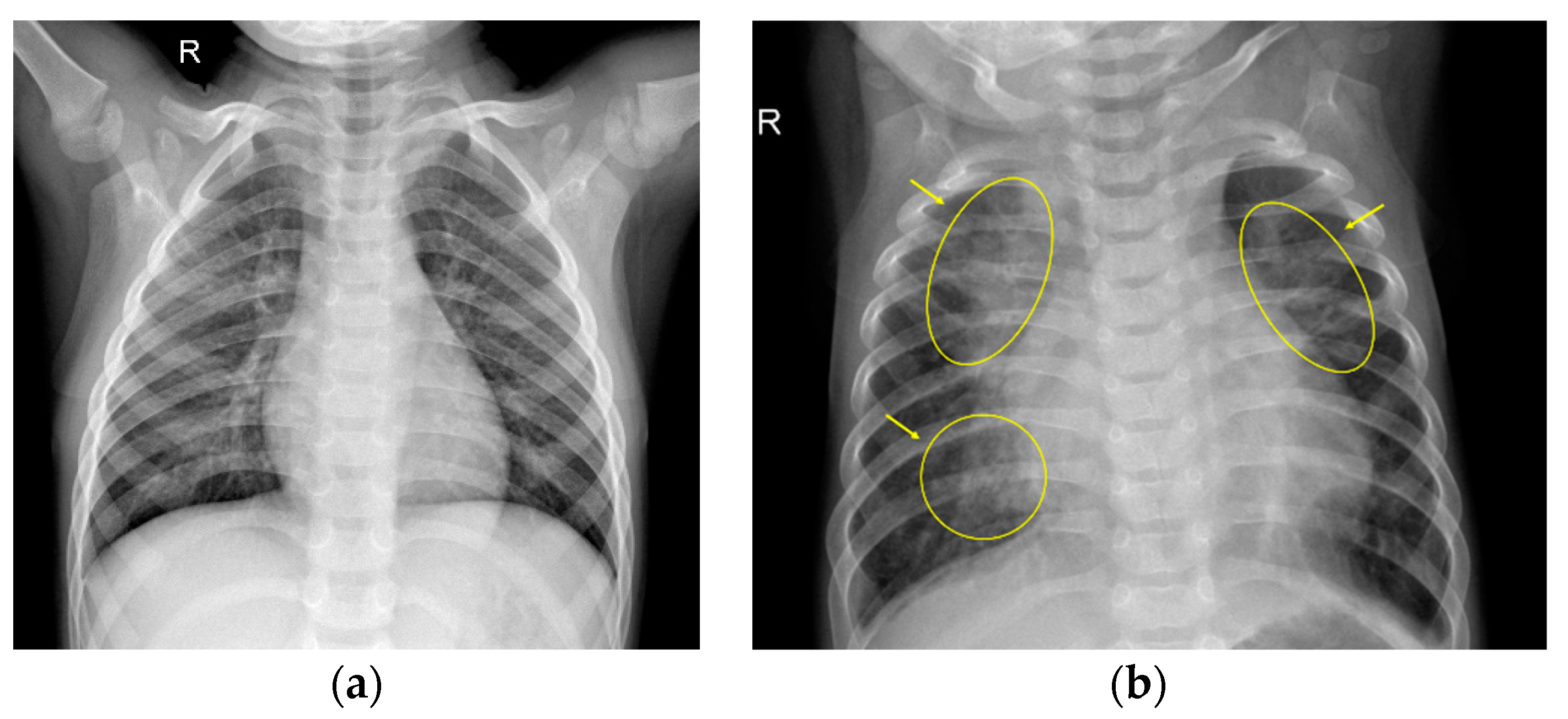
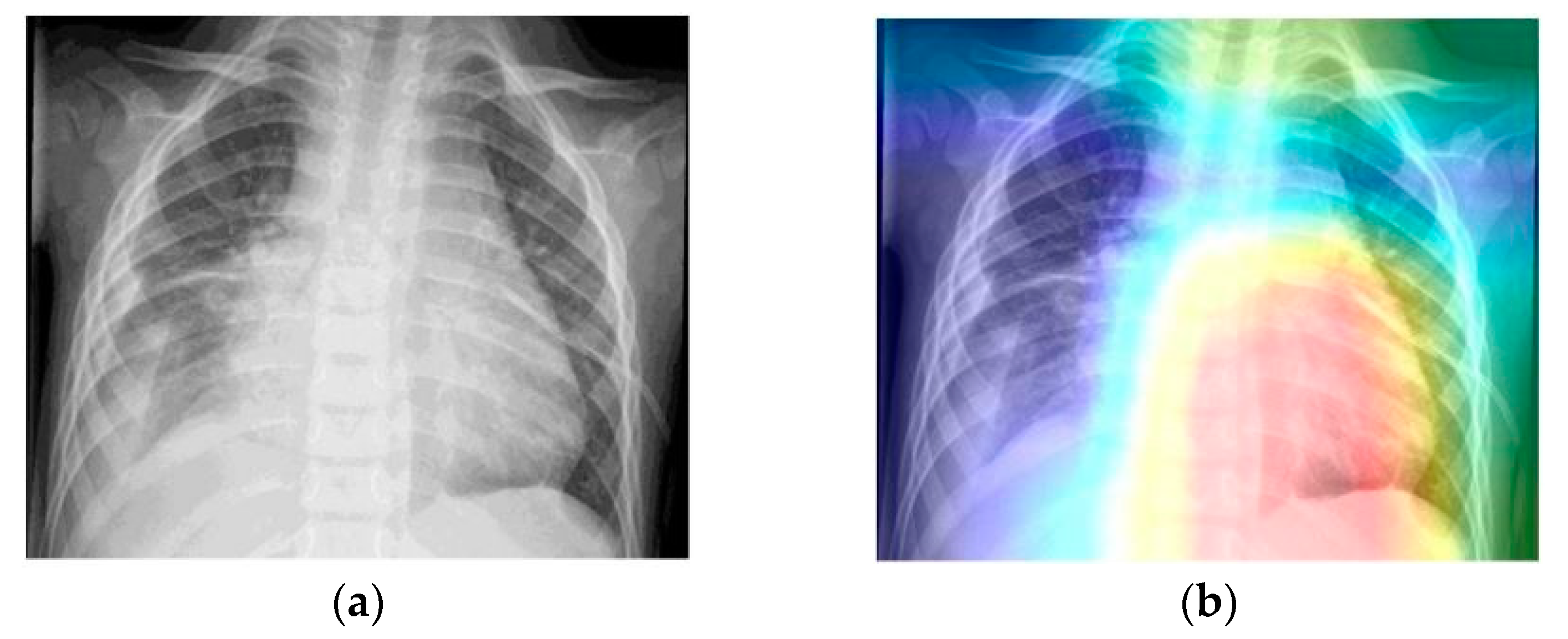
• Grad-CAM was used in order to generate a heatmap of the possible localization of pneumonia manifestations on test images.

Figure 9 shows the general diagram of the proposed methodology.

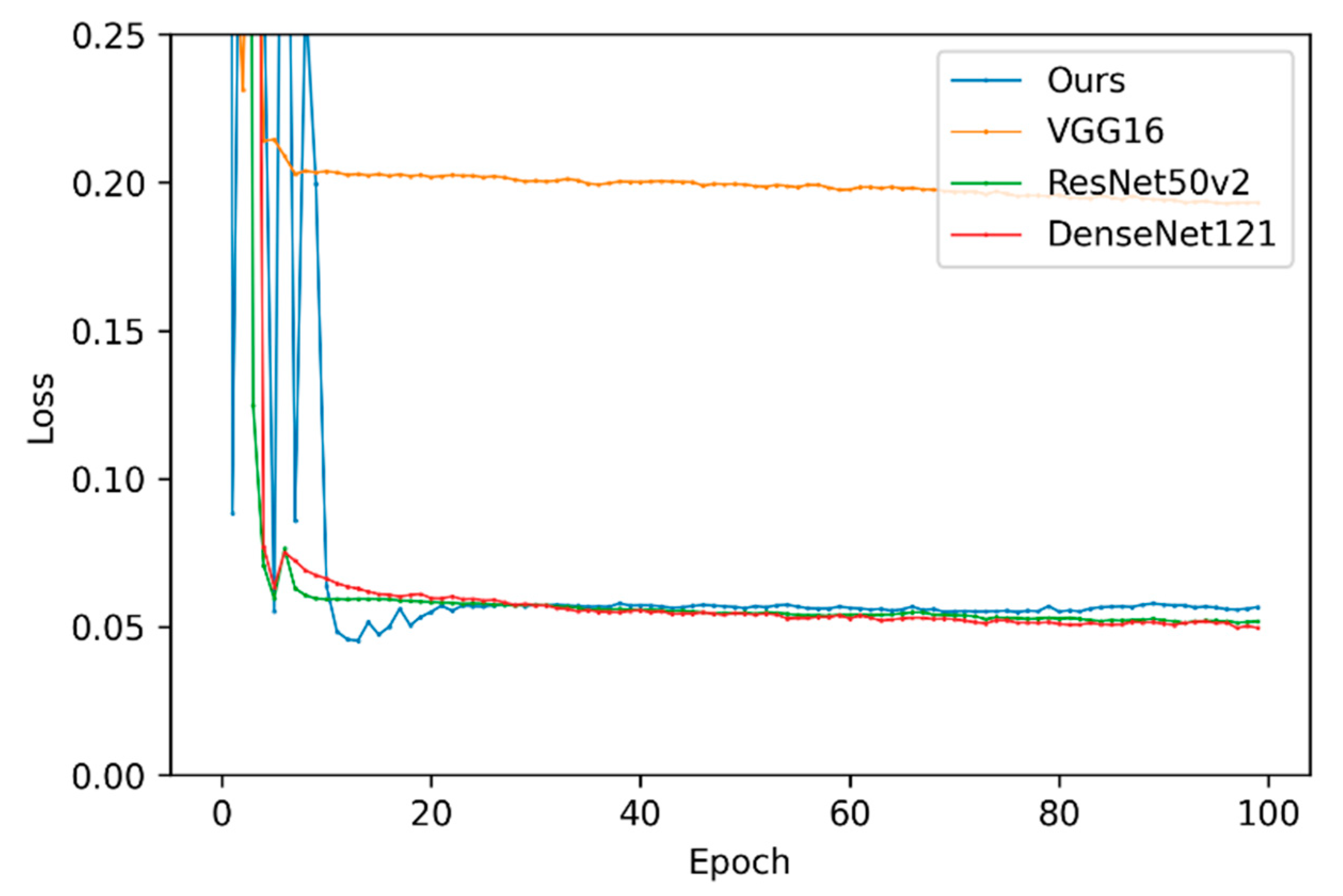
5.2. Validation Results

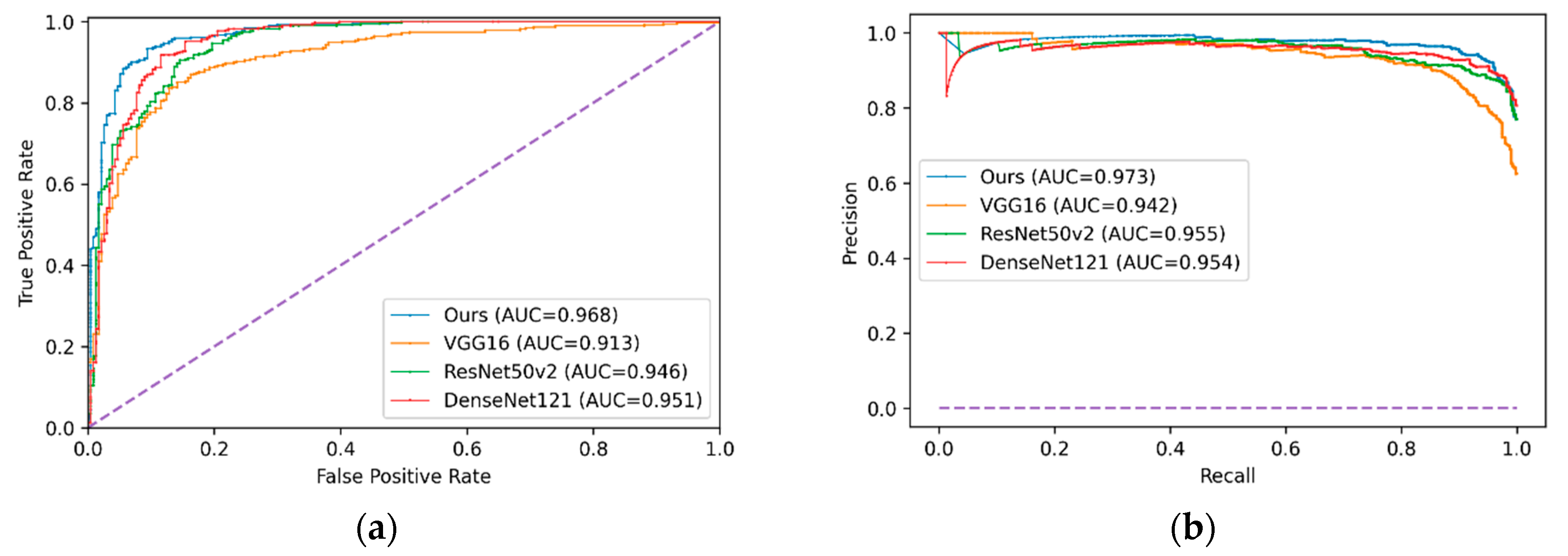
We performed some experiments training the proposed method and the baseline models on the training set, and then, we validate the model employing the validation set. Figure 10 shows the validation loss of both the proposed model and the state-of-the-art baseline models.

Measures of convergence and training time for the proposed model and the baseline models are condensed in

Table 3. Comparison of validation loss and training time for all models.

Model	Best Epoch	Validation Loss	Average Training Time (Epoch)	Average Training Time (Example)	Convergence Time (Best Model)
VGG-16	97	0.1928	44 s	0.0202 s	4268 s
ResNet50-v2	93	0.0514	43 s	0.0198 s	3999 s
DenseNet121	98	0.0496	51 s	0.0234 s	4998 s
Our model	14	0.0453	53 s	0.0244 s	742 s

. Best results for each column are highlighted in bold.

As shown in Table 3, our model converged 6.7 times faster than the second-fasted model. It just used 12 min to process the entire dataset, and to execute transfer learning.

5.3. Test Results

As mentioned in Section 3.1, the Pneumonia dataset contains its own test set. After performing several experiments, we selected the model that performed best in the validation set taking into account the value of loss of the cost function, and then evaluate the full test set.

To highlight the advantages of the proposed model, we compared with some of the state-of-the-art baseline models used for CV task and medical images applications as VGG-16 [13], ResNet50v2 [14], DenseNet121 [15] and the LZNet2019 [37] that was the top result until the development of this research.VGG-16 and DenseNet121 use images of dimensions 224 × 224 as input. Moreover, the LZNet2019 uses 150 × 150 as input. On the other hand, our model uses 299 × 299 as the input shape. We need to mention that VGG-16, ResNet50v2, and DenseNet121 were fed with the same images as the proposed model. The CM and performance measures of classification results for all models are shown

Table 4. Confusion Matrices (CMs) and performance measures of different models for pneumonia classification on the test set. Green fields were found by reverse engineering of paper metrics.

Model	Confusion Matrix		Precision	Recall	F1-Score	ROC Curve AUC	Precision–Recall AUC
VGG-16	184	50	0.874	0.892	0.883	0.913	0.942
	42	348
ResNet50-v2	156	78	0.832	0.990	0.904	0.946	0.955
	4	386
DenseNet121	159	75	0.838	0.992	0.908	0.951	0.954
	3	387
LZNet2019	188	46	0.891	0.967	0.927	0.953	-
	13	377
Cho2020	207 *	31 *	0.932	0.996	0.959 *	0.993	-
	4 *	386 *
Our model	162	72	0.843	0.992	0.912	0.968	0.973
	3	387

* Numbers obtained by reverse engineer of the results offered in the corresponding paper.

. Best results for each measure are in bold.

In order to offer a more precise analysis of the proposed method compared with the baseline models, we show the ROC curves with its respective AUC, and the precision–recall curves with its own AUC in Figure 11.

6. Discussion

In this section, an analysis of the baseline CNN models compared with the proposed model will be established based on the results exposed in Section 4. We will argue about the advantages of our model for the classification of the Pneumonia dataset. In addition, we evaluate the performance of the model with Gradient-weighted Class Activation Mapping (Grad-CAM) [50], which offers a heat-map of the possible localization of pneumonia manifestations.

Grad-CAM is a technique used to produce “visual explanations” of CNN models using the gradient of a target concept. The target flows into the final convolutional layer to produce a coarse localization map highlighting the important regions in the image of the prediction concept. In this research, the radiopaque segments that are correctly detected by the filters, and represented in the feature maps of the Xception mode when classifying between NORMAL and PNEUMONIA are highlighted using the gradients of the last Convolutional layer inside the 14th convolutional block.

A brief explanation will be stated about the problems of Grad-CAM on the pneumonia images. In Figure 12, examples of both correctly and incorrectly classified images with their corresponding heat-map are displayed.

On the validation results at training time (Table 3), the proposed model outperformed all the baseline models. Our proposal achieved a validation loss of 0.0453 at epoch 14. On the contrary, VGG16 obtained a loss of 0.1928 at epoch 97; ResNet50v2 obtained a loss of 0.0514 at epoch 93; DenseNet121 obtained a loss of 0.0496 at epoch 98.

The training time of a DL algorithm is an important factor in order to select a specific model for a specific task. As mentioned in Section 5.1, our model took 53 s for the epoch. Time for baselines models were as follows: VGG took 44 s per epoch; ResNet50v2 took 43 s per epoch; DenseNet121 took 51 s epoch. As a result, our best model took 742 s to converge compared with 4998 s for the up-runner model. Therefore, our proposal can converge in a better solution compared with baseline models up to 5.4 to 6.7 times faster.

The performance measures obtained from the CM of the proposed model are condensed in Table 4. As we can observe, our model achieves a Precision of 0.845; this is not the top result but outperforms all the baseline models. This measure indicates the agreement of the correct classes with the correctly classified by our model. Recall is possible one of the most important measures for medical applications because it indicates the effectiveness of the model to identify the class of interest, that in this case are the instances of PNEUMONIA class. We reconstructed the CM for Cho2020 as a request of an anonymous reviewer, by reverse engineering of the results presented in their paper. We obtained a high recall of 0.992 similarly to DenseNet121, but outperformed it on all the left measures. The F1-Score, that is the harmonic mean between precision and recall illustrates the relation between positive instances of both classes and the ones predicted by the model. We obtained an F1-Score of 0.914, just under LZNet2019 and Cho2020, surpassing again all the baseline models. AUC represents the ability of the model to avoid false classification, we obtained an AUC value of 0.963 that is the best among all baseline models and LZNet2019.

Furthermore, we elaborated and showed the precision–recall curves that are recommended for skewed domains where sometimes the ROC curve provides an excessively optimistic performance. In precision–recall curves, we also compute their own AUC, obtaining a high value of 0.971 compared with all baseline models.

Then, the proposed model achieves to outperform the baseline models in all measures, and the LZNet2019 results in the two most important measures for both medical classification tasks and imbalanced problems such as Recall and AUC of ROC curve. It is worth mentioning that these scores were achieved with a Transfer Learning method from ImageNet that is from a totally different context and we use the weights of the pre-trained Xception model to initialize the proposed model. We also stand out that we did not have the need to train the model of this research in a similar big dataset as CX14, compared with the LZNet2019. This allowed us to train a full model with the Pneumonia dataset in a quick way, without previous CXRAY images.

Additionally, we provide a Grad-CAM to visualize the possible localization of the pus, fluid and condensations caused by the Pneumonia. Figure 13 shows examples of generated heat-maps and one from LZNet2019.

As we can observe, the proposed model correctly identifies manifestations of Pneumonia in CXRAY images as seen in (a) and (c) from Figure 12, in which they present radiopaque segments in the right lower area of the patients. On the contrary, (g) and (h) are a misclassified example from the NORMAL class. In addition, we also highlight two glitches in which the Xception model presented problems of localization. First, the model confuses the texture of the heart as Pneumonia manifestations. That is the reason why, in the heat-maps of Figure 12, an activation is detected on the left inferior segment of the patients, specifically in (d); and (b) from Figure 13 show that the infection is on the heart, but in reality, the radiopaque segments are located on the upper part of the lungs in both sides; the second problem was that with a lot of instances of the CXRAY images being of children, the thymus is commonly detected in the NORMAL examples, or in this case, as the upper activation in (b) from Figure 12. Finally, we took the Grad-CAM example of LZNet2019 from Figure 13 and detected that they presented the same problem as in (d) and (f) from Figure 12. Moreover, it seems that only the heart was detected. Then, neither consolidations nor radiopaque segments of pneumonia manifestations were correctly identified. Therefore, our proposal provides better results on localization.

7. Conclusions

In this paper, we present a transfer learning method that automatically classifies between chest X-ray images of people that do not have a pulmonary disease, labeled as NORMAL, and people that have Pneumonia disease, labeled as PNEUMONIA. The proposed method uses a Transfer Learning technique to use the Xception Convolutional Neural Network pre-trained weights on ImageNet as an initialization for the new model. This network has 36 convolutional layers, and for the output, flow contains a Global Average Pooling layer, a dropout of 0.25 keep rate, and a logistic layer of two neurons with Sigmoid as activation function. Images are preprocessed to eliminate black segments, weights are assigned to penalize the cost function, and Adam optimizer is used to minimize the binary cross-entropy function. With the transfer learning, we overcome the problem of having a huge dataset of images. Our method outperforms baseline models and state-of-the-art previous results work in some performance measures. Moreover, we achieve a precision score of 0.843; a recall score of 0.992; an F1-Score of 0.912; an AUC score of 0.962 for the ROC curve; and an AUC score of 0.973 for precision–recall curves. In addition, our proposal is up to 5.4 to 6.7 times faster compared with the baseline models used in this research.

As future work, we would want to consider invariance of results on image shifts, and both preprocessing and data augmentation techniques that involve brightness and contrast changes, as well as image warping. In addition, we would also try using an automatic parameter-tuning method and apply the proposed algorithm to several medical image dataset, in order to make a statistical analysis of its performance.

References

1. Mahomed, N.; van Ginneken, B.; Philipsen, R.H.; Melendez, J.; Moore, D.P.; Moodley, H.; Sewchuran, T.; Mathew, D.; Madhi, S.A. Computer-aided diagnosis for World Health Organization-defined chest radiograph primary-endpoint pneumonia in children. Pediatr. Radiol. 2020, 50, 482–491. [Google Scholar] [CrossRef]
2. Doi, K. Computer-Aided Diagnosis in Medical Imaging: Historical review, current status and future potential. Comput. Med. Imaging Graph. 2007, 31, 198–211. [Google Scholar] [CrossRef] [PubMed] [Green Version]
3. Suetens, P. Fundamentals of Medical Imaging, 2nd ed.; Cambridge University Press: New York, NY, USA, 2009; pp. 14–32. [Google Scholar]
4. Aliyu, G.; El-Kamary, S.S.; Abimiku, A.L.; Hungerford, L.; Obasanya, J.; Blattner, W. Cost-effectiveness of point-of-care digital chest-x-ray in HIV patients with pulmonary mycobacterial infections in Nigeria. BMC Infect. Dis. 2014, 14, 675. [Google Scholar] [CrossRef] [PubMed] [Green Version]
5. Sutton, D. Textbook of Radiology and Imaging, 7th ed.; Churchill Livingstone Elsevier: London, UK, 2003; pp. 131–135. [Google Scholar]
6. Anwar, S.M.; Majid, M.; Qayyum, A.; Awais, M.; Alnowami, M.; Khan, M.K. Medical Image Analysis using Convolutional Neural Networks: A Review. J. Med. Syst. 2018, 42, 226. [Google Scholar] [CrossRef] [PubMed] [Green Version]
7. Talo, M.; Baloglu, U.B.; Yıldırım, Ö.; Rajendra Acharya, U. Application of deep transfer learning for automated brain abnormality classification using MR images. Cogn. Syst. Res. 2019, 54, 176–188. [Google Scholar] [CrossRef]
8. Li, Z.; Wang, C.; Han, M.; Xue, Y.; Wei, W.; Li, L.J.; Fei-Fei, L. Thoracic Disease Identification and Localization with Limited Supervision. In Deep Learning and Convolutional Neural Networks for Medical Imaging and Clinical Informatics. Advances in Computer Vision and Pattern Recognition; Springer: Cham, Swizterland, 2019; pp. 139–161. [Google Scholar]
9. Fang, W.; Zhong, B.; Zhao, N.; Love, P.E.; Luo, H.; Xue, J.; Xu, S. A deep learning-based approach for mitigating falls from height with computer vision: Convolutional neural network. Adv. Eng. Inform. 2019, 39, 170–177. [Google Scholar] [CrossRef]
10. Wang, G.; Li, W.; Zuluaga, M.A.; Pratt, R.; Patel, P.A.; Aertsen, M.; Doel, T.; David, A.L.; Deprest, J.; Ourselin, S.; et al. Interactive Medical Image Segmentation Using Deep Learning With Image-Specific Fine Tuning. IEEE Trans. Med. Imaging 2018, 37, 1562–1573. [Google Scholar] [CrossRef]
11. Li, H.; Li, A.; Wang, M. A novel end-to-end brain tumor segmentation method using improved fully convolutional networks. Comput. Biol. Med. 2019, 108, 150–160. [Google Scholar] [CrossRef]
12. Chen, S.; Ding, C.; Liu, M. Dual-force convolutional neural networks for accurate brain tumor segmentation. Pattern Recognit. 2019, 88, 90–100. [Google Scholar] [CrossRef]
13. Geng, L.; Zhang, S.; Tong, J.; Xiao, Z. Lung segmentation method with dilated convolution based on VGG-16 network. Comput. Assist. Surg. 2019, 24, 27–33. [Google Scholar] [CrossRef] [Green Version]
14. Jung, M.; Chi, S. Human activity classification based on sound recognition and residual convolutional neural network. Autom. Constr. 2020, 114, 103177. [Google Scholar] [CrossRef]
15. Yao, Z.; Li, J.; Guan, Z.; Ye, Y.; Chen, Y. Liver disease screening based on densely connected deep neural networks. Neural Netw. 2020, 123, 299–304. [Google Scholar] [CrossRef] [PubMed]
16. Chollet, F. Keras: The Python Deep Learning library. Available online: https://keras.io/ (accessed on 2 November 2019).
17. Russakovsky, O.; Deng, J.; Su, H.; Krause, J.; Satheesh, S.; Ma, S.; Huang, Z.; Karpathy, A.; Khosla, A.; Bernstein, M.; et al. ImageNet Large Scale Visual Recognition Challenge. Int. J. Comput. Vis. 2015, 115, 211–252. [Google Scholar] [CrossRef] [Green Version]
18. Krizhevsky, A.; Sutskever, I.; Hinton, G.E. ImageNet Classification with Deep Convolutional Neural Networks. In Proceedings of the Advances in Neural Information Processing Systems (NIPS’12), Lake Tahoe, NV, USA, 3–6 December 2012. [Google Scholar]
19. LeCun, Y.; Bengio, Y.; Hinton, G. Deep learning. Nature 2015, 521, 436–444. [Google Scholar] [CrossRef]
20. Szegedy, C.; Vanhoucke, V.; Ioffe, S.; Shlens, J.; Wojna, Z. Rethinking the Inception Architecture for Computer Vision. In Proceedings of the 29th IEEE Conference on Computer Vision and Pattern Recognition CVPR 2016, Las Vegas, NV, USA, 26 June–1 July 2016; IEEE: Danvers, MA, USA, 2016; pp. 2818–2826. [Google Scholar]
21. He, K.; Zhang, X.; Ren, S.; Sun, J. Deep Residual Learning for Image Recognition. In Proceedings of the 29th IEEE Conference on Computer Vision and Pattern Recognition CVPR 2016, Las Vegas, NV, USA, 26 June–1 July 2016; IEEE: Danvers, MA, USA, 2016; pp. 770–778. [Google Scholar]
22. Chollet, F. Xception: Deep Learning with Depthwise Separable Convolutions. In Proceedings of the 30th IEEE Conference on Computer Vision and Pattern Recognition CVPR 2017, Honolulu, HI, USA, 21–26 July 2017; IEEE: Danvers, MA, USA, 2017; pp. 1800–1807. [Google Scholar]
23. Bakator, M.; Radosav, D. Deep Learning and Medical Diagnosis: A Review of Literature. Multimodal Technol. Interact. 2018, 2, 47. [Google Scholar] [CrossRef] [Green Version]
24. Tsiakmaki, M.; Kostopoulos, G.; Kotsiantis, S.; Ragos, O. Transfer Learning from Deep Neural Networks for Predicting Student Performance. Appl. Sci. 2020, 10, 2145. [Google Scholar] [CrossRef] [Green Version]
25. Chollet, F. Deep Learning with Python, 1st ed.; Manning Publications Co.: Shelter Island, NY, USA, 2018; pp. 287–295. [Google Scholar]
26. Wang, X.; Peng, Y.; Lu, L.; Lu, Z.; Bagheri, M.; Summers, R.M. ChestX-Ray8: Hospital-Scale Chest X-Ray Database and Benchmarks on Weakly-Supervised Classification and Localization of Common Thorax Diseases. In Proceedings of the 30th IEEE Conference on Computer Vision and Pattern Recognition CVPR 2017, Honolulu, HI, USA, 21–26 July 2017; IEEE: Danvers, MA, USA, 2017; pp. 3462–3471. [Google Scholar]
27. Rajpurkar, P.; Irvin, J.; Ball, R.L.; Zhu, K.; Yang, B.; Mehta, H.; Duan, T.; Ding, D.; Bagul, A.; Langlotz, C.P.; et al. Deep learning for chest radiograph diagnosis: A retrospective comparison of the CheXNeXt algorithm to practicing radiologists. PLoS Med. 2018, 15, e1002686. [Google Scholar] [CrossRef]
28. Blumenfeld, A.; Greenspan, H.; Konen, E. Pneumothorax detection in chest radiographs using convolutional neural networks. In Proceedings of the Medical Imaging 2018: Computer-Aided Diagnosis, Houston, TX, USA, 27 February 2018. [Google Scholar]
29. Que, Q.; Tang, Z.; Wang, R.; Zeng, Z.; Wang, J.; Chua, M.; Gee, T.S.; Yang, X.; Veeravalli, B. CardioXNet: Automated Detection for Cardiomegaly Based on Deep Learning. In Proceedings of the 2018 40th Annual International Conference of the IEEE Engineering in Medicine and Biology Society (EMBC), Honolulu, HI, USA, 17–22 July 2018; IEEE: Danvers, MA, USA, 2018; pp. 612–615. [Google Scholar]
30. Irvin, J.; Rajpurkar, P.; Ko, M.; Yu, Y.; Ciurea-Ilcus, S.; Chute, C.; Marklund, H.; Haghgoo, B.; Ball, R.; Shpanskaya, K.; et al. CheXpert: A Large Chest Radiograph Dataset with Uncertainty Labels and Expert Comparison. In Proceedings of the AAAI Conference on Artificial Intelligence, Honolulu, HI, USA, January 27–1 February 2019; AAAI Press: Palo Alto, CA, USA, 2019; pp. 590–597. [Google Scholar]
31. Allaouzi, I.; Ben Ahmed, M. A Novel Approach for Multi-Label Chest X-Ray Classification of Common Thorax Diseases. IEEE Access 2019, 7, 64279–64288. [Google Scholar] [CrossRef]
32. Baltruschat, I.M.; Nickisch, H.; Grass, M.; Knopp, T.; Saalbach, A. Comparison of Deep Learning Approaches for Multi-Label Chest X-Ray Classification. Sci. Rep. 2019, 9, 6381. [Google Scholar] [CrossRef] [Green Version]
33. Chassagnon, G.; Vakalopolou, M.; Paragios, N.; Revel, M.P. Deep learning: Definition and perspectives for thoracic imaging. Eur. Radiol. 2020, 30, 2021–2030. [Google Scholar] [CrossRef]
34. Stephen, O.; Sain, M.; Maduh, U.J.; Jeong, D.-U. An Efficient Deep Learning Approach to Pneumonia Classification in Healthcare. J. Healthc. Eng. 2019, 2019, 1–7. [Google Scholar] [CrossRef] [PubMed] [Green Version]
35. Willemink, M.J.; Koszek, W.A.; Hardell, C.; Wu, J.; Fleischmann, D.; Harvey, H.; Folio, L.R.; Summers, R.M.; Rubin, D.L.; Lungren, M.P. Preparing medical imaging data for machine learning. Radiology 2020, 295, 4–15. [Google Scholar] [CrossRef] [PubMed]
36. Kermany, D.S.; Goldbaum, M.; Cai, W.; Valentim, C.C.S.; Liang, H.; Baxter, S.L.; McKeown, A.; Yang, G.; Wu, X.; Yan, F.; et al. Identifying Medical Diagnoses and Treatable Diseases by Image-Based Deep Learning. Cell 2018, 172, 1122–1131. [Google Scholar] [CrossRef]
37. Liang, G.; Zheng, L. A transfer learning method with deep residual network for pediatric pneumonia diagnosis. Comput. Methods Programs Biomed. 2019, 187, 104964. [Google Scholar] [CrossRef] [PubMed]
38. Chouhan, V.; Singh, S.K.; Khamparia, A.; Gupta, D.; Tiwari, P.; Moreira, C.; Damaševičius, R.; de Albuquerque, V.H.C. A novel transfer learning based approach for pneumonia detection in chest X-ray images. Appl. Sci. 2020, 10, 559. [Google Scholar] [CrossRef] [Green Version]
39. Pasa, F.; Golkov, V.; Pfeiffer, F.; Cremers, D.; Pfeiffer, D. Efficient Deep Network Architectures for Fast Chest X-Ray Tuberculosis Screening and Visualization. Sci. Rep. 2019, 9, 6268. [Google Scholar] [CrossRef] [Green Version]
40. Vajda, S.; Karargyris, A.; Jaeger, S.; Santosh, K.C.; Candemir, S.; Xue, Z.; Antani, S.; Thoma, G. Feature Selection for Automatic Tuberculosis Screening in Frontal Chest Radiographs. J. Med. Syst. 2018, 42, 146. [Google Scholar] [CrossRef]
41. Hwang, S.; Kim, H.-E.; Jeong, J.; Kim, H.-J. A novel approach for tuberculosis screening based on deep convolutional neural networks. In Proceedings of the Medical Imaging 2016: Computer-Aided Diagnosis, San Diego, CA, USA, 28 February–2 March 2016; Tourassi, G.D., Armato, S.G., III, Eds.; SPIE: Bellingham, WA, USA, 2016; pp. 750–757. [Google Scholar]
42. Chauhan, A.; Chauhan, D.; Rout, C. Role of gist and PHOG features in computer-aided diagnosis of tuberculosis without segmentation. PLoS ONE 2014, 9, e112980. [Google Scholar] [CrossRef]
43. Kermany, D.; Zhang, K.; Goldbaum, M. Labeled Optical Coherence Tomography (OCT) and Chest X-Ray Images for Classification. Available online: https://data.mendeley.com/datasets/rscbjbr9sj/2 (accessed on 7 October 2019).
44. López, V.; Fernández, A.; García, S.; Palade, V.; Herrera, F. An insight into classification with imbalanced data: Empirical results and current trends on using data intrinsic characteristics. Inf. Sci. (N.Y.). 2013, 250, 113–141. [Google Scholar] [CrossRef]
45. Szegedy, C.; Wei, L.; Yangqing, J.; Sermanet, P.; Reed, S.; Anguelov, D.; Erhan, D.; Vanhoucke, V.; Rabinovich, A. Going deeper with convolutions. In Proceedings of the 28th IEEE Conference on Computer Vision and Pattern Recognition CVPR 2015, Boston, MA, USA, 7–12 June 2015; IEEE: Danvers, MA, USA, 2015; pp. 1–9. [Google Scholar]
46. Sokolova, M.; Lapalme, G. A systematic analysis of performance measures for classification tasks. Inf. Process. Manag. 2009, 45, 427–437. [Google Scholar] [CrossRef]
47. Batista, G.E.A.P.A.; Prati, R.C.; Monard, M.C. A study of the behavior of several methods for balancing machine learning training data. ACM Sigkdd Explor. Newsl. 2004, 6, 20. [Google Scholar] [CrossRef]
48. López, V.; Fernández, A.; Moreno-Torres, J.G.; Herrera, F. Analysis of preprocessing vs. cost-sensitive learning for imbalanced classification. Open problems on intrinsic data characteristics. Expert Syst. Appl. 2012, 39, 6585–6608. [Google Scholar]
49. OpenCV. Available online: https://opencv.org/ (accessed on 2 November 2019).
50. Selvaraju, R.R.; Cogswell, M.; Das, A.; Vedantam, R.; Parikh, D.; Batra, D. Grad-CAM: Visual Explanations from Deep Networks via Gradient-based Localization. Int. J. Comput. Vis. 2020, 128, 336–359. [Google Scholar] [CrossRef] [Green Version]
Figure 1. Example of images that the pneumonia dataset contains in which (a) is a normal chest X-ray images (CXRAY) image with no radiopaque segments; (b) shows a CXRAY image from a patient with pneumonia, in which radiopaque segments with consolidations caused by fluid accumulation are visible. Original images are from (https://data.mendeley.com/datasets/rscbjbr9sj/2), a publicly available dataset. Manual annotations were performed by us with the assistance of a doctor.
Applsci 10 02908 g001
Figure 2. Example of operation of traditional convolution performed on an image as input of dimensions 14 × 14 × 3, with one kernel of dimension 3 × 3 × 3.
Applsci 10 02908 g002
Figure 3. Example of operation of Depthwise Separable Convolutions (DWSC) performed on an image as input of dimensions 14 × 14 × 3. First, a depthwise convolution is performed with three kernels of dimension 3 × 3 × 1, followed by a pointwise convolution with one kernel of 1 × 1 × 3.
Applsci 10 02908 g003
Figure 4. Xception model. (a) Shows the general structure of Xception model; (b) shows the detailed architecture of the original Xception model. After each convolution and separable convolution block, a batch normalization operation is performed. In a Conv block, for example, the first number indicates the size of the kernel, the second number indicates the size of the stride, and finally, the last number indicates the number of filters used in each specific block.
Applsci 10 02908 g004
Figure 5. Confusion matrix convention.
Applsci 10 02908 g005
Figure 6. Examples distortion on the images by applying only resizing to the dataset in order to adjust them to the input shape of the Convolutional Neural Networks (CNN) model. (a) shows the original image of a person with pneumonia (https://data.mendeley.com/datasets/rscbjbr9sj/2); (b) shows the resized image to 299 × 299 pixels.
Applsci 10 02908 g006
Figure 7. Preprocessing technique used in the Pneumonia dataset for all the examples. (a) The original image of a person with pneumonia (https://data.mendeley.com/datasets/rscbjbr9sj/2); (b) the preprocessed image with the final dimension of 299 × 299 pixels.
Applsci 10 02908 g007
Figure 8. Exit flow blocks modified in the proposed model.
Applsci 10 02908 g008
Figure 9. General workflow of the proposed methodology.
Applsci 10 02908 g009
Figure 10. Validation loss of all single CNN models.
Applsci 10 02908 g010
Figure 11. Metrics and curves of the implemented models where (a) shows the reception operating characteristic (ROC) curve and area under the curve (AUC); (b) shows the precision–recall curve with its respective area.
Applsci 10 02908 g011
Figure 12. Heat maps for classified test examples using Grad-CAM. (a,c,e,g) show a preprocessed CXRAYs; (b,d,f,g), show their respective Grad-CAM.
Applsci 10 02908 g012
Figure 13. An example of LZnet2019 performance. (a) is an original CXRAY and (b) its corresponding Grad-CAM from the LZNet2019 article.
Applsci 10 02908 g013