Optimising Hydrogel Release Profiles for Viro-Immunotherapy Using Oncolytic Adenovirus Expressing IL-12 and GM-CSF with Immature Dendritic Cells

Abstract

Sustained-release delivery systems, such as hydrogels, significantly improve cancer therapies by extending the treatment efficacy and avoiding excess wash-out. Combined virotherapy and immunotherapy (viro-immunotherapy) is naturally improved by these sustained-release systems, as it relies on the continual stimulation of the antitumour immune response. In this article, we consider a previously developed viro-immunotherapy treatment where oncolytic viruses that are genetically engineered to infect and lyse cancer cells are loaded onto hydrogels with immature dendritic cells (DCs). The time-dependent release of virus and immune cells results in a prolonged cancer cell killing from both the virus and activated immune cells. Although effective, a major challenge is optimising the release profile of the virus and immature DCs from the gel so as to obtain a minimum tumour size. Using a system of ordinary differential equations calibrated to experimental results, we undertake a novel numerical investigation of different gel-release profiles to determine the optimal release profile for this viro-immunotherapy. Using a data-calibrated mathematical model, we show that if the virus is released rapidly within the first few days and the DCs are released for two weeks, the tumour burden can be significantly decreased. We then find the true optimal gel-release kinetics using a genetic algorithm and suggest that complex profiles present unnecessary risk and that a simple linear-release model is optimal. In this work, insight is provided into a fundamental problem in the growing field of sustained-delivery systems using mathematical modelling and analysis.

1. Introduction

Controlled localised delivery systems have been replacing systemic administration of cancer therapies for some time [1]. These sustained-release injectable formulations are usually designed as microparticles, implants or gels [1]. They extend the presence of therapy at the tumour site by gradually releasing treatment as they degrade, improving treatment efficacy and avoiding excessive treatment loss to neighbouring tissue or the lymphatic system. Sustained-delivery systems have improved the effectiveness of a range of cancer treatments, including chemotherapy [2,3], oncolytic virotherapy [4,5,6,7] and immunotherapy [8,9,10].

Oncolytic virotherapy and immunotherapy are two promising cancer therapies that have gained significant attention over recent years [11]. Oncolytic virotherapy focuses on genetically engineering viruses to infect, replicate within, and lyse tumour cells. Many oncolytic viruses can accommodate gene insertions and thus be “armed” with therapeutic transgenes to produce immunostimulatory signals that stimulate an antitumour immune response, making them useful immunotherapy agents [12,13]. Immunotherapy treatments typically involve administration of additional cytokines, molecules or immature immune cells.

Interleukin 12 (IL-12) and granulocyte–monocyte colony-stimulating factor (GM-CSF) are cytokines used in immunotherapy clinical trials [14,15]. IL-12 is known to have potent antitumour effects through promotion of the immunity of helper T cells and activation of killer T cells, whereas GM-CSF is known to enhance the processing and presentation of antigen on antigen-presenting cells (APCs) [13]. Immature immune cells, such as dendritic cells (DCs), are also tested in immunotherapy trials with the goal of overcoming the induction of anergy or tolerance by the cancer [16,17]. Intratumoural administration of DCs increases the probability of tumour antigen recognition and subsequent activation of helper T cells and killer T cells, leading to heightened tumour cell killing [18].

An increasing number of studies has shown that combined virotherapy and immunotherapy (viro-immunotherapy) leads to a prolonged antitumour response, where both viruses and immune cells work simultaneously to eradicate cancer cells [10,13,19,20,21]. Conventionally, oncolytic virotherapy and immunotherapy are administered intratumourally or intravenously. This can result in rapid clearance of the virus and functional impairment of immune cells in the tumour microenvironment [10]. To overcome this, there have been many investigations into the potential of treatment loaded onto injectable gels or polymer matrix systems [5,6,7,10]. Oh et al. [10] showed that an oncolytic adenovirus expressing IL-12 and GM-CSF loaded onto a hydrogel with immature DCs had a higher retention in tumour tissue. Additionally, the use of the gel resulted in greater antitumour activity due to the sustained release of therapy. Immune checkpoint blockade therapy and agonists were also shown to be considerably more effective when loaded onto an degradable gel matrices [8,9]. A major challenge for sustained-release mechanisms is determining a release profile that achieves optimal therapeutic benefit.

Mathematical models describing the biological response to disease can be used as an important tool in therapy planning and optimisation [22,23,24,25]. Deterministic systems of ordinary differential equations (ODEs) are used to describe the key biophysical interactions and are then analysed to determine optimal therapeutic protocols [23]. In oncology, these techniques have been used to successfully optimise chemotherapy and immunotherapy treatment [25,26,27,28,29,30]. Zhu et al. [31] optimised the scheduling of one cycle of chemotherapy drug VP-16 and found a new optimal drug regime which improved the clinical efficacy. For combined immunotherapy and chemotherapy, de Pillis et al. [32] developed an ODE system that predicted which treatment protocols would result in tumour elimination. There are also a handful of examples where deterministic models have also been used to improve chemotherapy delivery from sustained-release systems [33,34].

Mathematical modelling has also been used to determine optimal dosage protocols for oncolytic virotherapy and immunotherapy [35,36,37,38]. Using ODEs calibrated with experimental data, Barish et al. [38] demonstrated that lower oncolytic virus doses combined with higher dendritic cell doses resulted in an optimal robust therapy. Optimising the scheduling of systemic doses of DCs and oncolytic virus, Wares et al. [37] found that tumour eradication could be achieved only when oncolytic viruses were administered before DCs. In work by Cassidy and Craig [29], an optimised schedule for combined virotherapy and chemotherapy treatment was obtained using a genetic algorithm. So far, however, no one has optimised the release profile of viro-immunotherapy from a sustained-delivery system. The challenges faced in developing such a system lie in de-complexifying the immune response to viro-immunotherapy, while still accurately representing a relevant experimental treatment.

In this article, we develop a novel system of ODEs to optimise the effectiveness of an oncolytic adenovirus genetically modified to express IL-12 and GM-CSF loaded onto a hydrogel with a population of immature DCs [10]. The parameter values in the model are optimised to in vitro and in vivo measurements relating to the release of this therapy from a gelatin-based hydrogel. With this calibrated model, we conduct a numerical investigation of the hydrogel release profile and investigate optimised sustained-delivery protocols. Implementing a genetic algorithm, we then determine the true optimal release curves and discuss how complex release curves may impose a less effective treatment.

2. Mathematical Model

Human immune systems have a very powerful and effective way of eliminating viruses. Macrophages and dendritic cells (DCs) are activated by virus-infected cells through the presentation of virus antigen [18,39]. Additionally, when virus-infected cells undergo lysis, cytokines and antigens are released, and these can activate DCs and macrophages [18]. These activated (mature) cells then stimulate helper T cells and killer T cells. Helper T cells also secrete specific cytokines (specifically type Th1) that provide continual stimulation of killer T cells.

Previously, we developed a system of ODEs that assumed the primary driver of the immune response was virus-infected tumour cells [36]. The virus-infected tumour cells stimulated APCs which in turn activated killer T cells and helper T cells. This system was used to model an oncolytic adenovirus expressing IL-12 and GM-CSF (Ad/IL12/GMCSF) created by Choi et al. [13]. Intratumoural doses of Ad/IL12 were shown to induce the activation and recruitment of helper T cells and killer T cells, whereas administration of Ad/GMCSF strongly recruited APCs to the tumour site.

In this work, we consider the injection of Ad/IL12/GMCSF, combined with an injection of immature DCs. Due to the presence of additional immature DCs, we believe the stimulation of the immune system by uninfected tumour cells would be crucial, and we extend the system of ODEs in Jenner et al. [36] to consider this,

$$\begin{array}{cc}\hfill \frac{dU}{dt}& =rlog\left(\frac{L}{U}\right)U-\beta \frac{UV}{T}-\kappa \frac{KU}{T},\hfill \end{array}$$

(1)

$$\begin{array}{cc}\hfill \frac{dI}{dt}& =\beta \frac{UV}{T}-d_{I}I-\kappa \frac{KI}{T},\hfill \end{array}$$

(2)

$$\begin{array}{cc}\hfill \frac{dV}{dt}& =u_V\left(t\right)-d_{V}V+\alpha d_{I}I,\hfill \end{array}$$

(3)

$$\begin{array}{cc}\hfill \frac{d{D}_S}{dt}& =(1-f)u_{DC}\left(t\right)-s_{AU}{D}_{S}U-s_{AI}{D}_{S}I-d_S{D}_S,\hfill \end{array}$$

(4)

$$\begin{array}{cc}\hfill \frac{d{D}_L}{dt}& =f{u}_{DC}\left(t\right)-s_{AU}{D}_{L}U-s_{AI}{D}_{L}I-d_L{D}_L,\hfill \end{array}$$

(5)

$$\begin{array}{cc}\hfill \frac{d{A}_I}{dt}& =r_{AI}I-s_{AU}{A}_{I}U-s_{AI}{A}_{I}I-d_{AI}{A}_I,\hfill \end{array}$$

(6)

$$\begin{array}{cc}\hfill \frac{d{A}_M}{dt}& =s_{AU}U(A_I+D_L+D_S)+s_{AI}I(A_I+D_L+D_S)-d_A{A}_M,\hfill \end{array}$$

(7)

$$\begin{array}{cc}\hfill \frac{dH}{dt}& =s_H{A}_M-d_{H}H,\hfill \end{array}$$

(8)

$$\begin{array}{cc}\hfill \frac{dK}{dt}& =s_{KH}H+s_{KA}{A}_M-d_{K}K,\hfill \end{array}$$

(9)

where t is time (days), U is the uninfected tumour population, I is the infected tumour population and V is the number of virus particles. As the model was developed for an adenovirus expressing IL-12 and GM-CSF, the populations of immune cells considered here are those most affected by these cytokines: activated (or mature) antigen-presenting cells (APCs), $A_M$; helper T cells, H; and killer T cells, K. Additionally, as immature DCs are injected into the system, we now consider populations of short-lived and long-lived immature DCs that have been injected, $D_S$ and $D_L$, and immature APCs that are already present in the body, $A_I$. The total cell population at the tumour site at any time t is given by $T=U+I+D_L+D_S+A_I+A_M+H+K$.

Figure 1 summarises the interactions modelled in Equations (1)–(9). The biological mechanisms described by each ODE in the system are described below.

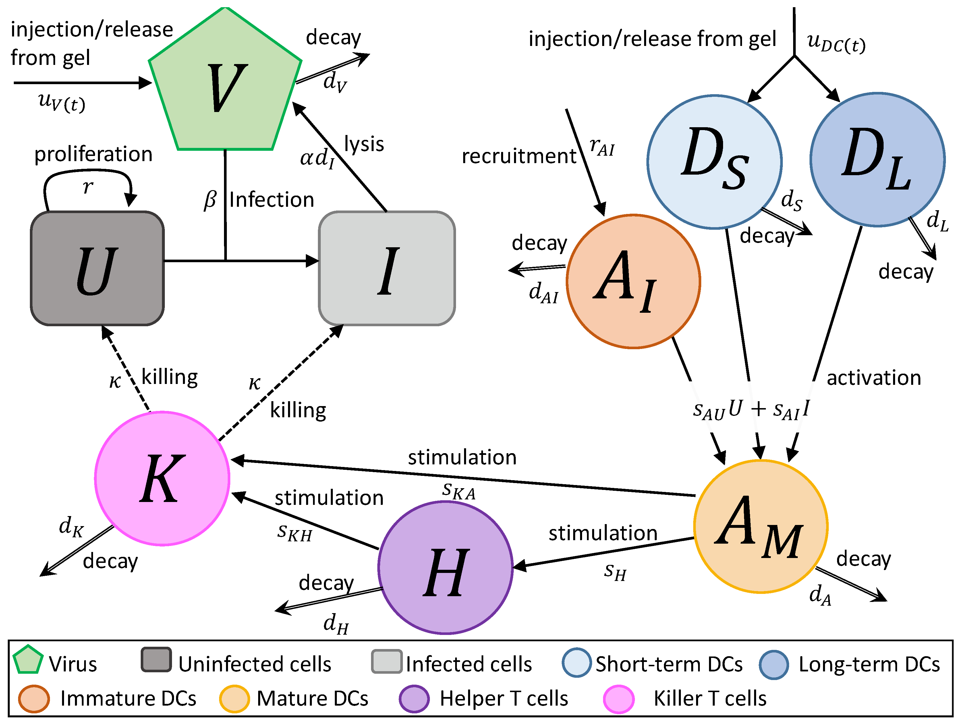
• In Equation (1), uninfected tumour cells, U, are growing at a rate described by a Gompertz function with proliferation rate r and carrying capacity L. Uninfected cells are infected by virus particles, V, at a frequency-dependent rate with rate constant $\beta$. Killer T cells, K, induce apoptosis in uninfected cells at a frequency-dependent rate with rate constant $\kappa$.
• In Equation (2), tumour cells become infected cells, I, at rate $\beta UV/N$. Infected cells lyse at rate $d_{I}I$, and, like uninfected cells, are killed at a frequency-dependent rate.
• In Equation (3), virus particles enter the system at rate $u_V\left(t\right)$, either by a single injection or release from the hydrogel. Virus particles decay at a rate $d_V$, and $\alpha$ new viruses are created through lysis.
• In Equation (4), short-term immature DCs, $D_S$, enter the system at a rate $(1-f)u_{DC}\left(t\right)$, either by a single injection or release from a hydrogel. They are then stimulated to become mature or activated APCs, $A_M$, at rate $s_{AU}$ or $s_{AI}$ due to the interaction with either uninfected or infected tumour cells. They decay at a fast rate $d_S$, where $d_S>>d_L$.
• In Equation (5), long-term immature DCs, $D_L$, enter the system at rate $f{u}_{DC}\left(t\right)$, where $u_{DC}\left(t\right)$ is the rate of injection or release from the hydrogel and f is the fraction of the initially loaded DCs that are long-term DCs, $0<f<1$. Similarly to short-term DCs, they become activated APCs at rate $s_{AU}$ and $s_{AI}$. These DCs decay slowly at rate $d_L$.
• In Equation (6), immature APCs, $A_I$, are recruited to the tumour site by infected cells at rate $r_{AI}I$. Immature APCs are then stimulated at the same rate as immature short-term and long-term DCs. The immature APCs decay at rate $d_{AI}$.
• In Equation (7), mature APCs are generated through the maturation of introduced long-term and short-term DCs and immature DCs recruited by uninfected tumour cells at rate $s_{AU}$ and infected tumour cells at rate $s_{AI}$. These cells decay at rate $d_A$.
• In Equation (8), helper T cels, H, are stimulated by mature APCs at a rate $s_H$. These cells decay at a rate $d_H$. We assume the rate APCs stimulate helper cells and helper cells stimulate killer cells is independent of antigen.
• In Equation (9), killer T cells, K, are activated by helper T cells and mature APCs at rates of $s_{KH}$ and $s_{KA}$, respectively. These cells either die or leave the tumour site at a rate $d_K$.

As the virus was administered either intratumourally or from the gel, there is no need to model the virus in the organs and blood (discussed by Jenner et al. [40]). Additionally, the influence of interferon-mediated antiviral immunity is not considered crucial. Note that this is the same killer T cell population that was considered by Jenner et al. [36], but this time the activation mechanism is modelled in more detail. The above model is similar to the model used by Kim et al. [35].

We consider two populations of immature dendritic cells ($D_L$ and $D_S$) in the initial administration as the in vitro release curve depicted a biphasic exponential decay profile for the DCs, see Section 3.1. We separated this population from the immature DCs already present in the mice, as we did not want to impose the assumption that the same separation in the survival rates would exist in this population.

If a gel is used to release the DCs and/or virus the initial conditions for system are

$$\begin{array}{cccc}U\left(0\right)=U_0,& I\left(0\right)=0,& V\left(0\right)=0,& D_L\left(0\right)=0,\\ D_S\left(0\right)=0& A_I\left(0\right)=0,& A_M\left(0\right)=0,& H\left(0\right)=0,& K\left(0\right)=0,\end{array}$$

(10)

where $U_0$ is the initial tumour size, whereas, for a single injection of virus or DCs, the initial conditions change to $V\left(0\right)=V_0,D_L\left(0\right)=f{D}_0$ and $D_S\left(0\right)=(1-f)D_0$ for the virus and DCs, where $V_0$ and $D_0$ are the initial number of viruses or DCs, respectively.

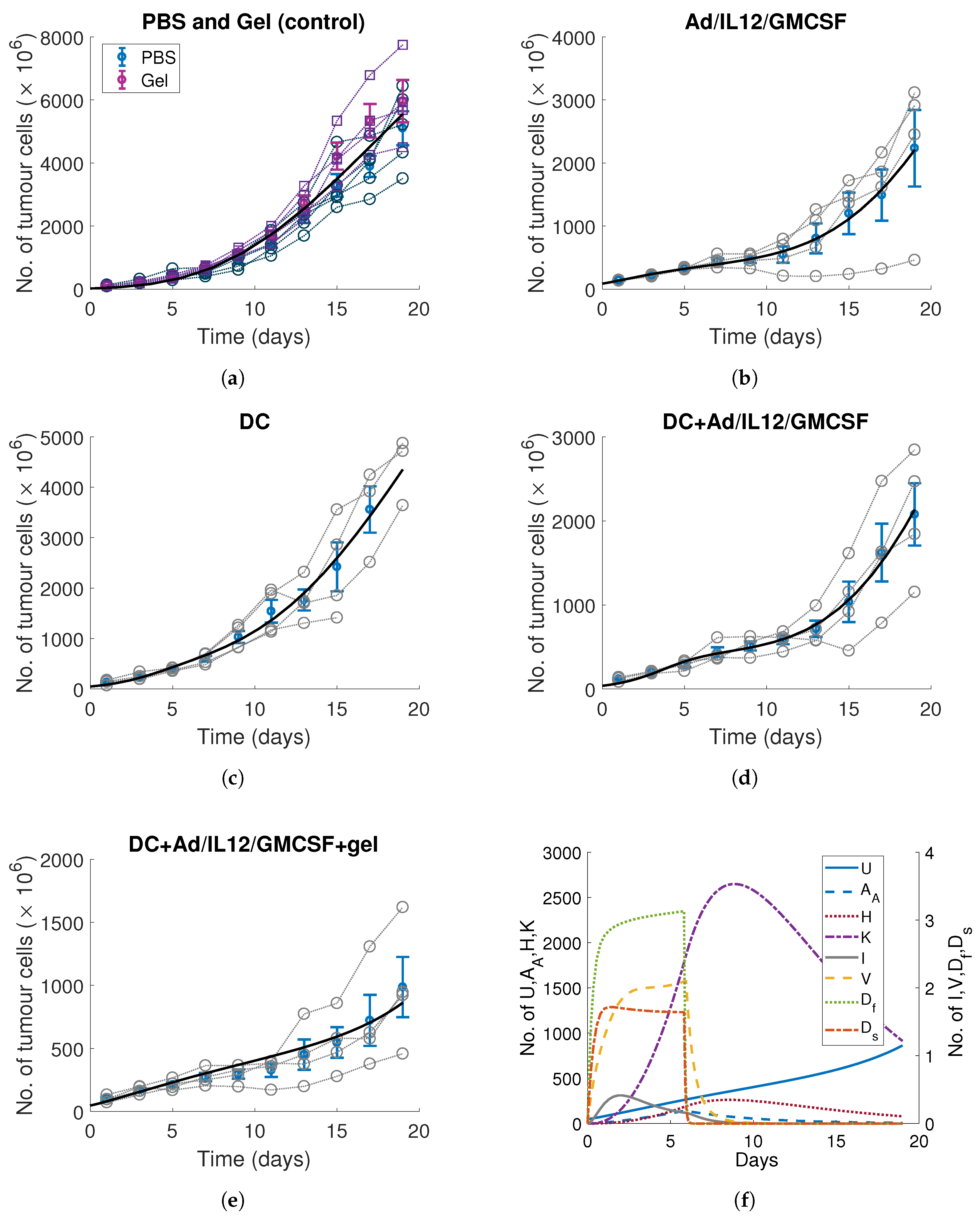
3. Calibrating Parameters to In Vitro and In Vivo Time-Series Measurements

To calibrate the parameters in Equations (1)–(9), we used the in vitro DC viability counts and in vivo tumour volume measurements of Oh et al. [10]. The release rate of DCs from the gel, $u_{DC}\left(t\right)$, and the decay rate for the long-term and short-term DCs, $d_L$ and $d_S$, were determined from DC viability counts with and without a degradable hydrogel [10]. We then fixed certain parameters to their values obtained in our previous work [36] where we optimised tumour volume measurements for the Ad/IL12/GMCSF virus based on experiments by Choi et al. [13]. The remaining parameters were then optimised to the in vivo tumour time-series measurements from [10] under treatment with a single injection of either DC, Ad/IL12/GMCSF or DC+Ad/IL12/GMCSF and treatment with a degradable hydrogel containing DC+Ad/IL12/GMCSF.

3.1. DC Release-Profile and Decay Rates

Oh et al. [10] counted the number of viable DCs after a single injection released from a gel over 6 days. To fit these measurements, we fixed $U=I=V=A_I=A_M=H=K$ in Equations (1)–(9) as no tumour cells, immune cells or virus were present, and then optimised the decay rates of the long-term and short-term DCs, $d_L$ and $d_S$, to the DC count after a single injection, see Figure 2a and

Table 1. Parameter values obtained from fitting the release rate of the DCs and the short-term and long-term decay rates of the DCs to the in vitro viable DC count, see Figure 2.

Parameter	Units	Description	Value
$d_S$	day${}^{-1}$	decay rate of short-term immature DCs	1.562
$d_L$	day${}^{-1}$	decay rate of long-term immature DCs	0.318
f	dimensionless	proportion of short-term injected/released DCs	0.325
$a_D$	DCs/day${}^2$	gradient of release rate	9.725 $\times {10}^4$
$b_D$	DCs/day	constant release rate	1.463 $\times {10}^5$

. We initially considered a single decay rate for the injected immature DCs and found that the long-term model prediction was a significant underestimation. The data seems to suggest a fraction of the injected DCs live longer and contribute to a slower population decline after the first few days. As the DCs are derived from bone marrow, the difference in decay rates may be a result of heterogeneity imposed from the progenitor cell lineages that generate the DCs [41,42]. We, therefore, assumed that there are both long-term and short-term surviving immature DCs in the injected population. This biphasic decay rate is evident in other studies of bone marrow- or monocyte-derived DCs [43]. The decay rate could be modelled more accurately with a age-structured partial differential equation system, but due to the limited data, we decided this was not necessary.

From the measurements of the DCs released from the hydrogel [10], we then obtained the release-rate function $u_{DC}\left(t\right)$. Oh et al. [10] used a gelatin-hydroxyphenyl propionic acid (GHPA)-based hydrogel that can easily be manipulated to achieve appropriate hydrogel properties such as gelatin time, mechanical stiffness and degradation rate. Previous experiments with this hydrogel showed that gel weight decreases linearly over time [44], implying that the gel degrades linearly. Taking the forward finite difference approximation of the data revealed an approximately linear, increasing rate of change for the DCs released from the gel. As we chose not to model the gel-release mechanics, we assumed that a linear function would be sufficient to capture the gel-release rate.

We fixed $d_L,d_S$ and f to the values obtained for Figure 2a and assumed $u_{DC}\left(t\right)$ would be

$$u_{DC}\left(t\right)=\left\{\begin{array}{cc}{a}_{D}t+b_D& D_I>0,\\ 0& D_I=0,\end{array}\right.$$

(11)

where $a_D$ is the gradient of $u_{DC}\left(t\right)$; b is the initial release rate from the gel (i.e., $u_{DC}\left(0\right)=b_D$); and $D_I$ is the number of DCs in the gel, where $d{D}_I/dt=-u_{DC}\left(t\right)$ and $D_I\left(0\right)=2.5\times {10}^6$. Qualitatively, $a_D$ describes the increasing speed that treatment is released from the gel as a function of time, and $b_D$ describes the initial rate at which treatment is released when the gel is first put into the solution bath. See Figure 2b and Table 1 for the results. From the fitted parameter values, we obtain the approximate time that the gel degrades as $t_r=5.945$ days, which matched the observations of Oh et al. that by day 6 the gel had completely degraded.

3.2. Tumour, Immune and Viral Parameters

To obtain remaining parameter estimates for the model, we sequentially optimised the tumour time-series measurements of Oh et al. [10] for PBS, gel, Ad/IL12/GMCSF, DC+Ad/IL12/GMCSF and DC+Ad/IL12/GMCSF+gel. To reduce the degrees of freedom in the model, the parameters $\alpha ,d_I,d_V,d_A,d_H,d_K,$$s_A,s_{KA},s_H$ and $s_{KH}$ were fixed to the values obtained from optimising tumour growth under Ad/IL12/GMCSF treatment in Jenner et al. [36]. The remaining parameters were obtained by sequentially fitting sub-models of Equations (1)–(9), where fitted parameter values were fixed for higher level models in accordance with the different treatments investigated.

Table 2. Experiment-specific optimisation conditions for the measurements of Oh et al. [10]. Equations used to optimise each experiment are listed along with the state variables considered and parameters fitted or fixed. Some parameters were fixed to previous optimisation work in Jenner et al. [36].

Experiment
	PBS & Gel	Ad/I/G	DC	DC+Ad/I/G	DC+Ad/I/G+Gel
Relevant equations	Equation (1)	Equation (1)	Equation (1)	Equation (1)	Equation (1)
		Equation (2)		Equation (2)	Equation (2)
			Equation (3)	Equation (3)	Equation (3)
			Equation (5)	Equation (5)	Equation (5)
			Equation (4)	Equation (4)	Equation (4)
				Equation (6)	Equation (6)
		Equation (7)	Equation (7)	Equation (7)	Equation (7)
		Equation (8)	Equation (8)	Equation (8)	Equation (8)
		Equation (9)	Equation (9)	Equation (9)	Equation (9)
Variables	U	U,I,V	U	U,I,V	U,I,V
		A,H	AI,AM, H	AI,AM, H	AI,AM, H
		K	K	K	K
Parameters fit	r,L,U0	β,U0	sAU,U0	rAI,SAI,U0	aV,bV,U0
		k	k		sAU
Parameters fixed to Table 1 and Table 3	-	r,L	r,L	r,L,β	r,L,β
			dS,dL,dAI	dS,dL,dAI,κ	dS,dL,aD,bD
					dAI,rAI,sAI,k
Parameters fixed from [36]		dV,α,sH,dH	sH,dH	dV,α,sH,dH	dV,α,sH,dH
		dI,sA,dA	dA	dI,sAU,dA	dI,sAU,dA
		sKH,sKA,dK	sKH,sKA,dK	sKH,sKA,dK	sKH,sKA,dK

gives a summary of the fitting algorithm, with parameter values in

Table 3. Parameter estimates from the sequential optimisation of the model following the algorithm in Table 2 to the experimental measurements in [10]. Certain parameters were fixed to their value in [36], and this is indicated in the table. Parameters that were fit for a particular experiment have their values in bold. Note that Ad/IL12/GMCSF has been shortened to Ad/I/G.

	Param	Units	Description	PBS& Gel	Ad/I/G	DC	DC + Ad/I/G	DC + Ad/I/G + gel
Fit	$d_{AI}$	day${}^{-1}$	Immature DCs decay rate			1.562	1.562	1.562
	L	cells $\times {10}^6$	carrying capacity	13572	13572	13572	13572	135720
	r	day${}^{-1}$	growth rate	0.1045	0.1045	0.1045	0.1045	0.1045
	$U_0$	cells $\times {10}^6$	initial tumour size	20.35	85.90	85.90	85.90	47.45
	$\beta$	day${}^{-1}$	infection rate	-	0.7295	-	0.7295	0.7295
	$\kappa$	day${}^{-1}$	killing rate	-	0.8225	0.218147	0.3626	0.3626
	$s_{AU}$	day${}^{-1}$	APC activation rate by U	-	-	0.001047	0.0022	0.05278
	$r_{AI}$	day${}^{-1}$	recruitment rate of $A_I$	-	-	-	0.0192	0.0192
	$s_{AI}$	day${}^{-1}$	APC activation rate by I	-	-	-	0.0011	0.0011
	$a_V$		linear release slope (virus)	-	-	-	-	0.33791
	$b_V$		initial linear release (virus)	-	-	-	-	2.35971
[36]	$\alpha$	virus $\times {10}^{10}$	viral burst size	-	3500	-	3500	3500
	$d_I$	day${}^{-1}$	burst rate	-	1	-	1	1
	$d_V$	day${}^{-1}$	viral decay rate	-	2.3	-	2.3	2.3
	$d_A$	day${}^{-1}$	decay of mature APCs	-	0.23	0.23	0.23	0.23
	$d_{AI}$	day${}^{-1}$	decay of immature APCs	-	1.562	1.562	1.562	1.562
	$d_H$	day${}^{-1}$	decay of helper T cells	-	0.23	0.23	0.23	0.23
	$d_K$	day${}^{-1}$	decay of killer T cells	-	0.35	0.35	0.35	0.35
	$s_A$	day${}^{-1}$	APC activation rate	-	1.2	-	7.1	7.1
	$s_{KA}$	day${}^{-1}$	APC activatet killer T cell	-	7.1	7.1
	$s_H$	day${}^{-1}$	helper T cell activation	-	0.78	0.78	0.78	0.78
	$s_{KH}$	day${}^{-1}$	helper T cell activate K	-	1.6	1.6	1.6	1.6

.

As a control, Oh et al. [10] measured the tumour growth under a single injection of PBS and an empty gel. We assumed that the underlying tumour growth in both of these experiments should be identical and fit the growth rate, r; carrying capacity, L; and initial tumour size, $U_0$, to both data sets, fixing $I=V=A_I=A_M=H=K=0$ in Equations (1)–(8), see Figure 3a.

Following the control experiments, Oh et al. [10] measured the tumour size under a single injection of Ad/IL12/GMCSF. As there was no injection of immature DCs in this experiment, we assumed the immune stimulation would be driven solely by the injected virus with the effects of endogenous DCs negligible, i.e., we fixed $D_S=D_L=A_I=0$. Under this assumption, we removed any activation of APCs by uninfected tumour cells, and modelled APC stimulation as directly relating to infected cells I, i.e., $s_{AI}I(A_I+D_L+D_S)=s_{AI}I$. The remaining parameters of the model describing the infection rate of the virus, $\beta$; the killing rate of the killer T cells, $\kappa$; and the initial tumour size, $U_0$, were optimised, see Figure 3b.

Oh et al. [10] then measured tumour growth under a single injection of $2.5\times {10}^6$ immature DCs. As there was no virus present, we fixed $I=V=0$. The decay rate for immature APCs, $d_{AI}$, was fixed to the short-term DC decay rate, $d_S$, as we assumed that any recruited immature APCs would not reside at the tumour site for long. The parameters describing the stimulation rate of immature APCs, $s_{AU}$; the killing rate of killing cells, $\kappa$; and the initial tumour size were optimised and fixed for subsequent optimisations, see Figure 3c.

Following this, Oh et al. [10] combined a single injection of Ad/IL12/GMCSF with a single injection of immature DCs. Fixing the previous fit parameters, we optimised the kinetics for the activation of immature APCs and DCs using the full model in Equations (1)–(9). Optimising the rate that infected cells recruit inactivated APCs $r_{AI}$, the stimulation of immature APCs $s_{AI}$ and initial tumour size $U_0$ gave the model curve in Figure 3d.

The final experiment of Oh et al. [10] measured the tumour volume after a gel loaded with Ad/IL12/GMCSF and immature DCs was injected adjacent to the tumour. Using these measurements, we obtained the release profile for the virus from the gel $u_V\left(t\right)$. Fixing the release profile of the immature DCs from the gel, $u_{DC}\left(t\right)$, to the profile determined in Section 3.1 and all parameters to the values for the DC+Ad/IL12/GMCSF experiment, we assumed the release rate for the virus would be linear, and the time of release $t_r$ would be equivalent to that obtained for the DCs, $t_r=5.945$ days,

$$u_V\left(t\right)=\left\{\begin{array}{cc}{a}_{V}t+b_V,& \mathrm{for}t\le t_r\\ 0& otherwise\end{array}\right.$$

where $a_V>0$ and $b_V\ge 0$. The value of $b_V$ was obtained by fixing the initial amount of virus as $V_0=2\times {10}^{10}$ and integrating $u_V\left(t\right)$. Additionally, we obtained an upper and lower bounds of $a_V$ using the condition that $u_V\left(t\right)$ is an increasing function. Optimising the release function parameter $a_V$ was not sufficient, and a fit could only be obtained when the activation rate of APCs by uninfected cells was also allowed to vary. The resulting fit is in Figure 3e and the parameter values are in Table 3. The model dynamics for this experiment are plotted adjacent in Figure 3f.

All parameter optimisations were undertaken using a least-squares nonlinear fitting algorithm “lsqnonlin” in MATLAB2017a. The termination tolerance was $1\times {10}^{-6}$. The maximum number of function evaluations was fixed as $100\times$ number of parameters. The maximum number of interactions for each fit was 400. The solver ode45 was used to solve the model. The model was fit simultaneously to the set of individual mouse data for a particular experiment. When solving Equations (1)–(9) numerically, T was replaced by $T+ϵ$ for $ϵ=0.001$ to avoid a singularity as $T\to 0$. The goodness of fit statistics have been reported in

Table 4. Goodness of fit statistics for the optimisation of the mathematical model Equations (1)–(9) with the experiments in Figure 3 following the optimisation algorithm in Table 2.

	Residual	Coefficient of	Pearson’s Correlation
	Norm	Determination (${\mathit{R}}^2$)	Coefficient
PBS and gel	33,688	0.8998	0.9487
Ad/IL12/GMCSF	10,905	0.6465	0.8041
DC	11,931	0.8980	0.9441
DC+Ad/IL12/GMCSF	7659.4	0.7785	0.8830
DC+Ad/IL12/GMCSF+gel	5249.7	0.5926	0.7736

.

It is evident visually in Figure 3 and from the goodness of fit measurements (Table 4) that our model and the sequential fitting algorithm we used in Table 2 provide a reliable representation of the data. From the population dynamics in Figure 3f, it is clear that the immune response is driven by a large increase in helper T cells coinciding with mature APCs. This then prolongs the killer immune cell population’s survival. From the model, it does appear though that it is the initial viral infection that drives the tumour population down significantly.

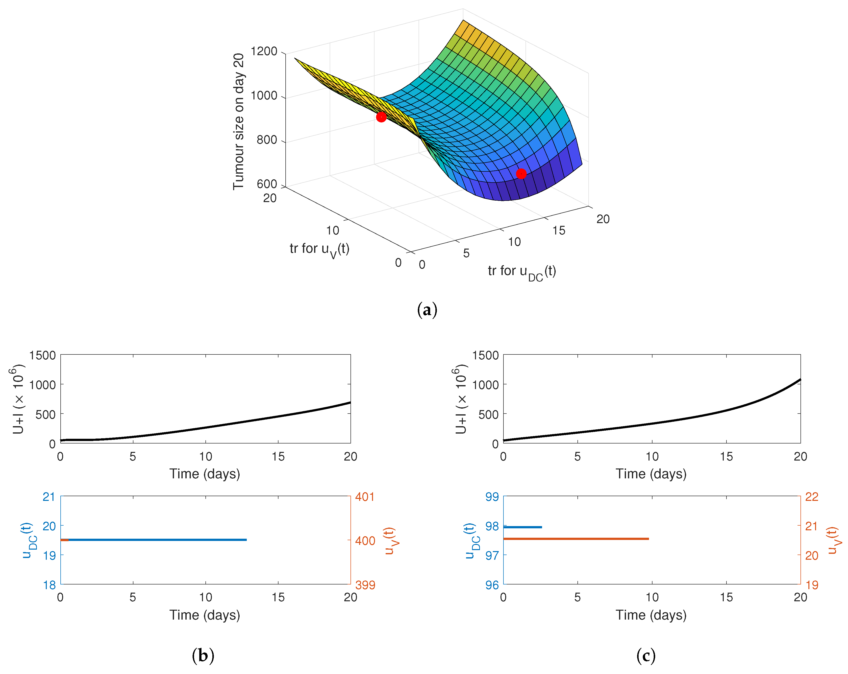
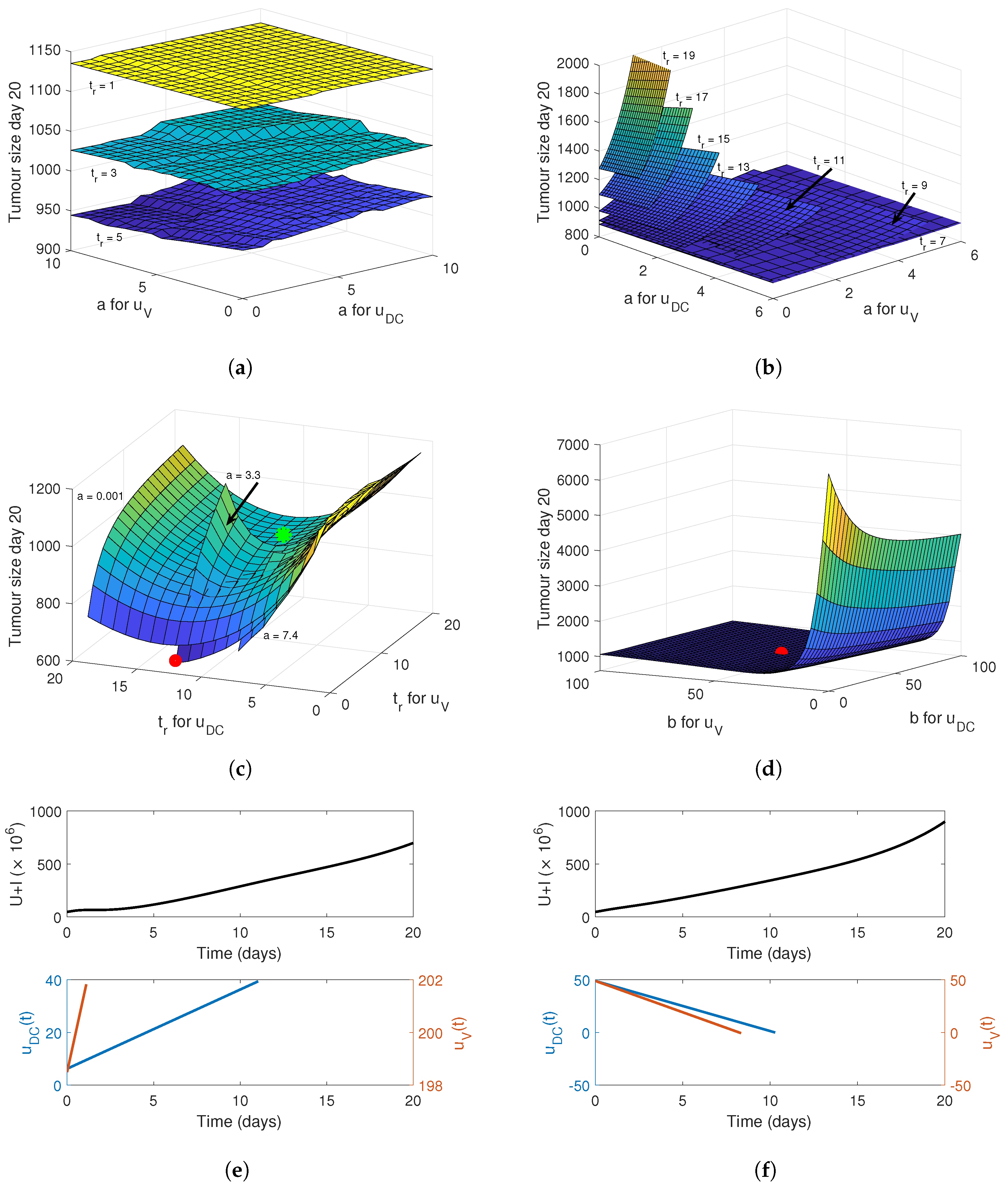
4. Optimising the Gel Release Profile

Oh et al. [10]’s gel-based medium improved the therapeutic efficacy of the DC+Ad/IL12/GMCSF treatment and reduced the tumour volume to 1005.9 mm${}^3$ by day 20, see Figure 3e. It may be possible to further improve this treatment through the manipulation of the gel-release profile, $u_{DC}\left(t\right)$ and $u_V\left(t\right)$. To investigate this, we considered gel-release profiles that were constant, linear and sigmoidal. We chose these functions as they had increasing complexity in their time dependence and were qualitatively similar for certain parameter regimes. Many therapeutics require a constant release rate for varying durations [45], and while this is difficult to achieve, there are several examples [46,47,48]. In comparison, variable drug release rates, such as linear and sigmoidal curves are more obtainable [49,50,51,52].

We, therefore, define three generalised release rate functions for $u_{DC}\left(t\right)$ and $u_V\left(t\right)$: constant $f_c\left(t\right)$, linear $f_l\left(t\right)$ and sigmoidal $f_s\left(t\right)$. These have the forms

$$\begin{array}{cc}\hfill f_c\left(t\right)& =C,\hfill \end{array}$$

(12)

$$\begin{array}{cc}\hfill f_l\left(t\right)& =at+C,\hfill \end{array}$$

(13)

$$\begin{array}{cc}\hfill f_s\left(t\right)& =\frac{L}{1+e^{-k(t-x_0)}},\hfill \end{array}$$

(14)

where C is the constant release rate, a is the gradient of the linear release, k is the steepness of the sigmoidal release rate, $x_0$ is the midpoint of the sigmoidal function and L is the maximum sigmoidal release rate. We impose the constraint that the total virus and DCs released from the gel over $t_r$ days must be equal to $V_0$ and $D_0$, i.e.,

$$V_0={\mathsf{\int }}_0^{t_r}{u}_V\left(s\right)ds,D_0={\mathsf{\int }}_0^{t_r}{u}_{DC}\left(s\right)ds.$$

(15)

Fixing all parameter values not related to the release curves to those in the DC+Ad/I/G+gel column in Table 3, we simulated the tumour size up to day 20 using Equations (1)–(9) for the different release profiles $f_c\left(t\right),f_l\left(t\right)$ or $f_s\left(t\right)$ for $t\le t_r$, and 0 otherwise.

4.1. Constant Release Profile

Assuming both virus and DCs are released from the gel at a constant rate, $f_c\left(t\right)$ in Equation (12), and integrating and simplifying using Equation (15) gives

$$u_V\left(t\right)=\frac{V_0}{t_r},u_{DC}\left(t\right)=\frac{D_0}{t_r}.$$

(16)

We can then simulate the effect of different release periods, $t_r$, for virus and DCs. The tumour volume on day 20 as a function of the release period is plotted in Figure 4a. The surface has a global minimum tumour size of 689.24 mm ${}^3$, which corresponds to a 13-day release period of DCs and a single day for the virus.

To illustrate the tumour growth dynamics under different constant release profiles, model simulations are plotted in Figure 4b,c, corresponding to the red points on the surface plot in Figure 4a. There is a decrease in the initial gradient of the tumour growth in Figure 4b compared to Figure 4c, which in turn allows for a more gradual linear tumour growth over the period of 20 days. This suggests that releasing the virus rapidly and then slowly releasing the immature DCs over 13 days, reduces the growth rate of the tumour by providing continual stimulation for the immune system.

4.2. Linear Release Profile

Assuming both virus and DCs are released from the gel at a linear rate, $f_l\left(t\right)$ in Equation (13), which is increasing, applying the constraint in Equation (15) gives

$$u_V\left(t\right)=a\left(t-\frac{t_r}{2}\right)+\frac{V_0}{t_r},u_{DC}\left(t\right)=a\left(t-\frac{t_r}{2}\right)+\frac{D_0}{t_r}.$$

(17)

To investigate whether there was an optimal increasing linear release rate, we initially fixed $t_r$ as common for virus and DCs and varied the gradient of the release curve a, which was bounded by $0<a<2A_0/t_r^2$ so as to be strictly positive and increasing. The resulting tumour size on day 20 is plotted in Figure 5a,b. As $t_r$ increases from 1 day to 5 days, the overall tumour size decreases irrespective of the choice of a. However, after a release period of $t_r=6$ days, the minimum achievable tumour size at day 20 increases and so does the dependence of the tumour size at day 20 on the steepness of the release rate a. A minimum tumour size of 887 mm ${}^3$ was achieved for $t_r=11$ days and $t_r=13$ days when $a=0$. In other words, if the release time is common for DCs and virus, the optimal linear release curve is approximately constant.

We then numerically simulated the increasing linear release rate with $t_r$ varying for virus and DCs and fixed $a=0.001,3.3$ and $7.4$, see Figure 5c. Qualitatively, the dependence on the value of $t_r$ for $u_{DC}\left(t\right)$ and $u_V\left(t\right)$ is similar to that of the constant release profile in Figure 4a. A minimum tumour volume of 628.4 mm ${}^3$ was achieved for an interval of a between 3.3 and 4.6 for $t_r=1$ for the virus and $t_r$ between 11 and 13 for DCs. This suggests that it is possible to obtain an optimal efficacy with the linear release function, but only when the release time of the constituents are separated.

Although the gel-release mechanisms measured by Oh et al. [10] had an increasing gradient, it is worth considering how effective a treatment would be when released at a decreasing linear rate. A decreasing linear function crosses $u_{DC}\left(t\right)=0$ or $u_V\left(t\right)=0$ when $t=-b/a$. As this can occur before or after 20 days, we use this to constrain the release curve by fixing the total drug released between 0 and $-b/a$ days equal to $V_0$ and $D_0$. Integrating and simplifying gives

$$u_V\left(t\right)=\frac{-b^2}{2V_0}t+b,u_{DC}\left(t\right)=\frac{-b^2}{2D_0}t+b,$$

(18)

where b is the initial release rate. Note that this means the gel releases until $-b/a$ days, or $2V_0/b$ for the virus and $2D_0/b$ days for DCs. This can be outside the window of the evaluated time-frame and as such may lead to less virus and DCs released than $V_0$ and $D_0$.

Simulating a common value of b for virus and DCs gives the tumour volume on day 20 in Figure 5d. The tumour volume depends on the value of the initial release rate for the virus with larger values of b resulting in the lowest tumour volume. Note that when b increases, the release time $t_r$ decreases, so the optimal tumour burden for the decreasing linear release is achieved when b is large enough so that the total amount of $D_0$ and $V_0$ is released within 20 days. Interestingly, we do not see a dependence on the time frame in which the treatment is released (in contrast to the cases of constant release and linear increase). For the linearly decreasing release, the duration of the release is negligible, even considering separate release rates for virus and DCs. The numerical global minimum for the decreasing linear release rate is 815.5 mm ${}^3$. The tumour dynamics for different linear release curve are plotted in Figure 5e,f.

4.3. Sigmoidal Release Profile

The final release curve considered was a sigmoidal function $f_s\left(t\right)$, given by Equation (14). Integrating and simplifying using the constraint in Equation (15) gives

$$u_V\left(t\right)=\frac{k{V}_0}{\left(ln\left(\frac{1+e^{-k(t_r-x_0)}}{1+e^{k{x}_0}}\right)+t_{r}k\right)\left(1+e^{-k(t-x_0)}\right)},u_{DC}\left(t\right)=\frac{k{D}_0}{\left(ln\left(\frac{1+e^{-k(t_r-x_0)}}{1+e^{k{x}_0}}\right)+t_{r}k\right)\left(1+e^{-k(t-x_0)}\right)}.$$

(19)

We imposed additional constraints on the sigmoidal function so that the function was always positive, i.e., when $k>0$, the function within the “ln” would always be positive, and when $k<0$, the denominator was always negative.

Assuming initially that the characteristics of the release curve for virus and DCs are equivalent, gives the tumour size at day 20 in Figure 6a for a release period of 5 days, 9 days and 13 days. The sign of k determines whether the sigmoidal function is increasing or decreasing. This explains the clear dynamical switch at $k=0$. For increasing sigmoidal release curves ($k>0$), the tumour size is minimised when the mid-point $x_0$ is larger. The overall minimum tumour size is achieved for increasing release curves when the midpoint is decreased below zero. The release period $t_r$ influences the minimum achieved with $t_r=9$ achieving a lower tumour volume than $t_r=5$, and the planes associated with $t_r=9$ and $t_r=13$ approaching the same limit for $x_0\to 0$.

Investigating this further, the release time $t_r$ was fixed to 9 days and the value of k varied for virus and DCs for $x_0=-1,1$ and 3, see Figure 6b. Lower values of k for the DCs reduced the tumour volume when the midpoint $x_0$ was positive. As $x_0$ decreases, the variance in the plane reduces, and we see, overall, the minimum tumour burden is achieved irrespective of k for $x_0=-1$.

Simulating varying $x_0>0$ for virus and DCs and fixing $k=-1,1$ and 3, we see that the value of the midpoint needed to minimise the tumour burden depends most heavily on the midpoint for $u_{DC}\left(t\right)$, Figure 6c. If $k>0$, then a lower $x_0$ is needed, whereas the opposite is exhibited if $k<0$. Unsurprisingly, simulating the sigmoidal function for fixed values of $k=1$ and $x_0=1$ and varying $t_r$ for DCs and virus, we have similar dynamics to the linear and constant release curves, see Figure 6d. For an increasing sigmoidal function, the optimal tumour size is obtained when the virus is released quickly and the DCs have an extended release. Two model simulations are provided in Figure 6e,f to demonstrate the different sigmoidal release functions considered.

4.4. Implementing a Genetic Algorithm to Determine the True Optimal Release Curves

In the previous sections, the gel-release dynamics have been qualitatively linked with the tumour burden on day 20. To determine the optimal parameter sets for the constant, linear and sigmoidal dosage functions, the tumour volume on day 20 was minimised under each release profile using Matlab’s genetic algorithm function ga [53]. Genetic algorithms are heuristic global optimisation routines inspired by natural selection that are frequently employed to estimate parameters in computational biology models. They have previously been applied to study optimal dosing routines in immunology [54,55] and combined oncolytic virotherapy and immunotherapy [29].

The tumour growth under the optimised constant, linear and sigmoidal release curves for virus and DCs are pictured in Figure 7. The parameter values from the genetic algorithm for each optimal release curve are given in

Table 5. Optimised parameter values for the constant $f_c$, linear $f_l$ and sigmoidal $f_s$ release curves (Equations (12)–(14)) for Ad/IL12/GMCSF and immature DCs from a gel. The virus and DCs were allowed to have individualised curves. Figure 7 is a plot of the tumour volume under the five optimised curves.

		Constant	Linear (Increasing)		Sigmoidal
		${\mathit{t}}_{\mathit{r}}$	${\mathit{t}}_{\mathit{r}}$	$\mathit{a}$	${\mathit{t}}_{\mathit{r}}$	$\mathit{k}$	${\mathit{x}}_{\mathbf{0}}$
Ad/IL12/GMCSF	$u_V\left(t\right)$	0.1261	0.1252	14.9893	0.05	9.2789	−6.0499
DCs	$u_{DC}\left(t\right)$	13.7732	13.1629	2.8866	13.6311	9.1951	−8.3333

. The constraints applied for the numerical simulations were also applied here for the different release curves. The optimal decreasing linear release curve has not been plotted as we know from the numerical simulations that it did not achieve a significant global minimum. Additionally, we found that the decreasing sigmoidal function’s optimal parameters qualitatively matched that of the increasing sigmoidal function.

Figure 7c shows that all three optimised release curves are able to reduce the tumour burden below the average size from Oh et al.’s experiments [10]. The dynamics of the immature APC population ($D_L+D_S+A_I$) are similar for the constant and sigmoidal release curves, see Figure 7a, whereas the optimal linear release profile delays the initiation of the APC accumulation. As the virus dynamics are the same for the three release curves (Figure 7b), this suggests that the delay on the immature APC population expansion causes the decrease in tumour size under the optimised linear release therapy in Figure 7c.

Overall, the parameters returned from the genetic algorithm matched the qualitative results of the numerical investigation for the constant and linear release functions. Both release curves required less than a day for the virus release and approximately 13 days for the DCs. The steepness of the linear curve a was much higher for the virus than the DCs, with the DC’s value of a close to that plotted in Figure 5c. The sigmoidal release curve had the same dependence on the release curves for viruses and DCs as the constant and linear release period. Interestingly, the midpoint for both functions was significantly negative, meaning the curve would be similar to an increasing linear release profile. These results all suggest that the added complexity of the sigmoidal function with the time-varying gradient does not improve the efficacy of the gel-release mechanism.

5. Discussion

In this work, we developed a system of ordinary differential equations for the sustained release of virus and immature dendritic cells from a gel and the resulting interaction with a population of tumour cells and immune cells. Using our model, we recreated the in vitro and in vivo experiments of Oh et al. [10] (Figure 2 and Figure 3). Using the calibrated model, we have been able to provide insight into how the gel-release profile may be optimised to improve treatment.

In the sequential fitting, attributes of the model were calibrated to the tumour response to combined Ad/IL12/GMCSF and immature DC therapy (Figure 3). To optimise the model to the Ad/IL12/GMCSF treatment of Lewis Lung Carcinoma (LLC) tumours by Oh et al. [10], we fixed most parameters to values obtained from our previous optimisation of the Ad/IL12/GMCSF treatment of melanoma [36], fitting only the virus infection rate, $\beta$, and killer T cell killing rate, $\kappa$ (see Figure 3b). Both these parameters decreased for the treatment of LLC tumours compared to melanoma, suggesting that different tumour cells lines will ultimately result in different virus and immune characteristics.

From the optimisation of the single immature DC injection (Figure 3c) and the combined DCs+Ad/IL12/GMCSF injection (Figure 3d), we found that immature APCs are stimulated more rapidly by infected as opposed to uninfected cells, parameters $s_{AI}$ and $s_{AU}$, respectively. Additionally, we note that the killing rate, $\kappa$, decreased for Ad/IL12/GMCSF alone, compared to DC+Ad/IL12/GMCSF. We hypothesise that the addition of immature DCs results in a heightened antitumour immune response, which results in a “division of resources” between the antitumour and antiviral immune response.

Oh et al. [10] reduced the tumour size by 50% on day 20 by using a GHPA hydrogel to release the DC+Ad/IL12/GMCSF treatment (Figure 3e). Using our calibrated model (Table 3), we numerically investigated alternative gel-release profiles to determine whether we could reduce the tumour burden further. Conserving the total amount of virus and DCs released from the gel, we first considered a constant gel-release profile. Simulating different release periods, $t_r$, for the virus and DCs we found a minimum tumour size is attainable when the virus is released over a day, and the DCs are released for 13 days (Figure 4). This suggests that an initial burst of virus reduces the tumour volume through infection and stimulates an immune response that, under a prolonged constant release of DCs from the gel, results in a significantly reduced tumour volume.

A natural extension was then to examine the tumour volume under different linear releases. If the release period, $t_r$, is fixed for both the DCs and the virus, then release periods between $t_r=5$ to 14 days reduce the tumour burden most significantly (Figure 5a,b). The global optimal of this regime occurs when $a\approx 0$, i.e., a constant release profile, suggesting that the optimal protocol is constant administration if release periods for the virus and DCs cannot be distinct. For unique release times, the optimal release period is similar to the constant release profiles: virus released rapidly and the DCs released slowly over time (Figure 5c). Overall, the gel designed by Oh et al. performed optimally and there are many increasing linear release profiles that would have performed significantly worse.

Considering the more complex sigmoidal gel-release profile, we found that the tumour burden was reduced when the midpoint was below 0 and the curve was an increasing function (Figure 6a,b). In other words, when the gradient of the release rate was reducing and tending towards a constant release profile. Furthermore, explicitly increasing the steepness, k, of the sigmoidal curve always increased the tumour size (Figure 6b,c). Unsurprisingly, the optimal release period for viruses and DCs was qualitatively similar to that of the constant and linear release periods (Figure 6d), implying that it is primarily the release period that optimises the treatment irrespective of the release curve.

Implementing a genetic algorithm, we were able to determine the true optimal constant, linear and sigmoidal release curves (Table 5 and Figure 7). Unsurprisingly, the optimal release curves each had a short release time for the virus and an extended release time of 13 days for the DCs. Comparing the impact of the different optimal release curves (Figure 7c), we see that the difference in the tumour size was minimal. Although the optimised linear release curve reduced the tumour size the most, all release curves improved the treatment by a similar amount. This suggests that extending the complexity of the release mechanisms may not be necessary, as a constant release curve performs almost as well as a linear release curve, and the optimised sigmoidal curve is more constant than sigmoidal. Additionally, this also suggests that for the constraints considered on the release curves it is not possible to optimise the gel so that the tumour is completely eradicated.

Previously, Barish et al. [38] optimised the scheduling of discrete doses of oncolytic virus and DCs. They showed that higher doses of DCs were needed to result in a robust optimised therapy. The fact that our results suggest the need for sustained release of DCs complements their findings and demonstrates that therapy can be optimised when the timing of DC administration is optimal. Our results also align with the results of Wares et al. [37], where they showed using a calibrated model that it is more effective to treat a tumour with immunostimulatory oncolytic viruses first and then follow up with a sequence of DCs than to alternate oncolytic virus and DC injections.

A limiting assumption of this work is that the complex gel mechanics are modelled phenomenologically. As the goal was to investigate the effect of changing the function $u_{DC}\left(t\right)$, we believe it is not necessary to model the gel-release kinetics explicitly and, as qualitatively the model formulation for the measurements with and without the gel is able to capture the model dynamics (see Figure 2), this was a suitable simplification. Future work, however, would look to develop a more appropriate realisation of the gel kinetics and investigate mechanistically the optimal release profile. Another simplification in the model is that the rate at which immune cells are stimulated is independent of the antigen type. In reality, immune cells are antigen specific [18] with either tumour–antigen- or virus–antigen-specific cells. Future extensions of this work could consider two populations of immune cells similar to the work of Mahasa et al. [56] and investigate further why optimised gel-release profiles require an extended DC release.

Using a system of ODEs, we were able to replicate the experimental conditions of DC+Ad/IL12/GMCSF therapy and determine possible improvements to the gel-release profile. This model can be applied to other viro-immunotherapies that aim to activate the adaptive antitumour immune response. As we only consider simple formulations for the gel-release rate, this model is easily translatable to other sustained-release delivery systems where the release functions $u_V\left(t\right)$ and $u_{DC}\left(t\right)$ may or may not be known. Our results on the optimal timing of virus and DC treatment provide insight into how future viro-immunotherapies using DCs need to be designed. From this work, we present a mathematical model that can be used to provide insight into other oncolytic virotherapies or viro-immunotherapies and predict the impact of sustained-delivery systems.

6. Conclusions

The mathematical model of tumour cell, virus and immune interactions derived in this study is a good representation of the response to viro-immunotherapy. We have shown how a sequential optimisation of experimental data provides insight into the underlying biology of the interaction. From our numerical optimisation of the gel developed by Oh et al. [10], we were able to show which key characteristics optimised or reduced the gel’s efficacy. We found that if the virus is released instantaneously and the DCs are released over 13 days, then the tumour size under treatment can be improved. In turn, we were able to show that additional complexity in the gel-release profile does not add any improvement to the treatment outcome. Ultimately, to improve this treatment dramatically, it is not sufficient to solely manipulate the gel: more would need to be done to change the underlying efficacy of the virus and immune response to ultimately improve treatment.

References

1. Ta, H.T.; Dass, C.R.; Dunstan, D.E. Injectable chitosan hydrogels for localised cancer therapy. J. Control. Release 2008, 126, 205–216. [Google Scholar] [CrossRef] [PubMed]
2. Sahu, P.; Kashaw, S.K.; Sau, S.; Kushwah, V.; Jain, S.; Agrawal, R.K.; Iyer, A.K. pH responsive 5-fluorouracil loaded biocompatible nanogels for topical chemotherapy of aggressive melanoma. Colloids Surf. B Biointerfaces 2019, 174, 232–245. [Google Scholar] [CrossRef]
3. Wade, S.J.; Zuzic, A.; Foroughi, J.; Talebian, S.; Aghmesheh, M.; Moulton, S.E.; Vine, K.L. Preparation and in vitro assessment of wet-spun gemcitabine-loaded polymeric fibers: Towards localized drug delivery for the treatment of pancreatic cancer. Pancreatology 2017, 17, 795–804. [Google Scholar] [CrossRef]
4. Liu, X.; Li, Z.; Loh, X.J.; Chen, K.; Li, Z.; Wu, Y.L. Targeted and sustained corelease of chemotherapeutics and gene by injectable supramolecular hydrogel for drug-resistant cancer T=therapy. Macromol. Rapid Commun. 2019, 40, 1800117. [Google Scholar] [CrossRef] [PubMed]
5. Choi, J.; Kang, E.; Kwon, O.; Yun, T.; Park, H.; Kim, P.; Kim, S.; Kim, J.H.; Yun, C.O. Local sustained delivery of oncolytic adenovirus with injectable alginate gel for cancer virotherapy. Gene Ther. 2013, 20, 880–892. [Google Scholar] [CrossRef] [PubMed] [Green Version]
6. Jung, S.H.; Choi, J.W.; Yun, C.O.; Yhee, J.Y.; Price, R.; Kim, S.H.; Kwon, I.C.; Ghandehari, H. Sustained local delivery of oncolytic short hairpin RNA adenoviruses for treatment of head and neck cancer. J. Gene Med. 2014, 16, 143–152. [Google Scholar] [CrossRef] [PubMed]
7. Jung, B.K.; Oh, E.; Hong, J.; Lee, Y.; Park, K.D.; Yun, C.O. A hydrogel matrix prolongs persistence and promotes specific localization of an oncolytic adenovirus in a tumor by restricting nonspecific shedding and an antiviral immune response. Biomaterials 2017, 147, 26–38. [Google Scholar] [CrossRef]
8. Park, C.G.; Hartl, C.A.; Schmid, D.; Carmona, E.M.; Kim, H.J.; Goldberg, M.S. Extended release of perioperative immunotherapy prevents tumor recurrence and eliminates metastases. Sci. Transl. Med. 2018, 10, eaar1916. [Google Scholar] [CrossRef] [PubMed] [Green Version]
9. Yu, S.; Wang, C.; Yu, J.; Wang, J.; Lu, Y.; Zhang, Y.; Zhang, X.; Hu, Q.; Sun, W.; He, C.; et al. Injectable bioresponsive gel depot for enhanced immune checkpoint blockade. Adv. Mater. 2018, 30, 1801527. [Google Scholar] [CrossRef] [PubMed]
10. Oh, E.; Oh, J.E.; Hong, J.; Chung, Y.; Lee, Y.; Park, K.D.; Kim, S.; Yun, C.O. Optimized biodegradable polymeric reservoir-mediated local and sustained co-delivery of dendritic cells and oncolytic adenovirus co-expressing IL-12 and GM-CSF for cancer immunotherapy. J. Control. Release 2017, 259, 115–127. [Google Scholar] [CrossRef] [PubMed]
11. Choi, A.; O’Leary, M.; Fong, Y.; Chen, N. From benchtop to bedside: A review of oncolytic virotherapy. Biomedicines 2016, 4, 18. [Google Scholar] [CrossRef] [PubMed]
12. Chiocca, E.A.; Rabkin, S.D. Oncolytic viruses and their application to cancer immunotherapy. Cancer Immunol. Res. 2014, 2, 295–300. [Google Scholar] [CrossRef] [Green Version]
13. Choi, K.J.; Zhang, S.N.; Choi, I.K.; Kim, J.S.; Yun, C.O. Strengthening of antitumor immune memory and prevention of thymic atrophy mediated by adenovirus expressing IL-12 and GM-CSF. Gene Ther. 2012, 19, 711–723. [Google Scholar] [CrossRef] [PubMed] [Green Version]
14. Tugues, S.; Burkhard, S.; Ohs, I.; Vrohlings, M.; Nussbaum, K.; Vom Berg, J.; Kulig, P.; Becher, B. New insights into IL-12-mediated tumor suppression. Cell Death Differ. 2015, 22, 237. [Google Scholar] [CrossRef] [Green Version]
15. Dai, S.; Wei, D.; Wu, Z.; Zhou, X.; Wei, X.; Huang, H.; Li, G. Phase I clinical trial of autologous ascites-derived exosomes combined with GM-CSF for colorectal cancer. Mol. Ther. 2008, 16, 782–790. [Google Scholar] [CrossRef] [PubMed]
16. Butterfield, L.H. Dendritic cells in cancer immunotherapy clinical trials: Are we making progress? Front. Immunol. 2013, 4, 454. [Google Scholar] [CrossRef] [PubMed] [Green Version]
17. Anguille, S.; Smits, E.L.; Lion, E.; van Tendeloo, V.F.; Berneman, Z.N. Clinical use of dendritic cells for cancer therapy. Lancet Oncol. 2014, 15, e257–e267. [Google Scholar] [CrossRef]
18. Janeway, C.A., Jr.; Travers, P.; Walport, M.; Shlomchik, M.J. Immunobiology: The Immune System in Health and Disease, 6th ed.; Garland Science Publishing: New York, NY, USA, 2005. [Google Scholar]
19. Bommareddy, P.K.; Shettigar, M.; Kaufman, H.L. Integrating oncolytic viruses in combination cancer immunotherapy. Nat. Rev. Immunol. 2018, 18, 498–513. [Google Scholar] [CrossRef]
20. Chard, L.S.; Maniati, E.; Wang, P.; Zhang, Z.; Gao, D.; Wang, J.; Cao, F.; Ahmed, J.; El Khouri, M.; Hughes, J.; et al. A vaccinia virus armed with interleukin-10 is a promising therapeutic agent for treatment of murine pancreatic cancer. Clin. Cancer Res. 2015, 21, 405–416. [Google Scholar] [CrossRef] [Green Version]
21. Bell, J.C.; Ilkow, C.S. A viro-immunotherapy triple play for the treatment of glioblastoma. Cancer Cell 2017, 32, 133–134. [Google Scholar] [CrossRef]
22. Powathil, G.G.; Swat, M.; Chaplain, M.A. Systems oncology: Towards patient-specific treatment regimes informed by multiscale mathematical modelling. Semin. Cancer Biol. 2015, 30, 13–20. [Google Scholar] [CrossRef] [PubMed] [Green Version]
23. Cherruault, Y. Mathematical Modelling in Biomedicine: Optimal Control Of Biomedical Systems; Springer Science & Business Media: Berlin, Germany, 2012; Volume 23. [Google Scholar]
24. Barbolosi, D.; Ciccolini, J.; Lacarelle, B.; Barlési, F.; André, N. Computational oncology—Mathematical modelling of drug regimens for precision medicine. Nat. Rev. Clin. Oncol. 2016, 13, 242. [Google Scholar] [CrossRef] [PubMed]
25. Sbeity, H.; Younes, R. Review of optimization methods for cancer chemotherapy treatment planning. J. Comput. Sci. Syst. Biol. 2015, 8, 74. [Google Scholar] [CrossRef]
26. Carrere, C. Optimization of an in vitro chemotherapy to avoid resistant tumours. J. Theor. Biol. 2017, 413, 24–33. [Google Scholar] [CrossRef] [PubMed] [Green Version]
27. Engelhart, M.; Lebiedz, D.; Sager, S. Optimal control for selected cancer chemotherapy ODE models: A view on the potential of optimal schedules and choice of objective function. Math. Biosci. 2011, 229, 123–134. [Google Scholar] [CrossRef] [PubMed]
28. Piretto, E.; Delitala, M.; Kim, P.S.; Frascoli, F. Effects of mutations and immunogenicity on outcomes of anti-cancer therapies for secondary lesions. Math. Biosci. 2019, 315, 108238. [Google Scholar] [CrossRef]
29. Cassidy, T.; Craig, M. Determinants of combination GM-CSF immunotherapy and oncolytic virotherapy success identified through in silico treatment personalization. PLoS Comput. Biol. 2019, 15, e1007495. [Google Scholar] [CrossRef]
30. Frascoli, F.; Kim, P.S.; Hughes, B.D.; Landman, K.A. A dynamical model of tumour immunotherapy. Math. Biosci. 2014, 253, 50–62. [Google Scholar] [CrossRef]
31. Zhu, J.; Liu, R.; Jiang, Z.; Wang, P.; Yao, Y.; Shen, Z. Optimization of drug regimen in chemotherapy based on semi-mechanistic model for myelosuppression. J. Biomed. Inform. 2015, 57, 20–27. [Google Scholar] [CrossRef] [Green Version]
32. De Pillis, L.G.; Gu, W.; Radunskaya, A.E. Mixed immunotherapy and chemotherapy of tumors: Modeling, applications and biological interpretations. J. Theor. Biol. 2006, 238, 841–862. [Google Scholar] [CrossRef]
33. Tzafriri, A.R.; Lerner, E.I.; Flashner-Barak, M.; Hinchcliffe, M.; Ratner, E.; Parnas, H. Mathematical modeling and optimization of drug delivery from intratumorally injected microspheres. Clin. Cancer Res. 2005, 11, 826–834. [Google Scholar] [PubMed]
34. El-Kareh, A.W.; Secomb, T.W. A mathematical model for comparison of bolus injection, continuous infusion, and liposomal delivery of doxorubicin to tumor cells. Neoplasia 2000, 2, 325. [Google Scholar] [CrossRef] [PubMed] [Green Version]
35. Kim, P.S.; Crivelli, J.J.; Choi, I.K.; Yun, C.O.; Wares, J.R. Quantitative impact of immunomodulation versus oncolysis with cytokine-expressing virus therapeutics. Math. Biosci. Eng. 2015, 12, 841–858. [Google Scholar] [CrossRef] [PubMed]
36. Jenner, A.L.; Yun, C.O.; Yoon, A.; Coster, A.C.; Kim, P.S. Modelling combined virotherapy and immunotherapy: Strengthening the antitumour immune response mediated by IL-12 and GM-CSF expression. Lett. Biomath. 2018, 5, S99–S116. [Google Scholar] [CrossRef] [Green Version]
37. Wares, J.R.; Crivelli, J.J.; Yun, C.O.; Choi, I.K.; Gevertz, J.L.; Kim, P.S. Treatment strategies for combining immunostimulatory oncolytic virus therapeutics with dendritic cell injections. Math. Biosci. Eng. 2015, 12, 1237–1256. [Google Scholar] [CrossRef] [Green Version]
38. Barish, S.; Ochs, M.F.; Sontag, E.D.; Gevertz, J.L. Evaluating optimal therapy robustness by virtual expansion of a sample population, with a case study in cancer immunotherapy. Proc. Natl. Acad. Sci. USA 2017, 114, E6277–E6286. [Google Scholar] [CrossRef] [Green Version]
39. Sompayrac, L.M. How the Immune System Works; Wiley-Blackwell: Hoboken, NJ, USA, 2019. [Google Scholar]
40. Jenner, A.L. Applications of Mathematical Modelling in Oncolytic Virotherapy and Immunotherapy. Ph.D. Thesis, University of Sydney, Sydney, NSW, Australia, 2019. [Google Scholar]
41. Helft, J.; Böttcher, J.; Chakravarty, P.; Zelenay, S.; Huotari, J.; Schraml, B.U.; Goubau, D.; e Sousa, C.R. GM-CSF mouse bone marrow cultures comprise a heterogeneous population of CD11c+ MHCII+ macrophages and dendritic cells. Immunity 2015, 41, 1197–1211. [Google Scholar] [CrossRef] [Green Version]
42. Kim, S.E.; Hwang, J.H.; Kim, Y.K.; Lee, H.T. Heterogeneity of porcine bone marrow-derived dendritic cells induced by GM-CSF. PLoS ONE 2019, 14, e0223590. [Google Scholar] [CrossRef] [Green Version]
43. Chow, K.V.; Lew, A.M.; Sutherland, R.M.; Zhan, Y. Monocyte-derived dendritic cells promote Th polarization, whereas conventional dendritic cells promote Th proliferation. J. Immunol. 2016, 196, 624–636. [Google Scholar] [CrossRef] [Green Version]
44. Lee, Y.; Bae, J.W.; Lee, J.W.; Suh, W.; Park, K.D. Enzyme-catalyzed in situ forming gelatin hydrogels as bioactive wound dressings: Effects of fibroblast delivery on wound healing efficacy. J. Mater. Chem. B 2014, 2, 7712–7718. [Google Scholar] [CrossRef]
45. Narayani, R.; Rao, K.P. Gelatin microsphere cocktails of different sizes for the controlled release of anticancer drugs. Int. J. Pharm. 1996, 143, 255–258. [Google Scholar] [CrossRef]
46. Li, Z.; Li, L.; Liu, Y.; Zhang, H.; Li, X.; Luo, F.; Mei, X. Development of interferon alpha-2b microspheres with constant release. Int. J. Pharm. 2011, 410, 48–53. [Google Scholar] [CrossRef] [PubMed]
47. Tabata, Y.; Langer, R. Polyanhydride mierospheres that display near-constant release of water-soluble model drug compounds. Pharm. Res. 1993, 10, 391–399. [Google Scholar] [CrossRef]
48. Tabata, Y.; Gutta, S.; Langer, R. Controlled delivery systems for proteins using polyanhydride microspheres. Pharm. Res. 1993, 10, 487–496. [Google Scholar] [CrossRef]
49. Yu, D.G.; Li, X.Y.; Wang, X.; Chian, W.; Liao, Y.Z.; Li, Y. Zero-order drug release cellulose acetate nanofibers prepared using coaxial electrospinning. Cellulose 2013, 20, 379–389. [Google Scholar] [CrossRef]
50. Berkland, C.; King, M.; Cox, A.; Kim, K.K.; Pack, D.W. Precise control of PLG microsphere size provides enhanced control of drug release rate. J. Control. Release 2002, 82, 137–147. [Google Scholar] [CrossRef]
51. Conte, U.; Maggi, L.; Colombo, P.; La Manna, A. Multi-layered hydrophilic matrices as constant release devices (GeomatrixTM Systems). J. Control. Release 1993, 26, 39–47. [Google Scholar] [CrossRef]
52. Cheng, X.; Kuhn, L. Chemotherapy drug delivery from calcium phosphate nanoparticles. Int. J. Nanomed. 2007, 2, 667. [Google Scholar]
53. McCall, J. Genetic algorithms for modelling and optimisation. J. Comput. Appl. Math. 2005, 184, 205–222. [Google Scholar] [CrossRef]
54. Holland, J.H. Adaptation in Natural and Artificial Systems: An Introductory Analysis with Applications to Biology, Control, and Artificial Intelligence; MIT Press: Cambridge, MA, USA, 1992. [Google Scholar]
55. Kiran, K.L.; Lakshminarayanan, S. Optimization of chemotherapy and immunotherapy: In silico analysis using pharmacokinetic–pharmacodynamic and tumor growth models. J. Process Control 2013, 23, 396–403. [Google Scholar] [CrossRef]
56. Mahasa, K.J.; Eladdadi, A.; De Pillis, L.; Ouifki, R. Oncolytic potency and reduced virus tumor-specificity in oncolytic virotherapy. A mathematical modelling approach. PLoS ONE 2017, 12, e0184347. [Google Scholar] [CrossRef] [PubMed] [Green Version]
Figure 1. Flow diagram for the tumour–virus interaction from co-delivered dendritic cells (DCs) and oncolytic adenovirus expressing IL-12 and GM-CSF. Variables U and I are the uninfected and infected tumour cell populations, respectively; V is the virus population; D S and D L are the short-lived and long-lived DCs released from the gel, respectively; A I is the immature APC population already present at the tumour site; A M is the mature APC population; H is the helper T cell population; and K is the killer T cell population. Transition between states (e.g., uninfected to infected) is represented by a solid line, stimulation or activation is represented by a dotted line, death or decay is represented by a double arrow and programmed killing of tumour cells is represented by a dashed line.
Applsci 10 02872 g001
Figure 2. Fitting the viable dendritic cell (DC) count with and without gel to parameters in Equations (1)–(9) with U = I = V = AI = AM = 0, where DS is the short-term DC population and DL is the long-term DC population. In panel (a), the decay rate of short-term and long-term DCs, dS and dL, and the fraction of the initial injection that consisted of short-term DCs, f, was fit to the viable DC count after a single injection, where uDC(t) = 0. In panel (b), the count of DCs released from the gel was fit to the release function uDC(t) fixing the value of dL, dS and f obtained in panel (a). In both figures, circles represent the number of released viable DCs, the black solid lines are the model’s approximations to the data, the blue dashed lines are the long-term DCs in the dish, the yellow dotted lines are the short-term DCs in the dish and the purple dash-dot line is the number of DCs in the gel. The fitted parameter values are in Table 1.
Applsci 10 02872 g002
Figure 3. Model optimisation of the measurements from Oh et al. [10] following the algorithm in Table 2 for (a) control (PBS and gel) (b) Ad/IL12/GMCSF, (c) DC, (d) DC+Ad/IL12/GMCSF and (e) DC+Ad/IL12/GMCSF+gel. The individual mouse data are plotted as circles with the mean and standard error bar at each time point in blue. The model output for the experiment-optimised parameters is plotted as a solid black line. The parameter values are given in Table 3. In panel (f), the corresponding model populations are plotted for the DC+Ad/IL12/GMCSF+gel experiment in panel (e), note the use of both vertical axes. AI was not plotted in panel (f) as the magnitude of the population was too small.
Applsci 10 02872 g003
Figure 4. Effectiveness of a constant gel-release rate fs(t) (Equation (16)) for DCs, uDC(t), and virus, uV(t). In panel (a), the tumour size at day 20 is given as a function of gel-release period tr, specific to the virus and DCs. The red points in panel (a) correspond to the simulated release profiles in panel (b), tr = 13 days for DCs and tr = 1 day for virus, and in panel (c), tr = 2.6 days for DCs and tr = 9.8 days for virus. The top row in panels (b,c) correspond to the total number of tumour cells U + I, and the bottom corresponds to the release profile. Note the use of both vertical axes.
Applsci 10 02872 g004
Figure 5. Effectiveness of a linear gel-release rate fl(t) (Equation (17)) for DCs, uDC(t), and virus, uV(t). In panels (a,b), the tumour size at day 20 is given as a function of the gradient of the release curve a for virus and DCs with planes corresponding to fixed values for the release time tr which are noted on the plot. In panel (c), the tumour size at day 20 is given as a function of the release time for DCs and virus with planes corresponding to the labelled values of a. In panel (d), the tumour size at day 20 for a decreasing linear release rate (Equation (18)) is plotted for varying initial release rate b for virus and DCs. The green point in panel (c) is the corresponding release profile from the results of Oh et al. [10] in Figure 3e. The red points in panels (c,d) correspond to the simulated release profiles in panel (e) where tr = 13 for DCs and tr = 0.5 for virus with a = 3, and in panel (f) where b = 48.7 for DCs and virus. The top row of figures in panels (e,f) corresponds to the total number of tumour cells U + I and the bottom row of figures is the corresponding release profile. Note the use of both vertical axes.
Applsci 10 02872 g005
Figure 6. Effectiveness of sigmoidal gel-release rate fs(t) (Equation (14)) for DCs, uDC(t), and virus, uV(t). In panel (a), the tumour size at day 20 as a function of k, x0 and tr is plotted, where the parameters were common for virus and DC release functions. In panel (b), the tumour size at day 20 is plotted as a function of varying k for virus and DCs with tr = 9 and planes representing x0 = −1, x0 = 1 and x0 = 3. In panel (c), the tumour size at day 20 is plotted as a function of varying x0 for virus and DCs with tr = 9 and planes representing k = −1, 1 and k = 3. In panel (d), the tumour size at day 20 as a function of tr for virus and DCs where x0 = 1 and k = 1. The red points in panels (c,d) correspond to the simulated release profiles in panels (e,f). In panel (e), k = 1, tr = 9 and x0 = 0.5 for uV and x0 = 3 for uDC. In panel (f), k = x0 = 1 and tr = 1.5 for uV and tr = 14 for uDC. The top row of figures in panels (e,f) correspond to the number of tumour cells U + I and the bottom row of figures are the corresponding release profiles. Note the use of both vertical axes.
Applsci 10 02872 g006
Figure 7. Genetic optimisation of the gel-release profile. Implementing a genetic algorithm we determined the optimal constant, linear and sigmoidal curves for the virus, uV(t), and DCs, uDC(t), see Table 5. The corresponding model dynamics are plotted for (a) the total number of immature DCs (DL + DS + AI), (b) the virus (V) and (c) the total number of tumour cells (U + I). In panel (c), the mean and standard error from Oh et al.’s tumour growth under DC+Ad/IL12/GMCSF loaded onto a gel is plotted in blue, and in grey is the model’s predicted tumour growth under DC+Ad/IL12/GMCSF in the absence of the gel.
Applsci 10 02872 g007