Featured Application
This work provides a new method to obtain the kinematic model of the shoulder complex obtained from a wearable detection system in an accessible workspace, and provides basic data for the design of the shoulder exoskeleton mechanism and has practical significance for the daily human movement science.
Abstract
Due to the complex coupled motion of the shoulder mechanism, the design of the guiding movement rules of rehabilitation robots generally lacks specific motion coupling information between the glenohumeral (GH) joint center and humeral elevation angle. This study focuses on establishing a kinematic model of the shoulder complex obtained from a wearable detection system, which can describe the specific motion coupling relationship between the GH joint center displacement variable quantity relative to the thorax coordinate system and the humeral elevation angle. A kinematic model, which is a generalized GH joint with a floating center, was proposed to describe the coupling motion. Twelve healthy subjects wearing the designed detection system performed a right-arm elevation in the sagittal and coronal planes respectively, and the motion information of the GH joint during humeral elevation in the sagittal and coronal planes was detected and quantized, with the analytical formulas acquired based on the experimental data. The differences in GH joint motion during humeral elevation in the sagittal and coronal planes were also evaluated respectively, which also verified the effectiveness of the proposed kinematic model.
1. Introduction
In recent years, the population with upper limb physical disabilities caused by stroke and other diseases has increased rapidly with the aggravation of social aging and improvement in living standards. To repair upper limb motor dysfunction, the application of advanced robot technology is becoming increasingly popular [1,2,3]. Due to the complex coupled motion of the shoulder mechanism [4,5], the design of the guiding movement rules of rehabilitation robots generally lacks specific motion coupling information between the glenohumeral (GH) joint center and humeral elevation angle [6,7,8].
To obtain a kinematic model of the shoulder complex, it is necessary to understand the movements of the shoulder joints [4,5,6]. Because the shoulder complex is a very complicated and correlative system, many researchers have simplified the shoulder complex to a combination of the GH joint and the shoulder girdle [5,6,7,8]. Generally, the GH joint has three revolute degrees of freedom (DOFs) with axes intersecting perpendicularly in the GH joint center, which is obviously a spherical joint [9,10,11,12,13,14]. The shoulder girdle has been considered as a serial mechanism (a 2-DOF universal joint [11], two prismatic joints [12], a combination of a 2-DOF universal joint and a 1-DOF prismatic joint [7,8], a combination of a 3-DOF spherical joint and a 1-DOF prismatic joint [13], and a combination of a 3-DOF spherical joint and a 2-DOF universal joint [14]) or a closed-loop mechanism (Tondu model [15], Maurel model [16], Berthonnaud model [17], Lenarcic model [18], and dynamic model [19,20]). Although establishing the shoulder mechanism model is the basis of quantitatively describing the movement of shoulder complex during humeral elevation, it is not sufficient to only consider the mechanism model when obtaining the kinematic model of the shoulder complex. The joint coupling motion relationship between the GH joint and the shoulder girdle during humeral elevation as well as the differences in different elevation planes should also be considered [8,12,14,21,22,23].
For the invisibility of the GH joint and shoulder girdle, obtaining kinematic information is very difficult. Some researchers have studied the exact coupling motion relationship of the shoulder complex using a pin inserted into the sternum, clavicle, scapula and humerus, grouping the results as the “gold standard” by collecting data to analyze the coupling relationship [22]. Other researchers have studied the specific exact motion coupling relationship using X-ray and computed tomography [23,24]. Unfortunately, the motion coupling relationship of the shoulder complex is for a particular position [7,8]. For daily rehabilitation training, there is no need to acquire accurate detection for each of the joint-coupled motions of the shoulder complex. The precision requirements of human daily movement science can be met by using motion capture technology based on skin markers to acquire the GH joint and shoulder girdle motion data [8,21]. However, considering the complexity of the shoulder complex and the convenience of the experiment, only a few researchers have applied this technique to obtain the relative different elevation angles and elevation planes by estimating the instantaneous rotation center of the GH joint through the average position of three marker points at each time [7,8,21,25]. With the development of sensor measurement technology, it is becoming increasingly popular to acquire human motion information based on sensor units or detection devices [2,3], which have the characteristics of low cost, easy integration, and convenient detection [26]. Because the humerus connects to the scapula of the shoulder girdle through the GH joint [23,27], the GH joint center displacement variable quantity is equal to the overall translational motion of the shoulder girdle, and establishing the coupling motion relationship between the GH joint center displacement variable quantity relative to the thorax coordinate system and the humeral elevation angle can yield the kinematic model of shoulder complex for a given pointing position. Thus, as long as the movement characteristics of the shoulder girdle and the GH joint are clarified, the design of a wearable detection system can easily quantify the shoulder complex motion for a given pointing position. Going a step further, the sagittal and coronal planes are important human shoulder anatomic and clinical application planes [25]. There have been no studies about obtaining the shoulder complex motion for a given pointing position in the two planes.
Thus, focusing on establishing a kinematic model of the shoulder complex obtained from a wearable detection system, we studied the mechanism model of the shoulder complex as well as the wearable detection system for measuring and quantifying the GH joint motion, with experiments involving healthy subjects to verify the proposed kinematic model of the shoulder complex.
2. Materials and Methods
2.1. Mechanism Model of the Shoulder Complex
To obtain a kinematic model of the shoulder complex, it is necessary to first understand the anthropotomy. Generally, the shoulder complex consists of the shoulder girdle and the humerus, and the humerus connects to the scapula of the shoulder girdle through the GH joint [27]. The shoulder girdle includes the scapula, sternum, clavicle, sternoclavicular joint (SC), scapulothoracic joint, and acromioclavicular joint (AC) [20,21]. As shown in Figure 1, the GH joint is composed of the humeral head and the glenoid cavity of the scapula, which is usually equivalent to a spherical joint, and the kinematics of the AC, scapulothoracic (ST), and SC joints are not clear [28,29]. Thus, it is difficult to understand the motion characteristics of the shoulder girdle.
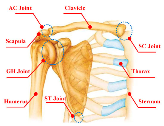
Figure 1.
Anatomy of the shoulder complex (AC: acromioclavicular; SC: sternoclavicular; GH: glenohumeral; ST: scapulothoracic).
Theoretically, all the joints and bones of the shoulder complex are particularly complex [24]. Although some researchers have been looking for an equivalent kinematic structure considering the overall motion characteristics, they do not wholly replicate the shoulder girdle [25]. The mechanistic theory of joint physiology is helpful to understand the shoulder complex kinematics [15].
The GH joint has three revolute DOFs with axes intersecting vertically in the GH joint center and moves with the functional relevance of the shoulder girdle during humeral movements. According to the knowledge of theoretical mechanics, the general motion of a rigid body can be decomposed into translation following any of the base points and rotation relative to the base point. Thus, the shoulder girdle is assumed to be a platform. The mobile reference frame is established on the shoulder girdle, and the origin of the mobile reference frame is G. Relative to the thorax coordinate system O-XYZ (i.e., the coordinate directions are taken from Reference [7]: the x-axis is equal to the frontal axis, and the direction is from the sternum to the GH joint center, the z-axis is equal to the vertical axis, and the direction is upward, y is the cross product of vector z and x, and the coordinate origin is the deepest point of the incisura jugularis [25]), the G point has three translational DOFs. The fixed connection coordinate frame is established on the humerus head, and the origin represented by g is a point on the humerus head coinciding with the GH joint center. Relative to the mobile reference frame, the humerus has three rotational DOFs with axes intersecting vertically at the point g in space. In this way, a generalized GH joint with a floating center (i.e., a 3-DOF spherical joint with a floating center, the center displacement variable of which relative to the thorax coordinate system is coupled with its rotation) is presented, as shown in Figure 2.
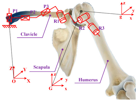
Figure 2.
Mechanism model of the shoulder complex (P1, P2 and P3 denote three prismatic joints, while R1, R2 and R3 denote three revolute joints, respectively).
2.2. Wearable Detection System
According to the mechanism model of the shoulder complex, the center displacement variable relative to the thorax coordinate system is coupled with its rotation. To establish a specific motion coupling relationship between the GH joint center displacement variable quantity relative to the thorax coordinate system and humeral elevation angle, a wearable detection system was designed, which includes the design of the mechanical system, the design of the measurement system and the wearable detection system.
2.2.1. Mechanism System Design
According to the model of the shoulder complex, establishing its kinematic model is equivalent to obtaining the GH joint motion information. The GH joint possesses six DOFs (three rotations and three translations). To completely track the GH joint, a wearable detection mechanism was designed, which possesses three vertical orthogonal translational joints and three rotational joints with axes intersecting vertically in the GH joint center. The detection mechanism includes a horizontal and a vertical tracking mechanism, as shown in Figure 3. The function of the wearable mechanical system is to fully track the motion information of the GH joint in the upper limb accessible workspace.
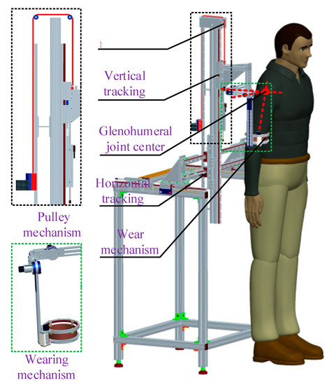
Figure 3.
Wearable detection mechanism.
The horizontal tracking mechanism poses two DOFs, which are mounted on the support plate. It consists of two interconnected guide strip slide mechanisms that are equivalent to prismatic joints and tracks the GH joint displacement variable in the horizontal plane. The vertical tracking mechanism poses one DOF, which is mounted on the horizontal mechanism. It consists of one guide strip slide mechanism and a pulley mechanism. The guide strip slide mechanism tracks the GH joint displacement variable in the vertical axis direction, which has a sufficient range of motion to track the vertical axis direction motion of the GH joint. The pulley mechanism can balance the gravity of the vertical guide strip slide mechanism. The wearing mechanism has three revolute DOFs with axes intersecting vertically at the GH joint center and is mounted to the vertical mechanism. It consists of three revolute joints that are connected to each other and tracks the three-dimensional (3D) rotation of the GH joint.
2.2.2. Measurement System Design
The design of the measurement system includes hardware, software development, and system integration. The hardware mainly includes three displacement sensors (JHQ-DA-50, resolution: 0.001 mm, stroke length: 150 mm, repeatability: 0.002 mm), three incremental encoders (CFZ2124-3600-06-14F, resolution: 3600 pulses per revolution), and an acquisition card (NI-USB-6341). The function of the displacement sensors is to obtain the displacement variable of the GH joint in three dimensions. The incremental encoder obtains the angle motion information of the GH joint during humerus elevation movement. The NI-USB-6341 is used to obtain the signal of the sensors and the incremental encoders, which can be transmitted to the master computer via the USB port. The output of the displacement sensor is analog signal, and the output of the encoder is digital signal. Thus, this detection system needs to simultaneously acquire three channels of analog signals and three channels of digital signals. The human–robot interface is programmed by using LABVIEW.
By connecting the displacement sensor, incremental angle encoder, acquisition card, power supply, and computer, the driver program of the detection system is downloaded. The overall acquisition system is integrated as shown in Figure 4.
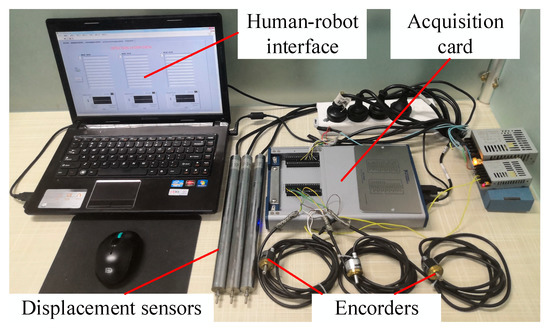
Figure 4.
Diagram of the measurement system.
2.2.3. Wearable Detection System Integration
Combining the data measurement system, the rotation information of the GH joint can be obtained through the connection between the encoder, coupling, and detection mechanism. The translation information of the GH joint can be acquired through the connection between the displacement sensor and the detection mechanism. The data curve in the acquisition process is displayed on the human–robot interface in real time. The wearable detection system integration is shown in Figure 5.
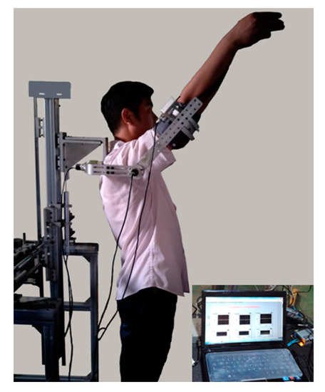
Figure 5.
System integration.
2.3. Experimental Setup
Twelve healthy male subjects were involved in the experiments, with details shown in Table 1. All experiments were approved by the Ethical Committee of Beijing University of Technology, and conformed to the Declaration of Helsinki. The right arm, which is the most commonly used arm, was used during the testing by all participants.

Table 1.
Participant demographics.
Before the experiment, the measurements of the GH joint motion information were recorded with the subjects in the standing position, keeping their arms straight, relaxing the right shoulder such that it hung naturally, with no elbow flexion. To ensure the effectiveness of the experimental data collection, the experiment was conducted on the same day and at the same place. The sampling rate of the detection system was adjusted to be 50 Hz. At the beginning of the experiment, the participant wore the detection mechanism, and the wearing device was adjusted to make the axes of three rotational joints intersect vertically at the GH joint center. The participant performed the internal/external movement several times in the horizontal plane. If the displacement quantity of the horizontal tracking mechanism and vertical tracking mechanism was almost equal to zero, the axes of the three rotational joints of the wearable detection mechanism intersected vertically at the GH joint center [8,21]. Then, the internal/external part of the wearable mechanism was locked because it does not affect the position of the GH joint center [8]. The subjects were asked to raise and lower their humerus in a voluntary fashion several times to ensure the stability of the test data. The first set of experiments was performed to study the motion information of the GH joint in the sagittal and coronal planes. Each participant performed right arm raising and lowering movements for seven cycles in the sagittal and coronal planes respectively, and the wearable detection system presented and recorded the GH joint motion data. The second set of experiments was performed to study the motion coupling relationship between the GH joint center displacement variable quantity and humeral elevation angle in the sagittal and coronal planes. The participants performed elevation of their right arms in the sagittal and coronal planes, and the elevation angle in different planes ranged from 0° to 120°. All the subjects performed the motion three times, and the wearable detection system also presented and recorded the GH joint motion data.
2.4. Post-Processing of the Experimental Data
Considering that the motion data of the GH joint obtained from the wearable detection system is described by using the anatomy method, in which the basic movement of the arm is abduction/adduction α around the sagittal axis, flexion/extension β around the coronal axis, and internal/external γ around the vertical axis, while the daily quantitative description is described in terms of the International Society of Biomechanics (ISB) (i.e., the elevation angle η, the elevation angle θ, and the internal/external angle ψ), there needs to be an equivalent transformation, according to Reference [30], as in Equation (1):
By using Equation (1), the parameters of η, θ, and ψ can be solved. For the first set of experiments, the first cycle and the last cycle were removed from the experimental data results to ensure the stability of the data amplitude and motion period, while for the second set of experiments, the experimental data results were normalized and fitted. However, there may be overfitting and underfitting phenomena during fitting [31,32]. The evaluation indexes are used to select the parameters of the fitting curve. In these indexes, the closer the sum of squares due to error (SSE) and root mean squared error (RMSE) are to zero, the better the model selection, fitting, and data prediction will b. The closer the coefficient of determination (R-Square) and DOF-adjusted coefficient of determination (Adjusted R-Square) are to one, the better the model fits the data. The general criteria are selected, i.e., the R-Square and Adjusted R-Square are greater than 0.995, and the SSE and RMSE are less than 0.005.
3. Results
3.1. GH Joint Motion Information in the Sagittal and Coronal Planes
According to the first experiment, one set of data is described as below: Subject (age 26 years, height 179 cm, weight 82 kg, arm length 551.5 mm) carried out humeral raising and lowering movements for five cycles in the sagittal and coronal planes, and the range of elevation angle was approximately 120°. During natural raising and lowering of the humerus, it is impossible for the humerus movement to be completely guaranteed in the single elevation plane. Actually, the elevation plane angle has a small variability (less than 5°). For the small elevation plane angle changes, the GH joint center displacement variable quantity is almost equal to zero [8,21]. Thus, the single motion elevation plane is assumed.
During the experiments, the movements of the humeral raising and lowering in the sagittal plane and the GH joint center displacement variable relative to the thorax coordinate system in the X-, Y- and Z-directions were observed, which are presented in Figure 6a–d respectively, where the abscissas represent the degree of completion of the five cycles. During the raising and lowering movement of the humerus, the GH joint center displacement variable was large and regular in the X-, Y- and Z-directions, confirming the coupled motion relationship between the GH joint center displacement variable quantity and humeral elevation angle in the sagittal plane. Then, many tests were completed under the same conditions, and the results were consistent.
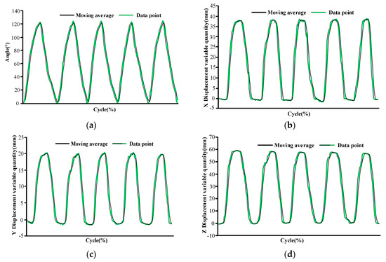
Figure 6.
Diagrams of the glenohumeral (GH) joint motion information relative to the thorax coordinate system during humeral raising and lowering movements of five cycles in the sagittal plane: (a) humeral raising and lowering angle, (b) X-direction of the GH joint displacement variable quantity, (c) Y-direction of the GH joint displacement variable quantity, and (d) Z-direction of the GH joint center displacement variable quantity.
The movements of the humeral raising and lowering in the coronal plane and the GH joint center displacement variable in the X-, Y- and Z-directions are also observed, which are presented in of Figure 7a–d respectively, where the abscissas also represent the degree of completion of the five cycles. During the raising and lowering movements of the humerus, the GH joint center displacement variable was large and regular in the X-, Y- and Z-directions. However, from Figure 6 and Figure 7, we can see that the GH joint displacement variable quantities in the X- and Y-directions of the same subject were different.
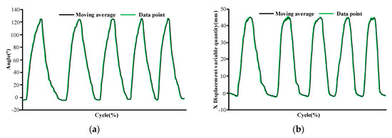
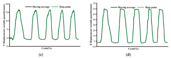
Figure 7.
Diagrams of the GH joint motion information relative to the thorax coordinate system during humeral raising and lowering movements five cycles in the coronal plane: (a) humeral raising and lowering angle, (b) X-direction of the GH joint displacement variable quantity, (c) Y-direction of the GH joint displacement variable quantity, and (d) Z-direction of the GH joint center displacement variable quantity.
3.2. Motion Coupling Relationship in Sagittal and Coronal Planes
According to the second experiment, Figure 8 and Figure 9 show the motion curves (blue lines) for the twelve subjects performing humerus elevation movements in the sagittal and coronal planes, and the elevation angle ranges from 0° to 120°. The movements of the GH joint center displacement variable quantity in the X-, Y- and Z-directions during humeral elevation in the sagittal and coronal planes were observed, which are presented in Figure 8a–c and Figure 9a–c, respectively. Different patterns appear in the two elevation planes relative to the humeral elevation. However, the results are repeated with the same motion trend in the same plane. To summarize the motion coupling relationship, the average data points for the twelve subjects performing humerus elevation movements in the same plane are obtained. To clarify the functional relationship between the GH joint center displacement variable quantity relative to the thorax coordinate system and humeral elevation angle using the average data points, the polynomials of x, y, and z are acquired in different planes according to the guidelines for curve fitting given in Section 2.4. describing the motion coupling relationship between the X-, Y- and Z-magnification ratios.
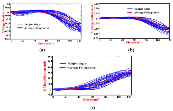
Figure 8.
Diagrams of the magnification ratio of the GH joint center displacement variable quantity relative to the thorax coordinate system during humeral elevation in the sagittal plane: (a) X-magnification ratio and elevation angle, (b) Y-magnification ratio and elevation angle, and (c) Z-magnification ratio and elevation angle.
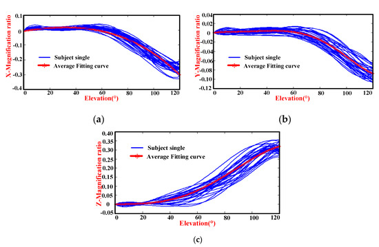
Figure 9.
Diagrams of the magnification ratio of the GH joint center displacement variable quantity relative to the thorax coordinate system during humeral elevation in the coronal plane: (a) X-magnification ratio and elevation angle, (b) Y-magnification ratio and elevation angle, and (c) Z-magnification ratio and elevation angle.
Humeral elevation in the sagittal plane: Observing the mean data, for the polynomial of x, the degree of the polynomial is four. Although the R-Square and Adjusted R-Square are almost equal to one and the SSE and RMSE are almost equal to zero, the fitting curve first rises and then falls in the initial stage, which does not confirm the daily movement rules and may exhibit overfitting [31]. When the degree of the polynomial is three, the values of the SSE and RMSE are 0.0017 and 0.0038, less than 0.005, and the R-Square and Adjusted R-Square are 0.9967 and 0.9966, slightly greater than 0.995, which is consistent with the evaluation indexes of the criteria, and the fitting curve is consistent with the average data. In this way, the degree of the fitting polynomial is chosen to be three. For the polynomial of y, the degree of the polynomial is four. The indexes of the fitting curve are less than the evaluation indexes of the criteria. However, the effect of the fitting curve is not close to the average data. When the degree of the polynomial is five, the effect of the fitting curve is consistent with the average. Thus, the degree of the polynomial selected is five. The polynomials of z show a better fit when the degree of polynomials is four. Then, the evaluation indexes of Xfl, Yfl, and Zfl in appropriate degrees of polynomials, are those listed in Table 2.
Table 2.
Indexes of fitting curve in sagittal and coronal planes.
Humeral elevation in the coronal plane: For the polynomial of x, the degree of the polynomial is three. Although the indexes of the SSE and RMSE are 0.0146 and 0.0112 respectively, which are greater than 0.005, and the R-Square and Adjusted R-Square are 0.9855 and 0.9851 respectively, which are slightly greater than 0.995, the motion trend of the fitting curve is consistent with the average data. When the degree of the polynomial is four, the fitting curve cannot reflect the motion rule of the average data. Although the R-Square is 0.9964, the Adjusted R-Square is 0.9962, the SSE is 0.003639, and the RMSE is 0.005601, which are more in line with the evaluation indexes of the criteria. When the degree of the polynomial is two, the indexes of the fitting curves are not consistent with the evaluation indexes of the criteria, and the fitting effect is not as good when the degree of the polynomial is three and four. Thus, the cubic polynomial is selected. The polynomials of y and z show a better fit when the degree of the polynomials is five and four. The evaluation indexes Xbd, Ybd, and Zbd in appropriate degrees of the polynomials are also shown in Table 2.
Through the above analysis, the motion coupling relationship between the GH joint center displacement variable quantity relative to the thorax coordinate system and the humeral elevation angle in different planes is obtained.
Elevation in sagittal plane: The analytical formulas are presented by the red curves in Figure 8 and named xfl, yfl, and zfl in Equation (2):
Elevation in coronal plane: The analytical formulas are presented by the red curves in Figure 9 and named xbd, ybd, and zbd in Equation (3):
4. Discussion
4.1. Comparison of Collected Data with Result of Klopčar Kinematic Model
4.1.1. Klopčar Kinematic Model
Klopčar used the method of markers (M1–M11) pasted onto the skin of the right shoulder complex, as shown in Figure 10. The angular displacement data corresponding to the joints of the shoulder complex when the upper arm is elevated in the 0°, 45°, 90°, and 135° planes were obtained. The measurements were combined to cover the entire reachable domain of the humerus in the above-defined planes [8]. Through the analysis and integration of the data measured in the experiment, the coupling relationship between the movements of the shoulder girdle and humeral elevation angle was obtained. Therefore, the angle ϕed of elevation/depression and the ϕpr of protraction/retraction were calculated according to Equations (4) and (5) during humeral elevation, respectively.
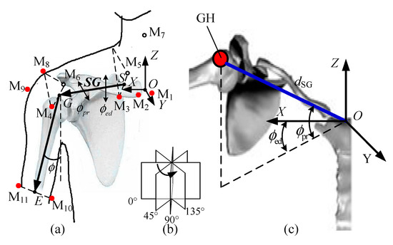
Figure 10.
(a) Reference points on the shoulder complex and the center of the GH joint in global coordinate frame. (b) four anatomical planes. (c) calculated position of the GH joint center in the global coordinate system.
The length of the shoulder girdle dSG can be expressed as in Equation (6):
where ϕ is the elevation angle and d0 is the shoulder girdle from S to G when the arm of the subject is hanging naturally.
For the Klopčar kinematic model, the origin of the global coordinate system is the crossing of an axis (medial and lateral) through the GH joint center and an axis (anterior and posterior) through the thorax. The calculated reference point is the center of the M3 and M5 markers, which is not clear, leading to difficult estimates. However, the distance from the center of the sternum to point G is three-quarters of the initial distance from that, as presented in Reference [21]. Considering that the coordinate frames are different, we unify the starting point at the GH joint initial coordinate frame. Thus, the Klopčar kinematic model is transformed into Equation (7) based on formulas from Equations (4) to (6).
4.1.2. Comparison of Collected Data in the Sagittal and Coronal Planes
According to Equation (7), x(ϕ), y(ϕ), and z(ϕ) are zero when the elevation angle is equal to zero. For the unity of the results, the constant terms of xfl, yfl, zfl, xbd, ybd, and zbd of the GH joint center displacement variable quantity are ignored, which are named xfli, yfli, zfli, xbdi, ybdi, and zbdi. Thus, the results are presented in Figure 11a–c and Figure 12a–c, respectively. For further comparison, the displacement variable quantities d(ϕ), x(ϕ), y(ϕ), and z(ϕ) of the Klopčar kinematic model are also added to Figure 11 and Figure 12, which are obtained based on Equation (7).
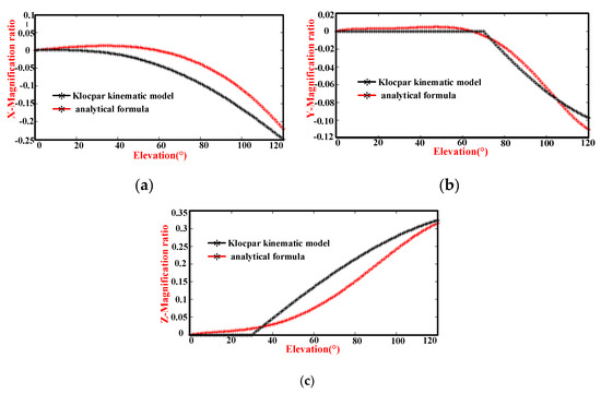
Figure 11.
Comparison of the magnification ratio of the GH joint center displacement variable quantity relative to the thorax coordinate system during humeral elevation in the sagittal plane and the Klopčar kinematic model: (a) translational displacement variable quantities xfli and x(Φ), (b) translational displacement variable quantities yfli and y(Φ), and (c) translational displacement variable quantities zfli and z(Φ).
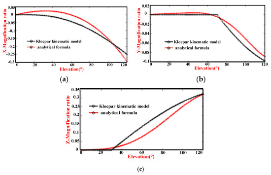
Figure 12.
Comparison of the magnification ratio of the GH joint center displacement variable quantity relative to the thorax coordinate system during humeral elevation in the coronal plane and the Klopčar kinematic model: (a) translational displacement variable quantity xbdi and x(Φ), (b) translational displacement variable quantity ybdi and y(Φ), and (c) translational displacement variable quantity zbdi and z(Φ).
In Figure 11a, the displacement variable quantity xfli changes slightly with the angle ϕ, from 0° to 60°. Then, the curve assumes a convex shape between 60° and 120°. The GH joint center displacement variable quantity x(ϕ) along the x-axis moves slightly with an angle ϕ, from 0° to 40°. Then, the curve also assumes a convex shape between 40° and 120°. Observing the two curves, the trend is basically the same except for the magnitude.
In Figure 11b, the displacement variable quantity yfli changes slightly with the angle ϕ from 0° to 55°, and the gradient of the curve decreases from 55° to 110°, the change in which is large. Then, the gradient of the curve rises slightly with the angle ϕ, from 110° to 120°. The GH center displacement variable quantity y(ϕ) along the y-axis stays in the same position as the angle ϕ changes from 0° to 70°. The gradient of the curve decreases from 70° to 110°, the change in which is very evident. From 110° to 120°, the gradient of the curve does not change significantly. The curve yfli is smoother than that of y(ϕ). The motion pattern in the middle position and at the end position is slightly different. Given that y(ϕ) is the sum of the four elevation planes, the reasonable analysis results of yfli are acceptable.
In Figure 11c, the displacement variable quantity zfli changes steadily with the angle ϕ, from 0° to 30°. However, the change is very small. The increases in displacement variable quantity zfli are first large and then small as the angle ϕ changes from 30° to 120°. The displacement variable quantity z(ϕ) along the z-axis does not move with angle ϕ values from 0° to 30°, which matches zfli. When the elevation is from 30° to 120°, the data increment is larger than zfli. Considering the experimental data obtained by our detection system, the motion of zfli is somewhat delayed from 30° to 120°. However, the displacements z(ϕ) and zfl are almost the same at an elevation of 120°.
In Figure 12a, the displacement variable quantity xbdi changes slightly with the angle ϕ, from 0° to 40°. Then, as the angle increases from 40° to 120°, the gradient decreases. The GH joint center displacement variable quantity x(ϕ) along the x-axis moves slightly with the angle ϕ from 0° to 40°. The gradient and angle present a negative correlation from 40° to 120°. The magnitude of xbdi is greater than that of x(ϕ). Because the magnitude of xfli is less than that of x(ϕ), the movement law of xbdi is reasonable.
In Figure 12b, the displacement variable quantity ybdi changes slightly in the initial stage, and the gradient of the curve decreases in the middle phase, the change in which is large. Then, the gradient of the curve rises slightly in the end. The GH center displacement variable quantity y(ϕ) along the y-axis stays in the same position as the angle ϕ changes from 0° to 70°. The gradient of the curve decreases from 70° to 110°, the change in which is very evident. From 110° to 120°, the gradient of the curve does not have considerable change. Although the two curves differ in amplitude, the result is acceptable.
In Figure 12c, the displacement variable quantity zbdi changes steadily with the angle ϕ, from 0° to 20°. However, the change is very small. The increases in displacement variable quantity zbdi are first large and then small as the angle ϕ changes from 20° to 120°. The displacement variable quantity z(ϕ) along the z-axis does not move with angle ϕ values from 0° to 30°, which basically matches zbdi. When the elevation is from 30° to 120°, the data increment is also larger than zbdi. Although the motion of zbdi is somewhat delayed from 30° to 120°, the trend is basically the same.
Based on the above analysis of Figure 11 and Figure 12, although the collected data in the sagittal and coronal planes were different from the comparative analysis of the Klopčar kinematic model, the trends are almost the same. The Klopčar kinematic model was the result of the synthesis of four planes, and this study is considered only at a single elevation plane and takes into account different experimental processing methods. This result is sufficient for daily exercise and the design of rehabilitation training equipment.
4.2. Comparison of the Motion Coupling Characteristics in the Sagittal and Coronal Planes
Although the constant term of the analytic equation is not equal to zero, the coefficient is small, and we assume that the GH joint displacement variable quantity is zero at the initial time. Therefore, the premise is that the GH joint center displacement variable quantity in different planes is considered to be zero when the elevation angle is zero. Based on the above conditions, xbdi, ybdi, and zbdi of the GH joint center displacement variable quantity are shown in Figure 13a–c, respectively. For further comparison, the displacement variable quantities xfli, yfli, and zfli are added.
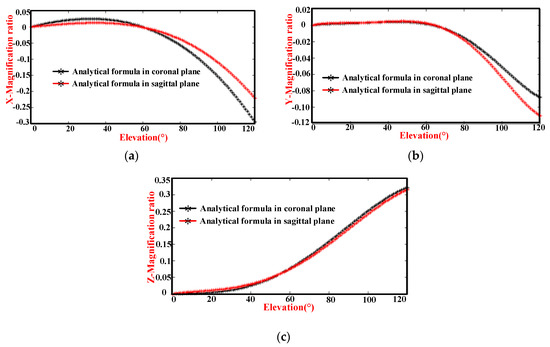
Figure 13.
Comparison of the magnification ratio of the GH joint center displacement variable quantity relative to the thorax coordinate system during humeral elevation in the coronal and sagittal planes: (a) X-direction magnification ratio and humeral elevation angle, (b) Y-direction magnification ratio and humeral elevation angle, and (c) Z-direction magnification ratio and humeral elevation angle.
The changes in the X-direction are shown in Figure 13a. During humeral elevation in the coronal plane, the slope of the curve is relatively small in the initial stage, and then increases. When humeral elevation is in the sagittal plane, the slope is small in the initial stage, and then the slope decreases. They intersect in the middle. After that, they basically follow the same slope. Although the movement trends are also the same, the magnitude of the motion is different. The difference in the magnification ratio is 0.074 at the 120° elevation angle.
The changes in the Y-direction are shown in Figure 13b. The slope of the curve during humeral elevation in the coronal plane is essentially unchanged in the initial stage and then gradually increases. The slope of the humeral elevation in the sagittal plane is also the same in the initial stage. Subsequently, this slope gradually and rapidly decreases. In the last stage, they gradually maintain the same slope. However, the motion range in the coronal plane is less than that in the sagittal plane. The difference in the magnification ratio is 0.023 at an elevation angle of 120°.
The changes in the Z-direction are shown in Figure 13c. The humeral elevation in the coronal plane, the magnification ratio, and the elevation angle are positively correlated during humeral elevation from 0° to 120°, except for a weak correlation in the initial and last stages. In the sagittal plane, the magnification ratio is also the same as that in the coronal plane of humeral elevation.
Through the analysis of Figure 13 and because the influences of the detection accuracy and measurement error under the same experimental conditions are similar, their motion trends are not the same, which confirms the different motion characteristics in different planes.
5. Conclusions
Due to the complex coupled motion of the shoulder mechanism, the design of the guiding movement rules of rehabilitation robots generally lacks specific motion coupling information between the GH joint center and humeral elevation angle to describe the shoulder complex. To obtain the specific motion coupling information, the first step is to establish a mechanism model of the shoulder complex. However, to model the movements of the shoulder complex, the joint coupling motion relationship between the GH joint and the shoulder girdle during humeral elevation as well as their differences during humeral elevation in different planes should be considered.
In this work, considering the whole coupled motion of the shoulder complex for a given pointing position, a mechanism model of the shoulder complex, which is a generalized GH joint with a floating center, was presented. The GH joint center displacement variable quantity relative to the thorax coordinate system is equal to the overall motion of the shoulder girdle, and the coupled motion can clearly describe the characteristics of the shoulder girdle and GH joint. Then, a wearable detection system was designed, and the experiment was set up with data processed. This study also established a kinematic model of the shoulder complex in the sagittal and coronal planes and evaluated the differences in GH joint motion during humeral elevation in the sagittal and coronal planes.
The experimental results presenting the GH joint motion information during humerus raising and lowering movements in the sagittal and coronal planes were presented. Going a step further, the motion coupling relationship between the GH joint center displacement variable quantity and humeral elevation angle in the sagittal plane and coronal planes was obtained. This is also consistent with the results of other researchers [21,25]. However, it should be highlighted that due to the effect of the deviation of the skin from the bone target during movement of the arm, wear deviation, and the GH joint being modeled as a simplified spherical joint, the kinematic model can only be applied to provide basic data for the design of the shoulder exoskeleton mechanism, shoulder function simulation, and ergonomics, while it cannot be used in joint replacement, prosthesis design, and other areas that need accurate kinematic information [22]. The exact coupled motion information between the GH joint and shoulder girdle using a pin inserted into the sternum, clavicle, scapula, and humerus will be addressed in our future work.
Nevertheless, this study provides a new method to obtain the kinematic model of the shoulder complex obtained from a wearable detection system in an accessible workspace, and the results provide basic data for the design of the shoulder exoskeleton mechanism and have practical significance for the daily human movement science.
Author Contributions
Formal analysis, C.Z.; Funding acquisition, J.L. and M.D.; Methodology, J.L., C.Z. and M.D.; Validation, J.L. and Q.C.; Writing—original draft, C.Z.; Writing—review and editing, M.D. and Q.C. All authors have read and agreed to the published version of the manuscript.
Funding
This research was funded in part by the National Natural Science Foundation of China, grant numbers 51675008 and 61903011, in part by the Beijing Natural Science Foundation, grant numbers 3171001, 17L20019, and 3204036, and in part by Beijing Postdoctoral Research Foundation, grant number Q6001002201901.
Acknowledgments
The authors would like to acknowledge the National Research Center for Rehabilitation Technical Aids, Beijing, China, for the meaningful guidance on the development of the kinematic model.
Conflicts of Interest
The authors declare no conflict of interest.
References
- Jackson, M.; Michaud, B.; Tétreault, P.; Begon, M. Improvements in measuring shoulder joint kinematics. J. Biomech. 2012, 45, 2180–2183. [Google Scholar] [CrossRef] [PubMed]
- Mao, A.; Ma, X.; He, Y.; Luo, J. Highly portable, sensor-based system for human fall monitoring. Sensors 2017, 17, 2096. [Google Scholar] [CrossRef] [PubMed]
- Nam, H.S.; Lee, W.H.; Gil Seo, H.; Kim, Y.J.; Bang, M.S.; Kim, S. Inertial measurement unit based upper extremity motion characterization for action research arm test and activities of daily living. Sensors 2019, 19, 1782. [Google Scholar] [CrossRef]
- Feng, X.; Yang, J.; Karim, A.M. Survey of biomechanical models for human shoulder complex. Soc. Automot. Eng. Tech. 2008, 1, 1871. [Google Scholar]
- Tondu, B. Estimating shoulder-complex mobility. Appl. Bionics Biomech. 2007, 4, 19–29. [Google Scholar] [CrossRef]
- Li, J.; Zhang, Z.; Tao, C.; Ji, R. A number synthesis method of the self-adapting upper-limb rehabilitation exoskeletons. Int. J. Adv. Robot. Syst. 2017, 14, 1–14. [Google Scholar] [CrossRef]
- Hingtgen, B.; McGuire, J.R.; Wang, M.; Harris, G.F. An upper extremity kinematic model for evaluation of hemiparetic stroke. J. Biomech. 2006, 39, 681–688. [Google Scholar] [CrossRef]
- Klopčar, N.; Lenarčič, J. Bilateral and unilateral shoulder girdle kinematics during humeral elevation. Clin. Biomech. 2006, 21, 20–26. [Google Scholar] [CrossRef]
- Dvir, Z.; Berme, N. The shoulder complex in elevation of the arm: A mechanism approach. J. Biomech. 1978, 11, 219–225. [Google Scholar] [CrossRef]
- Tobias, N.; Marco, G.; Robert, R. ARMin III-Arm Therapy Exoskeleton with an Ergonomic Shoulder Actuation. Appl. Bionics Biomech. 2009, 6, 127–142. [Google Scholar]
- Lenarcic, J.; Umek, A. Simple model of human arm reachable workspace. IEEE Trans. Syst. Man Cybern. Syst. 1994, 24, 1239–1246. [Google Scholar] [CrossRef]
- Yang, J.; Abdel-Malek, K.; Nebel, K. Reach envelope of a 9-degree-of-freedom model. Int. J. Robot. Autom. 2005, 20, 240–259. [Google Scholar]
- Lenarčič, J.; Stanisic, M. A humanoid shoulder complex and the humeral pointing kinematics. IEEE Trans. Robot. Autom. 2003, 19, 499–506. [Google Scholar] [CrossRef]
- Yang, J.J.; Feng, X.Y. Determining the three-dimensional relation between the skeletal elements of the human shoulder complex. J. Biomech. 2009, 42, 1762–1767. [Google Scholar] [CrossRef] [PubMed]
- Tondu, B. Modelling of the shoulder complex and application the design of upper extremities for humanoid robots. In Proceedings of the 2005 5th IEEE-RAS International Conference on Humanoid Robots, Tsukuba, Japan, 5–7 December 2005; pp. 313–320. [Google Scholar]
- Maurel, W.; Thalmann, D. A Case Study on Human Upper Limb Modelling for Dynamic Simulation. Comput. Methods Biomech. Biomed. Eng. 1999, 2, 65–82. [Google Scholar] [CrossRef] [PubMed]
- Berthonnaud, E.; Herzberg, G.; Zhao, K.D.; An, K.N.; Dimnet, J. Three-dimensional in vivo displacements of the shoulder complex from biplanar radiography. Surg. Radiol. Anat. 2005, 27, 214–222. [Google Scholar] [CrossRef]
- Lenarcic, J.; Staniaie, M.M. Kinematic design of a humanoid robotic shoulder complex. In Proceedings of the IEEE International Conference on Robotics and Automation, San Francisco, CA, USA, 24–28 April 2000; pp. 27–32. [Google Scholar]
- Kirsch, R.F.; Acosta, A.M. Model-based development of neuroprostheses for restoring proximal arm function. J. Rehabil. Res. Dev. 2001, 38, 619–626. [Google Scholar]
- Van Der Helm, F. A finite element musculoskeletal model of the shoulder mechanism. J. Biomech. 1994, 27, 551–569. [Google Scholar] [CrossRef]
- Newkir, J.T.; Tomsic, M.; Crowell, C.R. Measurement and quantification of the human shoulder girdle motion. Appl. Bionics Biomech. 2013, 10, 159–173. [Google Scholar] [CrossRef]
- Braman, J.; Engel, S.C.; Laprade, R.F.; Ludewig, P.M. In vivo Assessment of Scapulohumeral rhythm during unconstrained overhead reaching in asymptomatic subjects. J. Shoulder Elbow Surg. 2011, 18, 960–967. [Google Scholar] [CrossRef]
- Högfors, C.; Peterson, B.; Sigholm, G.; Herberts, P. Biomechanical model of the human shoulder joint-II. The shoulder rhythm. J. Biomech. 1991, 24, 699–709. [Google Scholar] [CrossRef]
- Sholukha, V.; Jan, S.V.S. Combined motions of the shoulder joint complex for model-based simulation: Modeling of the shoulder rhythm (ShRm). In 3d Multiscale Physiological Human; Spring: London, UK, 2014; pp. 205–232. [Google Scholar]
- Yan, H.; Yang, C.; Zhang, Y.; Wang, Y. Design and validation of a compatible 3-degree-of-freedom shoulder exoskeleton with an adaptive center of rotation. J. Appl. Mech. Trans. ASME 2014, 136, 071006. [Google Scholar] [CrossRef]
- Scano, A.; Molteni, F.; Tosatti, L.M. Low-cost tracking systems allow fine biomechanical evaluation of upper-limb daily-life gestures in healthy people and post-stroke patients. Sensors 2019, 19, 1224. [Google Scholar] [CrossRef] [PubMed]
- Lenarčič, J.; Klopčar, N. Positional kinematics of humanoid arms. Robotica 2006, 24, 105–112. [Google Scholar] [CrossRef]
- Laitenberger, M.; Raison, M.; Périé, D.; Begon, M. Refinement of the upper limb joint kinematics and dynamics using a subject-specific closed-loop forearm model. Multibody Syst. Dyn. 2014, 33, 1–26. [Google Scholar] [CrossRef]
- Schnorenberg, A.J.; Slavens, B.A.; Wang, M.; Vogel, L.C.; Smith, P.A.; Harris, G.F. Biomechanical model for evaluation of pediatric upper extremity joint dynamics during wheelchair mobility. J. Biomech. 2014, 47, 269–276. [Google Scholar] [CrossRef] [PubMed]
- Rab, G.T. Shoulder motion description: The ISB and Globe methods are identical. Gait Posture 2008, 27, 702–705. [Google Scholar] [CrossRef]
- Hawkins, D.M. The problem of overfitting. J. Chem. Inf. Comput. Sci. 2004, 44, 1–12. [Google Scholar] [CrossRef]
- Van Der Aalst, W.M.P.; Rubin, V.; Verbeek, E.; Van Dongen, B.F.; Kindler, E.; Günther, C.W.; Van Dongen, B. Process mining: A two-step approach to balance between underfitting and overfitting. Softw. Syst. Modeling 2010, 9, 87–111. [Google Scholar] [CrossRef]
© 2020 by the authors. Licensee MDPI, Basel, Switzerland. This article is an open access article distributed under the terms and conditions of the Creative Commons Attribution (CC BY) license (http://creativecommons.org/licenses/by/4.0/).