Analysis of Undrained Seismic Behavior of Shallow Tunnels in Soft Clay Using Nonlinear Kinematic Hardening Model

Abstract

In this study, a soil–tunnel model for clay under earthquake loading is analyzed, using finite element methods and a kinematic hardening model with the Von Mises failure criterion. The results are compared with those from the linear elastic–perfectly plastic Mohr–Coulomb model. The latter model does not consider the stiffness degradation caused by imposing cyclic loading and unloading to the soil, whereas the kinematic hardening model can simulate this stiffness degradation. The parameters of the kinematic hardening model are calibrated based on the results of experimental cyclic tests and finite element simulation. Here, two methods—one using data from cyclic shear tests, and the other a new method using undrained cyclic triaxial tests—are used to calibrate the parameters. The parameters investigated are the peak ground acceleration (PGA), tunnel lining thickness, tunnel shape, and tunnel embedment depth, all of which have an effect on the resistance of the shallow tunnel to the stresses and deformations caused by the surrounding clay soils. The results show that unlike traditional models, the nonlinear kinematic hardening model can predict the response reasonably well, and it is able to create the hysteresis loops and consider the soil stiffness degradation under the seismic loads.

1. Introduction

With the growing populations in metropolitan cities around the world, underground urban infrastructure development has become a major focus. If these underground structures are constructed in earthquake areas, their dynamic response to seismic loads must be determined in order to reduce economic damage and threats to human safety. In contrast to overground structures where design is based on the fact that earthquakes manifest as inertial forces, in underground structures such as tunnels, which have a significant degree of containment, design and analysis are based on the assumption that earthquakes primarily deform the soil structure. Previously, engineers believed that earthquakes caused less destruction of underground structures than surface structures, but the earthquakes of the 1990s caused serious damage to tunnels, forcing a re-appraisal of this view. In recent years, there have been numerous examples in different countries of earthquakes causing extensive damage to underground structures (e.g., the Kobe earthquake, 1995; Taiwan, 1999) [1,2,3,4,5,6,7], which indicates that it is crucial for studies to be made of the seismic behavior of tunnels.

As earthquake waves are usually amplified by passing through different layers of soil (e.g., clay or sand) [8], the surrounding soil can affect the performance of structures such as tunnels [9,10]. Previous studies have shown that tunnels located in clay soils are more likely to be damaged by earthquakes than those constructed in sandy soils [11,12,13,14]. However, there are fewer studies on the seismic behavior of tunnels located in soft soils than in sandy soils. Different approaches such as numerical [15,16,17] and experimental methods [18,19] are used to investigate the seismic behavior of tunnels in terms of the interactions between soil and tunnel.

Using numerical methods to investigate the dynamic behavior of tunnels requires a suitable constitutive model for the materials involved. In recent years, researchers have used numerical methods with different constitutive models to study the seismic behavior of tunnels. Kontoe et al. [5] used a modified Cam-clay constitutive model to investigate the dynamic response of tunnels during the 1999 Duzce earthquake in Turkey. Their results showed that this constitutive model was not suitable for simulating the seismic behavior of a tunnel during strong earthquakes. Debiasi et al. [20] investigated the dynamic response of shallow rectangular tunnels to earthquake loads. Their analysis was conducted mainly with pseudo-static finite element analyses, and it showed that these structures are strongly affected by nonlinear frictional effects at the soil–structure interface. Patil et al. [21] conducted a numerical study on the behavior of tunnels under seismic loads using PLAXIS2D software and a modified Cam-Clay model to model the soil medium. The results of the nonlinear plane strain analysis of the soil–tunnel system showed that the earthquake frequency affected the maximum and residual dynamic Earth pressure around the tunnel. Lei Zhang and Yong Liu [13] studied the seismic behavior of tunnel in clays under earthquake loads, with consideration of the hysteresis–hyperbolic constitutive model for soil. Their results suggested that randomness in the small-strain shear modulus of clay can significantly influence the shear force, the seismic responses of bending moments, and the lateral deformation of tunnels. Xiaohua Bao et al. [22] studied the dynamic behavior of a metro subway tunnel under earthquake loads, using a cyclic elastoplastic constitutive model for foundation soils so as to obtain acceptable results, and they also studied various parameters that affect the seismic behavior of a tunnel. Their work showed that the acceleration response decreased at different depths in the model due to the phenomenon of liquefaction. Moreover, the increase in the amplitude of vertical acceleration increased the liquefaction area.

Soil response to loads is strain-dependent. The behavior of soil under very small strains (γ < 10⁻⁵) is linear elastic, but under higher strains, its behavior is nonlinear. Therefore, it is essential to select an appropriate constitutive model to consider nonlinear strain-dependent stiffness under different loads in a numerical analysis. Although many scholars have used numerical simulation methods to investigate the seismic behavior of soil–structure interactions (e.g., soil–tunnel interactions), an appropriate and more advanced constructive model would better predict the actual behavior of soil under earthquake forces. The use of some constitutive models such as Prevost’s multi-yield model and the intergranular strain anisotropy model (ISA) requires complex calibration to determine their various parameters, which decreases their utility in research [23]. However, isotropic/kinematic plastic hardening models, comprising isotropic and kinematic hardening components, accurately predict soil behavior under dynamic loads.

The main theories on the hardening of soil are isotropic hardening, the linear and nonlinear kinematic hardening model of Armstrong–Frederick [24], and the nonlinear kinematic hardening model of Chaboche [25]. Isotropic hardening occurs when a yield surface is uniformly large, whereas kinematic hardening occurs when the center of the yield surface moves in stress space without the initial yield surface size changing, which is known as the Bauschinger effect [26,27]. Finally, if the size and center of the yield surface change simultaneously, this is denoted as combined hardening. As soils exhibit anisotropic kinematic hardening behavior, isotropic models are not suitable for studying soil behavior under seismic loads. Thus, we use a nonlinear kinematic hardening model in this study, which is a simplified version of the combined isotropic/kinematic hardening model generated by assuming that the size of the yield surface is constant [28].

In this study, a kinematic hardening constitutive model based on the Von Mises failure criterion is been used to investigate the seismic behavior of tunnels in clay soil. In some constitutive models, such as the Cam-clay and modified Cam-clay models used in previous studies, the yield surface is presumed to expand with increasing loading level. This means that when the soil experiences a larger stress surface under dynamic loading, the behavior of the materials will be quite elastic at lower loading levels until the soil sample again experiences stresses greater than the previous yield stress. Therefore, these constitutive models cannot model the Bauschinger effect nor determine the hysteresis loops that exist under cyclic loading, which means that these models cannot predict the actual behavior of soil under kinematic loads, such as seismic loads. However, a kinematic hardening model can be used as an advanced model for the simulation of soil behavior, thereby overcoming these problems. Here, the phenomenon of liquefaction has not been considered and there is no generation of pore pressures. The phenomenon of cyclical degradation and degradation soil stiffness are due to soil structure.

We investigate the factors affecting the behavior of tunnels in clay under earthquake load, including the earthquake intensity, tunnel shape, embedment depth, and lining thickness. Then, we compare our results with the results of Patila et al. [29]. The earthquake used in this study is a 1D earthquake with a dominant frequency of 1 Hz, and the 0.4 g and 0.83 g maximum accelerations that occurred in 1995 in Kobe, Japan. A viscous spring boundary is used around the soil model to prevent the return of earthquake waves into the model, thus ensuring that actual results are obtained.

2. Constitutive Model and Calibration

2.1. Constitutive Model

The function of yield surface, considering the Von-Mises criterion, is defined by Equation (1) [30]:

$$F=f\left({\sigma }_{ij},{\alpha }_{ij}\right)=\sqrt{3J_2\left({\sigma }_{ij}-{\alpha }_{ij}\right)}-{\sigma }_0$$

(1)

where ${\sigma }_o$ is the initial size of the yield surface under zero plastic strain, i.e., at the elastic stress limit, ${\alpha }_{ij}$ is the back stress that refers to the center position of the yield surface, and $J_2\left({\sigma }_{ij}\right)$ is the second deviatoric stress invariant, given by Equation (2):

$$J_2\left({\sigma }_{ij}-{\alpha }_{ij}\right)=\frac{1}{2}\left(S_{mn}-t_{mn}\right).\left(S_{mn}-t_{mn}\right)$$

(2)

where ${\sigma }_{ij}$ and ${\alpha }_{ij}$ are the stress and back stress tensor, respectively, and $S_{mn}$ and $t_{mn}$ are the stress and back stress deviatoric tensor, respectively.

At an infinitely large plastic strain, when ${\sigma }_{ij}$ approaches the effective maximum yield stress (${\sigma }_y$) (Equation (3)), the back stress tensor (${\alpha }_{ij}$) is given by Equation (4), as follows:

$${\sigma }_y=\sqrt{J_2\left({\sigma }_{ij}\right)}$$

(3)

$${\alpha }_{ij}={\alpha }_s=\sqrt{\frac{1}{2}\left(t_{mn}.t_{mn}\right)}.$$

(4)

The important aspect of the kinematic hardening model is the back stress evolution law, which describes the translation of the yield surface in the stress space. The kinematic hardening model consists of two parts—a purely kinematic term and a relaxation term—and can be written as (Equation (5)):

$$d{\alpha }_{ij}=C\frac{1}{{\sigma }_o}\left({\sigma }_{ij}-{\alpha }_{ij}\right)d{\epsilon }^{pl}-{\gamma }_o{\alpha }_{ij}d{\epsilon }_{pl}$$

(5)

where $C$ and ${\gamma }_o$ are material parameters, $d{\epsilon }^{pl}$ is the plastic strain rate tensor, and $d{\epsilon }_{pl}$ is the equivalent plastic strain rate. In relaxation terms, the back stress is related to the equivalent plastic strain and the linear kinematic model is transformed to the nonlinear kinematic model. The plastic flow rule associated with the yield function is as follows (Equation (6)) [30]:

$$d{\epsilon }^{pl}=d\lambda \frac{\partial F}{\partial {\sigma }_{ij}}$$

(6)

where the constant $d\lambda$ is defined as $d\lambda =d{\epsilon }_{pl}$. The detailed expression can be found in Appendix A.

Parameter ${\sigma }_0$ represents the initial size of the yield surface at zero plastic strain and controls the onset of nonlinear soil behavior; it is defined as the fraction ($\lambda$) of the (${\sigma }_y$) effective maximum yield stress at large plastic strain. Decreasing this ratio improves the model nonlinearity, but if it is too small, the model will be non-economic. In contrast, an excessive increase in this quantity has a negative effect on the model that leads to unrealistic results. In the 1D condition, it is given by Equation (7):

$${\sigma }_0=\lambda {\sigma }_y$$

(7)

where $\lambda$ is the material constant.

The evolution equation of kinematic hardening can be integrated to give Equation (8):

$$\alpha =\raisebox{1ex}{$C$}\!\left/ \!\raisebox{-1ex}{${\gamma }_o$}\right.\left[1-exp\left(-{\gamma }_o{\epsilon }_{pl}\right)\right]$$

(8)

where $\alpha$ is the back stress, ${\epsilon }_{pl}$ is the equivalent plastic strain, $C$ is the initial kinematic hardening modulus ($C=E=2\left(1+\nu \right)G_0$) that defines the maximum translation of the yield surface, and ${\gamma }_o$ defines the rate decrease of the kinematic hardening modulus. Parameter $C$ can be derived by differentiating Equation (8) to give Equation (9):

$$\frac{\partial \alpha }{\partial {\epsilon }_{pl}}{|}_{{\epsilon }_{pl}\to 0} C=E.$$

(9)

The occurrence of displacement of the yield surface and the creation of back stress (${\alpha }_{ij}$) in cyclic loading can be understood by considering the kinematic hardening model. At infinite large plastic strain (when ${\sigma }_{ij}$ approaches ${\sigma }_y$), the back stress (${\alpha }_{ij}$) is equal to ${\alpha }_s=\raisebox{1ex}{$C$}\!\left/ \!\raisebox{-1ex}{${\gamma }_o$}\right.$ and (${\sigma }_{ij}-{\alpha }_{ij}$) tends to ${\sigma }_0$ (see Figure 1), which means that Equation (5) tends to zero. 1 illustrates the parameters and notation used in the equations.

2.2. Calibration of Parameters and Model Validation

The parameters of constitutive models of soils are often obtained by comparing experimental results and numerical simulations using finite elements at the element test level [31]. In this study, experimental data from an undrained cyclic triaxial test are used to calibrate the parameter $C$, and two methods for calibrating the parameters $\lambda$, ${\gamma }_o$, and ${\sigma }_0$ are presented. First, the curve of the undrained Young’s modulus versus axial strain is drawn using the results obtained from the cyclic triaxial test and numerical simulations of the test to obtain the $\lambda$ parameter. Second, data from a cyclic shear test and Ishibashi and Zhang’s equations [32] are used.

The values of the parameters such as the undrained shear strength ($S_u$), maximum shear modulus ($G_{max}$) or shear wave velocity ($V_s$), and curve of the undrained Young’s modulus versus axial strain ($E_u$ Vs. ${\epsilon }_1$) are required to calibrate the parameters. A series of undrained cyclic triaxial and monotonic tests of kaolin clay were conducted by Wichtmann [33] in both stress and strain control modes and under different level stress amplitudes.

In this study, the results of monotonic and cyclic tests under the stress control condition with an effective mean pressure of 200 kPa are used to calibrate the constitutive model parameters. The process mentioned above, by which the parameters of the model are calibrated, is fully described below.

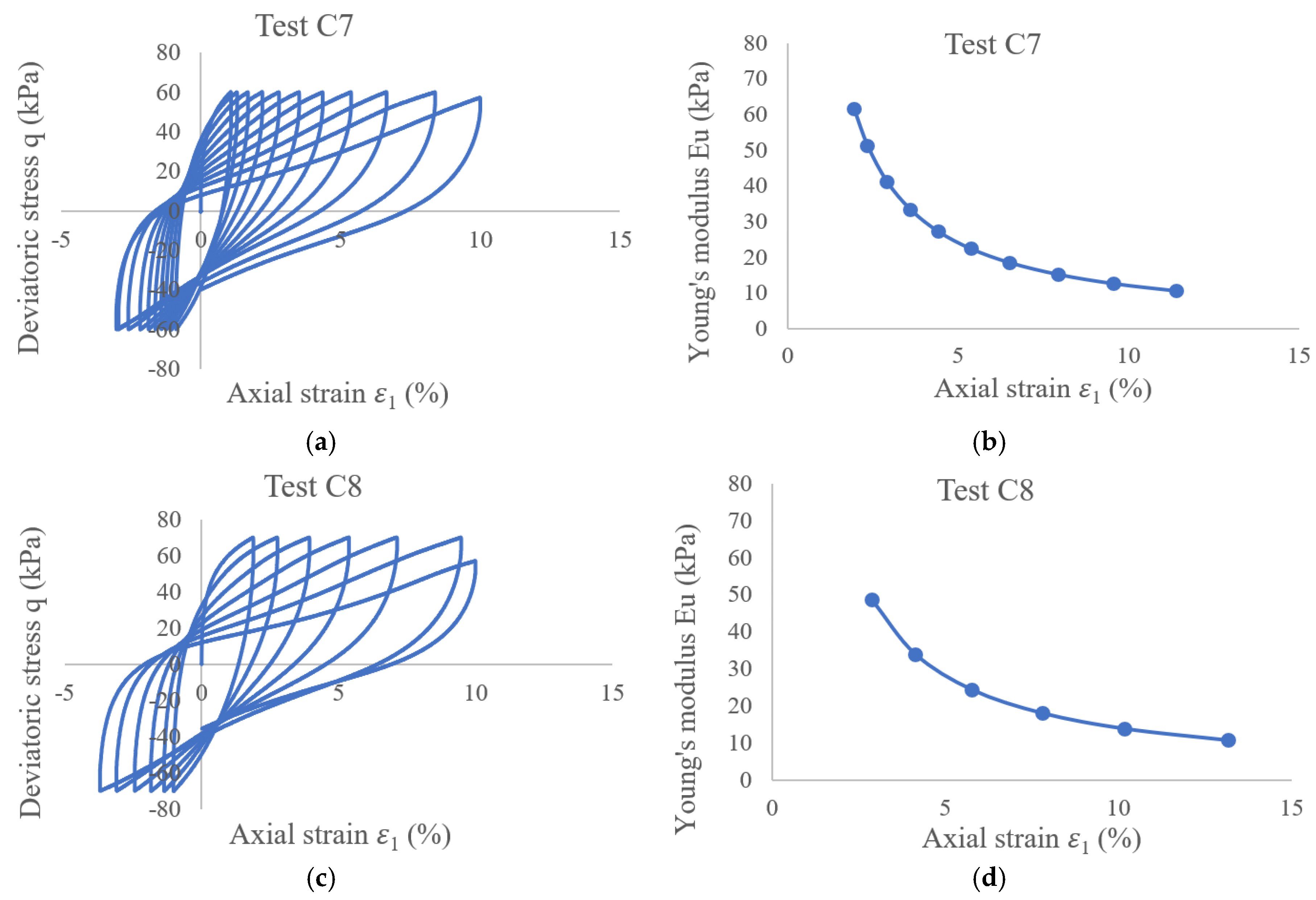
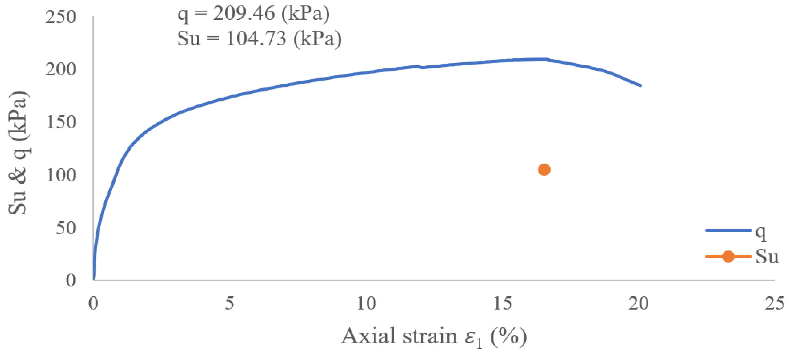
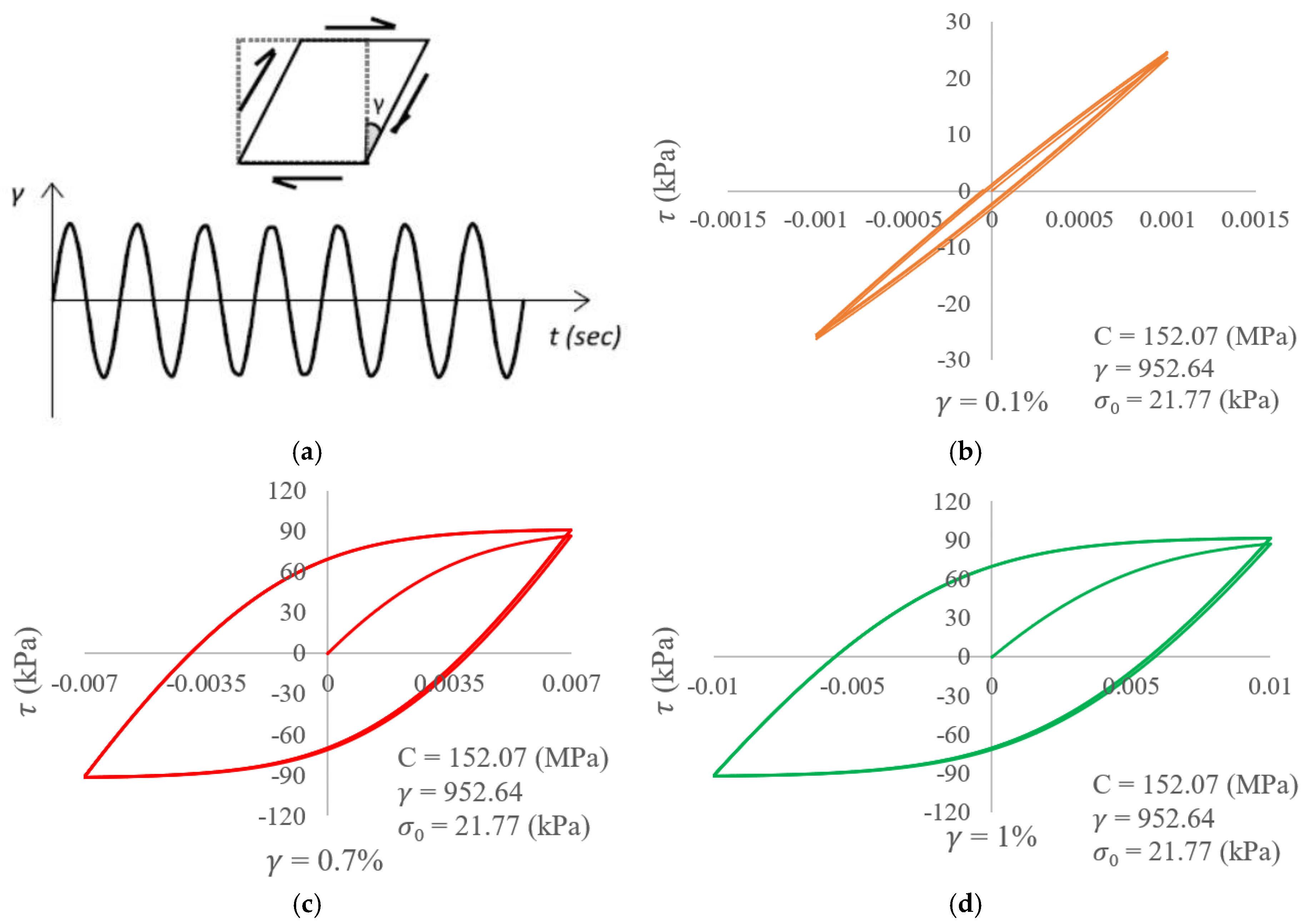
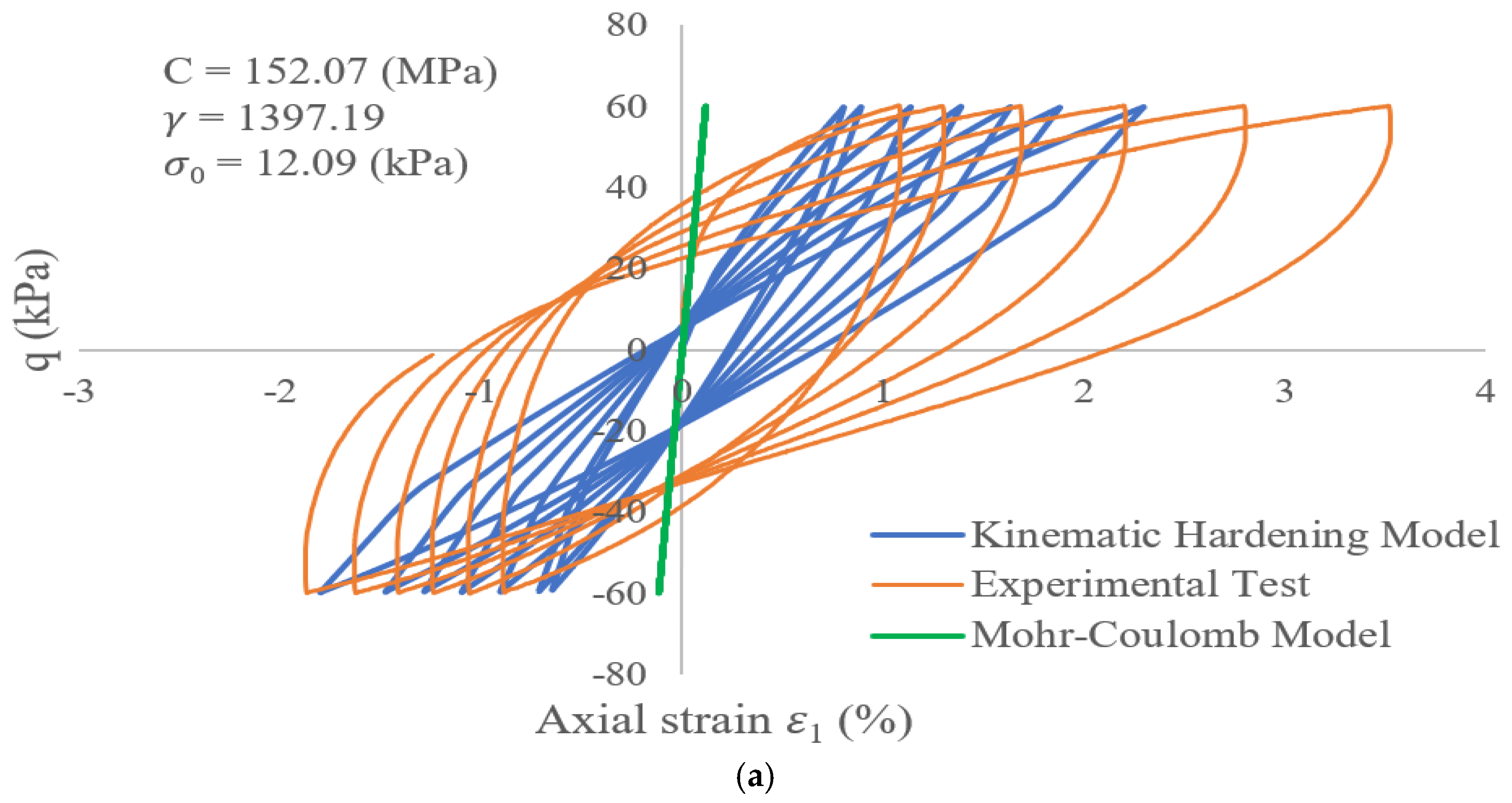
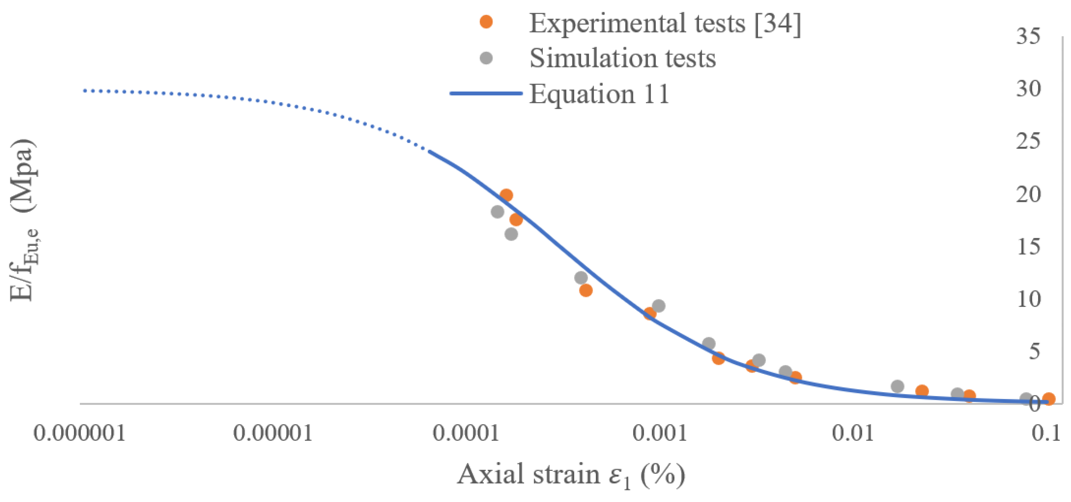
2.2.1. Determination of $C$

We use the results of the undrained cyclic triaxial tests at different stress amplitudes (C1–C8 and C32–C36) [33] to determine the nonlinear undrained Young’s modulus. For instance, Figure 2 shows the deviatoric stress ($q$) and undrained Young’s modulus ($E_u$) versus the axial strain (${\epsilon }_1$) curve with stress amplitudes of 60 kPa and 70 kPa for undrained cyclic triaxial tests of C7 and C8, respectively. Each loading and unloading loop (Figure 2a,c) is used to calculate the undrained Young’s modulus value at the desired strain amplitude, using the equation $E_u=\frac{q^{ampl}}{{\epsilon }_1^{ampl}}$ (Figure 2b,d). Therefore, each point in Figure 2b,d is the value of the undrained Young’s modulus of the corresponding cycle in Figure 2a,c. Thus, Figure 2 depicts the stiffness degradation of soil under cyclic loading and unloading. As shown in the diagrams, by increasing the number of cycles and axial strain amplitudes, the undrained Young modulus or the shear modulus decrease, and the amount of damping caused by the soil plasticity increases. Although by increasing number of cycles the amount of axial strain is also increased, the increase in axial strain on both sides of the horizontal coordinate axis is unequal, such that there is more on the positive side (compression).

Figure 3 shows the normalized undrained Young’s modulus ($\raisebox{1ex}{$E_u$}\!\left/ \!\raisebox{-1ex}{$f_{E,e}$}\right.$) versus strain amplitude (${\epsilon }_1^{ampl}$) based on the results of numerical analysis, Equation (11), and the experimental results of the several undrained cyclic triaxial tests, where these are performed under different stress amplitudes (C1–C8 and C32–C36) [33] to calibrate the parameters $C$ and $\lambda$ of the constitutive model. The calibration of parameter $\lambda$ using the data in Figure 3 is described in Section 2.2.2. Each experiment test [33] is based on a number of specified cycles, and numerical simulations were performed based on the same number of cycles. The parameters of the model have been calibrated in order to best fit the numerical model points with the experimental results. In this figure, the second and fifth cycles of curves of deviatoric stress ($q$) versus axial strain (${\epsilon }_1$) of the undrained cyclic triaxial tests are used to obtain the undrained Young’s modulus values ($E_u$); then, these values are divided by the function of the void ratio (Equation (10)) and plotted versus the corresponding strain amplitude ${\epsilon }_1^{ampl}$.

The equation of the void ratio (used in Figure 3) obtained on the basis of experimental data is presented as follows [33] (Equation (10)):

$$f_{E_u,e}=\frac{{\left(4.4-e\right)}^2}{\left(1+e\right)}$$

(10)

where $e$ is the void ratio of soil.

As shown in Figure 3, by increasing the strain amplitude, the values of the undrained Young’s modulus decrease, and this decreasing trend is proportional to Equation (11) [34]:

$$\frac{E_u}{E_{u_{max}}}=f_{E_u,ampl}=\frac{1}{1+{\left(\raisebox{1ex}{${\epsilon }_1^{ampl}$}\!\left/ \!\raisebox{-1ex}{${\epsilon }_{1,r}^{ampl}$}\right.\right)}^{\alpha }}$$

(11)

where ${\epsilon }_{1,r}^{ampl}=3\ast {10}^{-4}$, corresponding to $\frac{E_u}{E_{u_{max}}}=f_{E_u,ampl}=0.5$ and $\alpha =0.9$ (for kaolin clay) [33]. In addition, by subjecting the experimental data to extrapolation operations, e.g., $E_{u_{max}}\approx 30\ast f_{E_u,e}$, Equations (9)–(11) can be used to express parameter $C$ as follows (Equation (12)):

$$C=E_{u_{max}}=30\ast f_{E_u,ampl}\ast f_{E_u,e}.$$

(12)

Using the results obtained from the undrained cyclic triaxial test at very small strains (${\epsilon }_1^{ampl}<{10}^{-6}$), the value of the maximum undrained Young’s modulus can be calculated.

Then, according to the equation $G_{max}=\frac{E_{u_{max}}}{2\left(1+{\upsilon }_{max}\right)}$, the value of the maximum shear modulus can be obtained, where $E_{u_{max}}$ and ${\upsilon }_{max}$ are the maximum undrained Young’s modulus and Poisson ratio, respectively, and ${\upsilon }_{max}=0.49$ in the undrained case.

2.2.2. Determination of $\lambda$, ${\sigma }_0$, and ${\gamma }_o$

The undrained shear strength ($S_u$) is obtained from the results of a monotonic consolidated undrained triaxial test. Figure 4 shows the stress–strain relationship in the monotonic undrained triaxial test [33]. According to this figure and using the following equation, the maximum value of deviatoric stress and undrained shear strength can be calculated as follows (Equation (13)).

$$S_u=\frac{{\left({\sigma }_1-{\sigma }_3\right)}_{max}}{2}=\raisebox{1ex}{$q_{max}$}\!\left/ \!\raisebox{-1ex}{$2$}\right.$$

(13)

where $S_u$ is the undrained shear strength, ${\sigma }_1$ and ${\sigma }_3$ are the maximum and minimum mean stress, respectively, and the deviatoric stress is $q={\sigma }_1-{\sigma }_3$.

The effective maximum yield stress considering the triaxial test condition is calculated as follows (the detailed expression can be found in Appendix B):

$${\sigma }_y=\frac{2 \sqrt{3}}{3} S_u.$$

(14)

The effective maximum yield stress considering the pure shear test is calculated as follows:

$${\sigma }_y=\sqrt{3} S_u.$$

(15)

The next parameter for calibration is $\lambda$. The first method of calibrating $\lambda$ in the kinematic hardening model is based on the undrained cyclic triaxial test data. The deviatoric stress ($q$) versus axial strain (${\epsilon }_1$) under the stress control condition at different stress amplitudes are plotted based on the simulation results of the undrained cyclic triaxial test, and similar to the experimental method, the undrained elastic modulus ($E_u$) of the second and fifth cycles of each test is obtained. Then, the curve of the undrained Young’s modulus versus axial strain is plotted for both the experimental data and simulation results to calibrate $\lambda$. The simulation results of the undrained cyclic triaxial test and their comparison with the experimental results are presented in Figure 3. Here, $\lambda$ = 0.14 is found to provide a reasonable fit to the experimental results, where the simulation is performed using Abaqus software under the stress control condition.

If undrained cyclic triaxial test data are not available, the results of the cyclic shear test under the strain control condition and the Ishibashi and Zhang experimental equations using the plasticity index of soil are used to calibrate the parameter λ (second method). In this method, the curve data of shear modulus versus shear strain ($G-\gamma$ curve) is required to calibrate this parameter. Thus, the hysteresis loops of the cyclic shear test simulation in different strain amplitudes should first be plotted. For instance, the hysteresis loops of three different strain levels are shown in Figure 5. As can be seen, the value of the damping caused by the soil plasticity increases, and the shear modulus decreases if the strain levels are increased. Then, the shear modulus corresponding to the stabilized cycle is obtained for each strain amplitude to enable the plotting of the $G-\gamma$ points to calibrate $\lambda$ (see Figure 6). For example, the shear stress–strain loops of three strain amplitudes in Figure 5 correspond to the designated points in Figure 6. These two figures illustrate the validation of the kinematic hardening model against the published $G-\gamma$ curve of Ishibashi and Zhang [32]. After calibration using this method, $\lambda$ = 0.12 is obtained.

After determining the parameters $S_u$, ${\sigma }_y$, and $\lambda$, the initial size of yield surface (${\sigma }_0$) is obtained from Equation (7) (${\sigma }_0=\lambda {\sigma }_y$).

The last parameter to be determined is the rate decrease of the kinematic hardening modulus (${\gamma }_o$). According to Figure 1, the amount of effective maximum yield stress is determined by Equation (16):

$${\sigma }_y=\raisebox{1ex}{$C$}\!\left/ \!\raisebox{-1ex}{${\gamma }_o$}\right.+{\sigma }_0.$$

(16)

Finally, from Equations (14)–(16), parameter ${\gamma }_o$ is calculated according to Equations (17) and (18):

$${\gamma }_o=\frac{C}{{\sigma }_y-{\sigma }_0}=\frac{C}{\frac{2 \sqrt{3}}{3} S_u-{\sigma }_0}$$

(17)

(Triaxial test condition)

$${\gamma }_o=\frac{C}{{\sigma }_y-{\sigma }_0}=\frac{C}{\sqrt{3} S_u-{\sigma }_0}$$

(18)

(Simple pure shear test condition).

Generally, the triaxial test is an acceptable method for assessing the cyclic behavior of soils, and usually this test is used to calibrate the parameters of different constitutive models. Applying relatively simple boundary conditions and creating proper meshes in simulations of this test afford logical and reliable results. Thus, the results of the cyclic triaxial test using nonlinear kinematic hardening and Mohr–Coulomb models on a clay sample are compared with the experimental model results to validate and investigate the kinematic hardening constitutive model. This test is modeled in the 2D axisymmetric case to achieve acceptable results. Application of a 200 kPa confining pressure is simulated as a uniformly distributed load applied normally inward to all external elements around the specimen; then, the cyclic load ($q=60\mathrm{kPa}\&70\mathrm{kPa}$) is applied to the top of the sample.

In the Mohr–Coulomb model, since the test is carried out in an undrained condition (i.e., an undrained cyclic triaxial test), the internal friction angle of soil ($\phi$) is zero and the cohesion value ($C$) equals the undrained shear strength of soil ($S_u$). Figure 7 shows the comparison of deviatoric stress versus axial strain in numerical simulations (kinematic hardening model and Mohr–Coulomb) with the experimental results in stress control mode. As shown in the diagrams, the behavior of undrained soils using the kinematic hardening model is in relatively good agreement with the results obtained from the experimental test, while the Mohr–Coulomb model fails to create the hysteresis loops, and the results thus differ from the experimental results. In addition, the material behavior in the Mohr–Coulomb model is in the elastic range.

It is worth noting that this numerical simulation for the Mohr–Coulomb model is performed in two modes without considering and taking into account the damping ratios, and the results of the two cases are similar, which indicates that the linear elastic–perfectly plastic Mohr–Coulomb model cannot accurately predict the soil behavior under cyclic loading. In contrast, the kinematic model is capable of creating hysteresis loops and considers the soil stiffness degradation as the number of loading cycles increases. As shown in Figure 7, the undrained Young’s modulus ratio of the numerical model to the experimental model ($\frac{E_{u\left(\mathrm{NemericalModel}\right)}}{E_{u\left(\mathrm{ExperomentalModel}\right)}}$) increases with an increasing number of loading cycles, so that in the last cycle, it reaches its maximum value of approximately 1.4. Thus, a numerical model generally overestimates the soil stiffness degradation. The experimental curves in Figure 7 are related to tests C7 and C8.

Finally, after calibrating and using the corresponding equations, the values of the different hardening parameters are calculated for all five soil layers (see Figure 8). Thus, the values of the constitutive model parameters used in all of the analyses can be calibrated according to the second method (

Table 1. Parameters of the constitutive model.

Layer No.	Soil Type	${\mathit{G}}_0$ (MPa)	$\mathit{E}$ (MPa)	${\mathit{\sigma }}_{\mathit{y}}$ (kPa)	${\mathit{\sigma }}_0$ (kPa)	$\mathit{C}$ (MPa)	$\mathit{\lambda }$	$\mathit{\gamma }$
1 (top)	Silty clay	28.38	84.58	51.79	5.18	84.58	0.1	1814.63
2	Very soft silty clay	24.73	73.7	47.46	5.7	73.7	0.12	1764.85
3	Very soft clay	24.28	72.35	34.29	4.46	72.35	0.13	2425.41
4	Clay	37.76	112.52	45.55	5.47	112.52	0.12	2807.38
5	Silty clay	71.52	211.7	51.96	5.72	211.7	0.11	4578.29

).

3. Finite Element Models

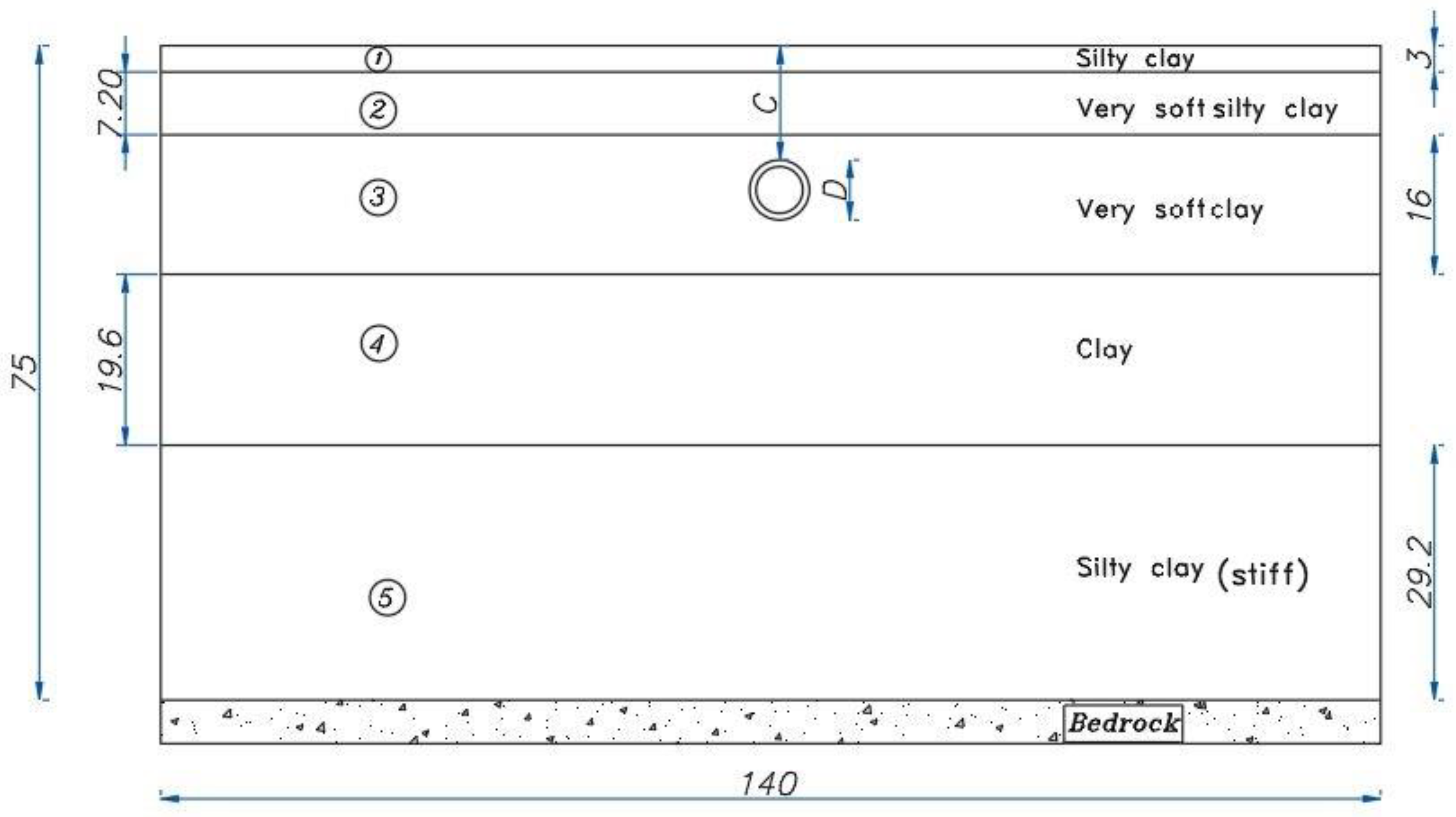
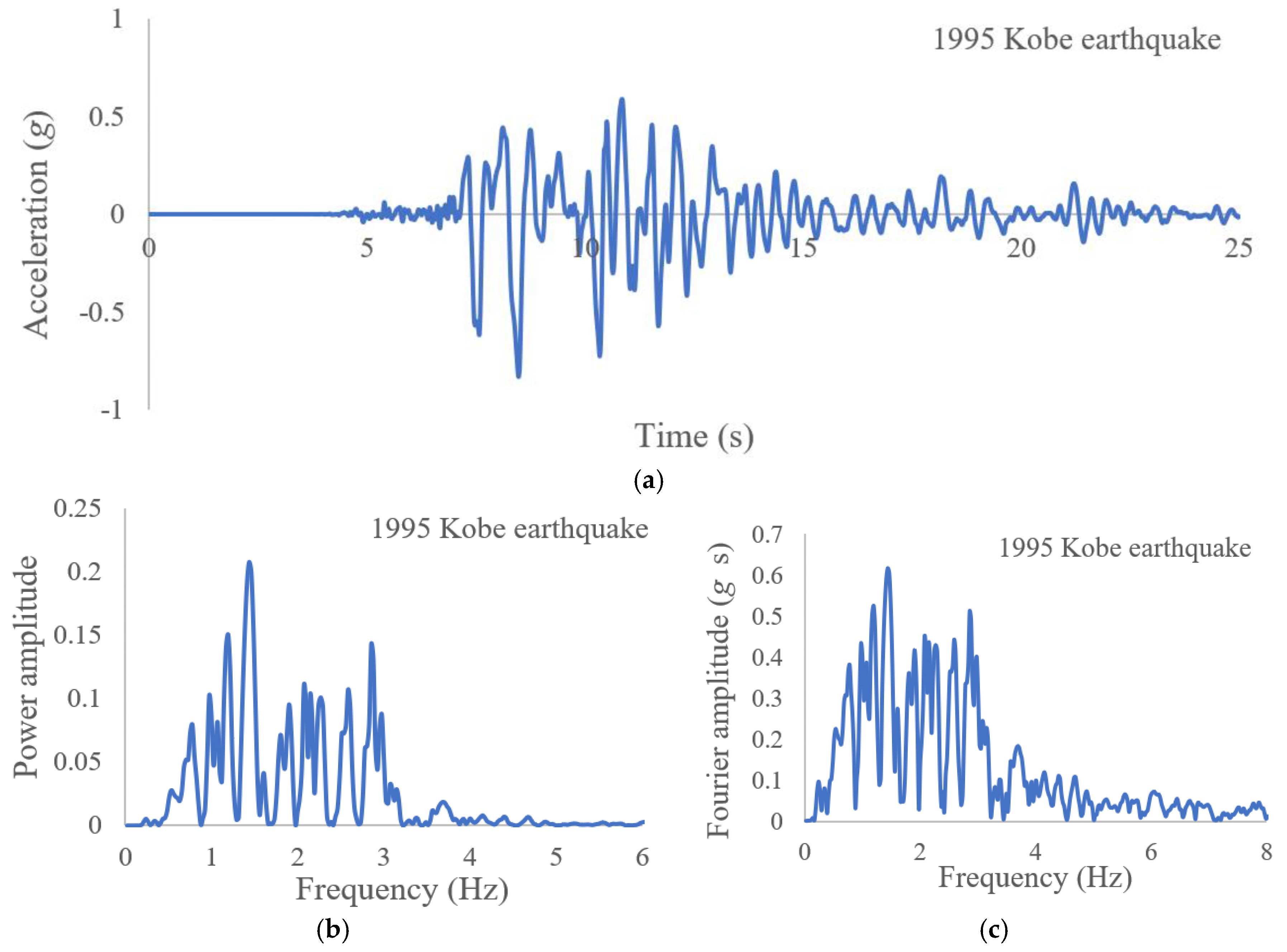
3.1. Model Descriptions

As previously mentioned, many factors—such as the type and thickness of soil, shape, dimensions, and depth of a tunnel, as well as earthquake intensity—affect the seismic response of a tunnel to an earthquake. In this study, we aim to examine the effect of these factors on the seismic behavior of a tunnel and compare the results with those from previous studies performed using a linear elastic–perfectly plastic Mohr–Coulomb model [29]. In all of the studied models, five layers of soft soil are used with different characteristics and various thicknesses of 29.2 m, 19.6 m, 16 m, 7.2 m, and 3 m, corresponding to structural layers from bedrock to the soil surface, respectively. The schematic configuration of the models, including the soil layers and tunnel used in all of the analyses, is given in Figure 8, and the properties of the clay soils used in this study are summarized in

Table 2. Properties of the clay soils.

Layer No.	Layer Thickness (m)	Unit Weight γ (kN/m3)	Undrained Shear Strength Su (kPa)	Poisson’s Ratio ν	Damping Ratio α	Damping Ratio β
1 (top)	3.00	18.40	29.90	0.49	9.6600	0.7764 × 10−3
2	7.20	17.50	27.40	0.49	3.8930	1.9260 × 10−3
3	16.00	16.90	19.80	0.49	1.7710	4.2380 × 10−3
4	19.60	18.00	26.30	0.49	1.7440	4.3010 × 10−3
5	29.20	18.10	30.00	0.48	1.7060	4.3970 × 10−3

.

A circular tunnel with a diameter of 6 m and a square tunnel with a length of 5.3 m are used to investigate the effect of the shape of the tunnel on the dynamic response. Different tunnel-lining thicknesses of the circular tunnel are also considered to study the effect of lining thickness on the seismic response. The properties of the concrete used in the tunnel lining are given in

Table 3. Properties of the concrete used in the tunnel lining.

Material	Density (kN/m3)	Elastic Modulus (GPa)	Poisson’s Ratio ν	Damping Ratio α	Damping Ratio β
Concrete	25	30	0.20	2.2544	0.000908

.

One of the factors affecting the seismic behavior of a tunnel is the intensity of the earthquake force imposed on the soil–tunnel model. The earthquake load applied to the base of models is that of the 1995 Kobe earthquake, i.e., 0.83 g PGA (peak ground acceleration) (as recorded at KJMA station); then, this is scaled down to 0.4 g to investigate the effect of this parameter on the dynamic soil–tunnel behavior. There are various methods [35,36,37,38,39] used for the boundary conditions of models to ensure that these conditions prevent the return of earthquake waves, and we use the viscous spring boundary method to surround our soil models. The acceleration time history of the Kobe earthquake, and the power amplitude and Fourier amplitude spectra used in this study, are presented in Figure 9.

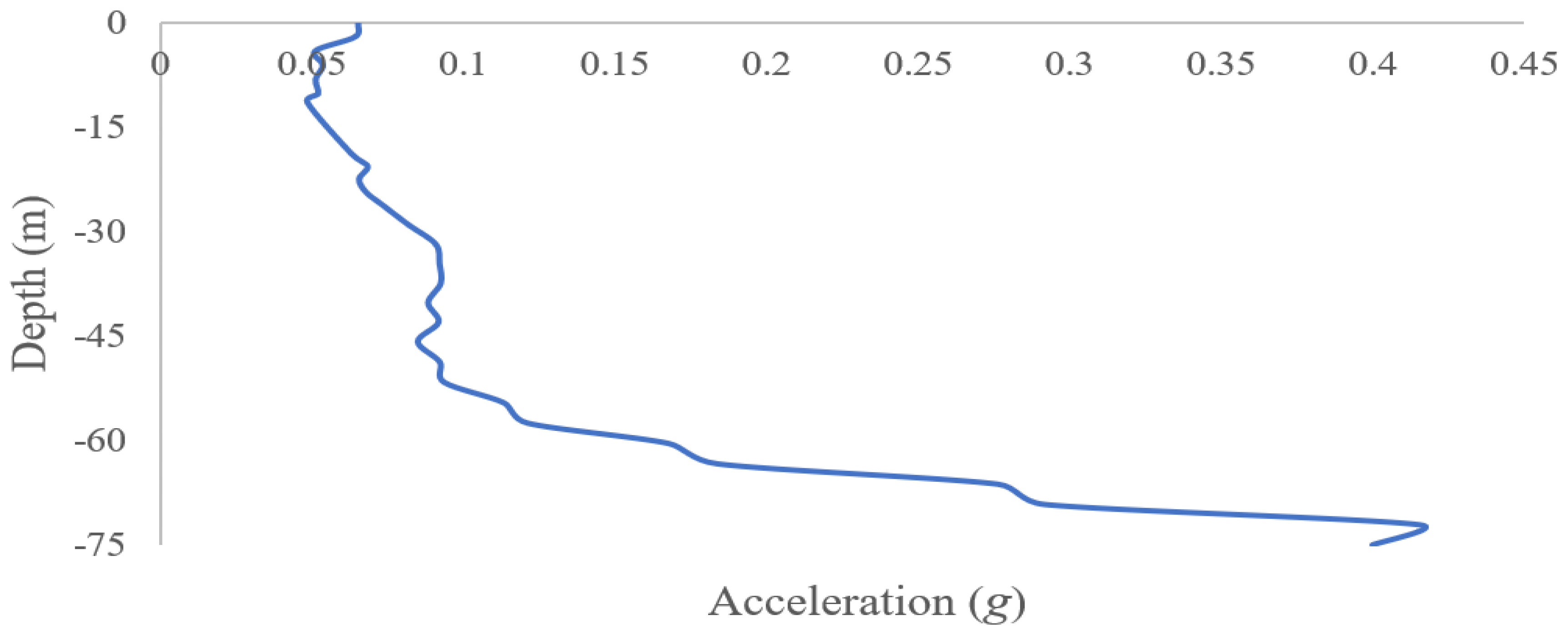
3.2. Results and Discussions

In this study, the linearly elastic–perfectly plastic model and the kinematic hardening constitutive model are used to model soil behavior under earthquake load and some of the parameters that affect the seismic behavior of tunnels are investigated. The results that we obtain from a nonlinear kinematic hardening model are compared with those of a previous study (performed using a Mohr–Coulomb model) [29]. It is noteworthy that in this research, all the soil–tunnel models were simulated in addition to the kinematic hardening constitutive model using the Mohr–Coulomb model, and the results were in good agreement with the results of a previous study that considered the Mohr–Coulomb model using PLAXIS software. The results we obtain are discussed below.

To investigate the effect of tunnel embedment depth on the seismic response of a soil–tunnel system, a circular tunnel with a diameter of 6 m (D = 6 m) at depths of 6, 12, and 18 m (C1 = 6 m, C2 = 12 m, and C3 = 18 m) is subject to Kobe earthquake force with a maximum acceleration of 0.4 g to examine the effect of the interaction between soil and tunnel. Figure 10 shows the maximum acceleration response of the earthquake to the soil depth; as can be seen, the earthquake acceleration response decreases from the bedrock to the soil surface. Therefore, the forces that are exerted on deeper tunnels are larger.

The bending moment created in the tunnel lining is also investigated to determine the effect of tunnel depth on the seismic response. Figure 11 shows the bending moment created in a node on the lining at three different depths (6 m, 12 m, and 18 m) by considering the kinematic hardening model. The bending moment increases with increasing tunnel depth, which indicates an increase in the forces applied to the tunnel lining, i.e., the earthquake force increases with depth (see Figure 10). Figure 12 shows the comparison of tunnel displacement (considering the top node of the tunnel lining) at three different depths during the earthquake loading. As the tunnel depth increases, its displacement decreases, which means that the shallow tunnel experiences the largest displacement.

The acceleration response curve on the soil surface (at the center line of the model) for a tunnel at different depths (C1 = 6 m, C2 = 12 m, and C3 = 18 m) is shown in Figure 13, illustrating the effect of tunnel depth on the acceleration response of the soil surface. This graph results from a model in which the thickness of the tunnel lining is 0.3 m and the input motion of earthquake is 0.4 g. According to Figure 13, the maximum acceleration response on the soil surface does not change with increasing depth, and the value of maximum acceleration for all depths is approximately 0.06 g.

Three lining thicknesses (t1 = 0.15 m, t2 = 0.30 m, and t3 = 0.45 m) are considered for a circular tunnel of diameter 6 m to study the effect of the tunnel-lining thickness on its seismic behavior under the Kobe earthquake load. Figure 14 is based on the bending moment (normalized to the radius of the tunnel and the free-field shear stress ($\frac{M}{\tau R^2}$), ($\tau =G{\gamma }_{max}$)) in terms of the lining thickness ratio ($\raisebox{1ex}{$t$}\!\left/ \!\raisebox{-1ex}{$D$}\right.$), and it shows a comparison of the results of this study using the nonlinear kinematic hardening and Mohr–Coulomb models with those of a previous study [29]. Based on these results, it can be seen that the tunnel-lining thickness affects the bending moment that occurs in the lining because the relative stiffness (i.e., the lining stiffness relative to the surrounding soil stiffness) varies with changes in the lining thickness. This means that the bending moment increases with the increasing lining thickness, indicating that the lining is able to withstand greater forces when it has a greater thickness. For instance, in the kinematic hardening model, with a tunnel depth of 12 m ($D=12$ m) and an earthquake acceleration of 0.4 g, the maximum bending moment created on the lining thicknesses of 0.15 m, 0.30 m and 0.45 m are 22,990 N.m, 53,180 N.m, and 68,240 N.m, respectively.

The earthquake forces of 0.4 g and 0.83 g are applied to the soil–tunnel system with a tunnel depth and thickness of 12 m and 0.3 m, respectively, to investigate the effect of the earthquake intensity on soil behavior. The distribution of equivalent plastic strain created near the tunnel for both the Mohr–Coulomb and kinematic hardening models is shown in Figure 15. Under the same conditions, the maximum equivalent plastic strain created in the soil elements in contact with the lining in the Mohr–Coulomb model is more than the kinematic hardening model, because the Mohr–Coulomb model cannot incorporate the damping caused by the soil plasticity. This means that the maximum value in the kinematic hardening model under 0.83 g (${\epsilon }_p=$ 0.0143) is approximately equal to the Mohr–Coulomb model under 0.4 g (${\epsilon }_p=$ 0.0126), but in the Mohr–Coulomb model, the equivalent plastic strain is zero in the soil elements away from the tunnel lining. Therefore, the Mohr–Coulomb model is not suitable for modeling soil under seismic loading, as it fails to generate loading and unloading loops, and it is unable to show the actual behavior of the soil. For instance, the equivalent plastic strain created during the earthquake loading (0.4 g and 0.83 g) for a node on the soil (above the tunnel crown) for both the Mohr–Coulomb and kinematic models is shown in Figure 16.

The choice of the shape and dimensions of a tunnel depends on its intended purpose. For example, circular, quadrilateral and horseshoe cross-section shapes are used for railways tunnels, and each of these tunnels exhibits different behavior under seismic loads. Here, we study two circular and square tunnels with the same embedment depth (D = 12 m) and lining thickness (t = 0.30 m), which are subject to the same earthquake intensity (0.4 g), to investigate the effect of tunnel shape on the seismic behavior. The difference between the results we obtain and those from the previous study [29] (Figure 17) are due to the different constitutive model used.

The maximum bending moment generated at all nodes on the tunnel lining for both Mohr–Coulomb and kinematic hardening models are shown in Figure 17a,b, which are for the circular tunnel and square tunnel, respectively. The horizontal axis of these graphs indicates the perimeter of the tunnel (zero corresponds to the top point of the tunnel, and other points are selected based on their clockwise-perimeter distance from the top point). Figure 18 shows the comparison of the bending moment created for one node on the top of the circular tunnel (tunnel crown) during the earthquake loading for both constitutive models. According to Figure 17a,b and Figure 18, there is a relatively large difference between the results of the two models, so that in the Mohr–Coulomb model, the absolute of the bending moment values at all nodes is more than that of the nonlinear kinematic hardening model. The results obtained from this study of the effect of the tunnel shape on the seismic behavior show that the maximum bending moment generated on the perimeter of the square tunnels is more than that generated on the perimeter of circular tunnel. It also shows that the corners of the square tunnel have maximum values, proving that the circular tunnel performs better than the square tunnel under the applied seismic loads.

4. Conclusions

The use of advanced constitutive models is limited in practice due to the difficulty in calibrating several constitutive parameters. Here, a linear elastic model is used for tunnels, and a linear elastic–perfectly plastic Mohr–Coulomb model and a nonlinear kinematic hardening model are used as advanced constitutive models for clay soil. Two different methods—one using data from a cyclic shear test simulation and the experimental curve of Ishibashi and Zhang [32] and the other using experimental data and some data from a simulation of an undrained cyclic triaxial test (which is a new method)—are used to calibrate the parameters of a kinematic hardening constitutive model. The results of this research can be summarized as follows.

• Choosing the appropriate constitutive model to achieve logical results is key to evaluating the seismic behavior of the tunnel in numerical methods. The use of a nonlinear kinematic hardening model that considers the effect of soil stiffness degradation is appropriate for structures under cyclic loads.
• Calibrating the parameters of the kinematic hardening constitutive model using the data from undrained cyclic triaxial tests afford results that are almost identical to those from using the Ishibashi and Zhang equations and data from simulation of the cyclic shear tests.
• The nonlinear kinematic hardening constitutive model can better demonstrate the cyclic deformation behavior of soils under cyclic loading than conventional and simple models such as the linear elastic–perfectly plastic Mohr–Coulomb model.
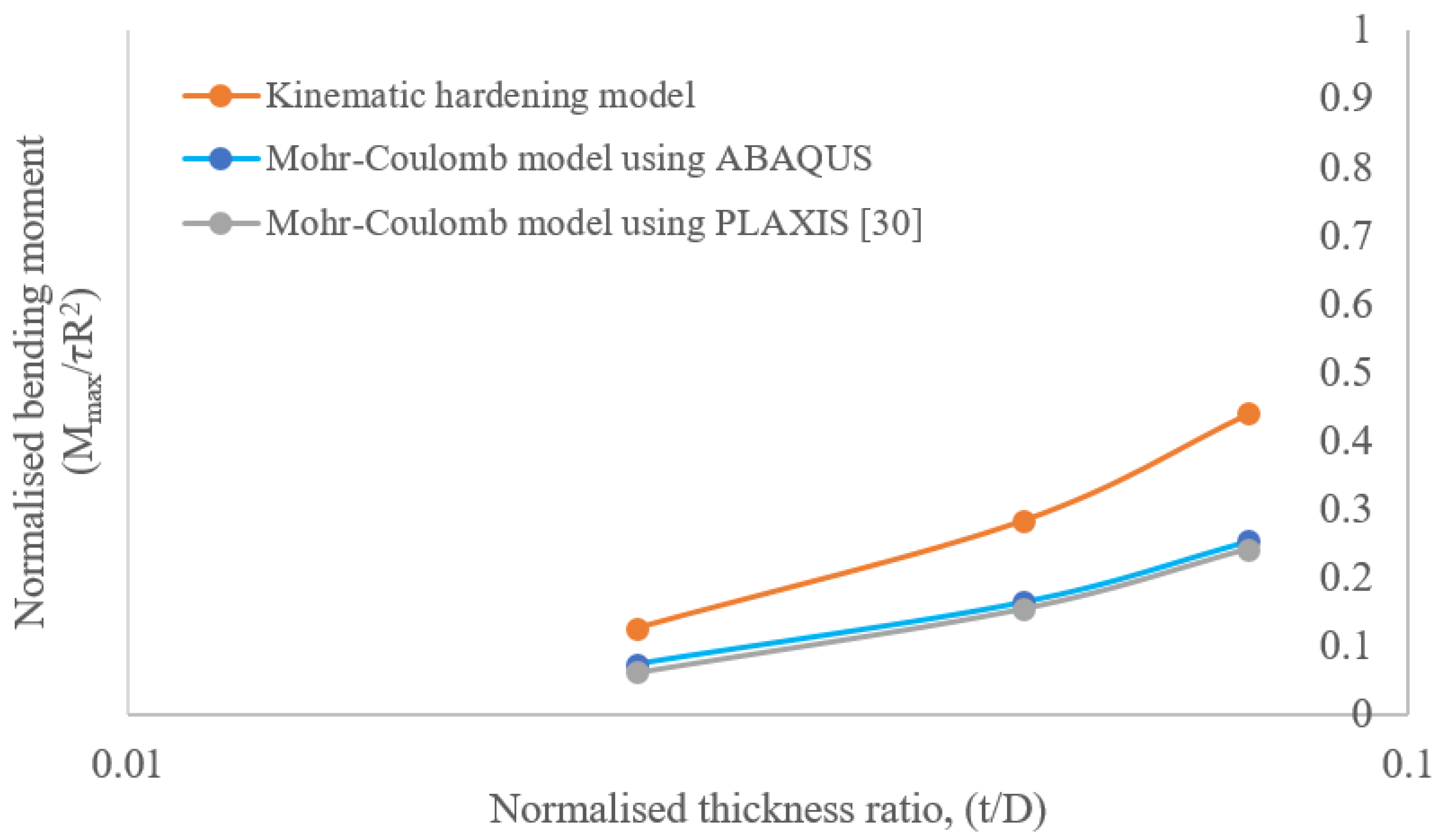
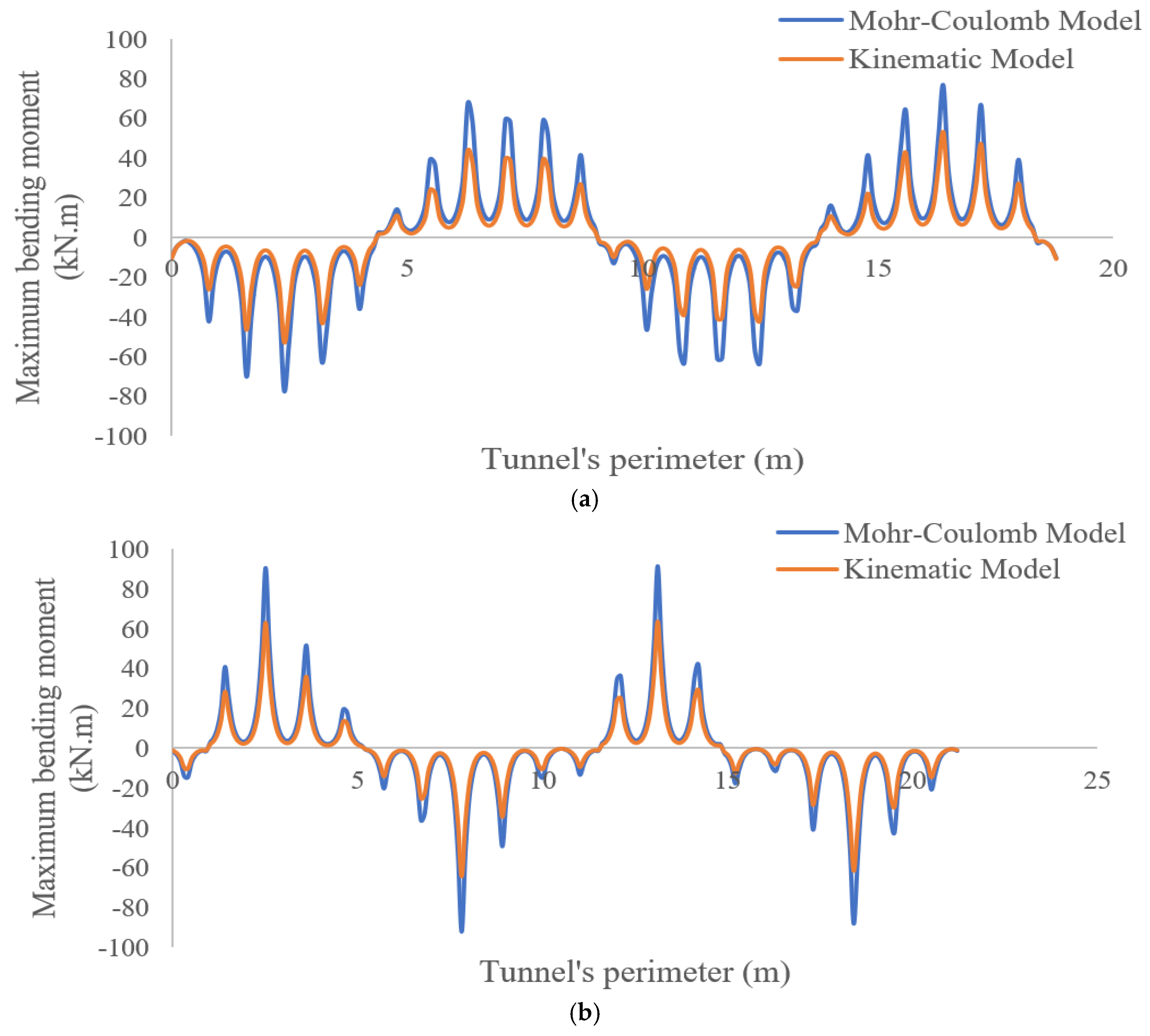
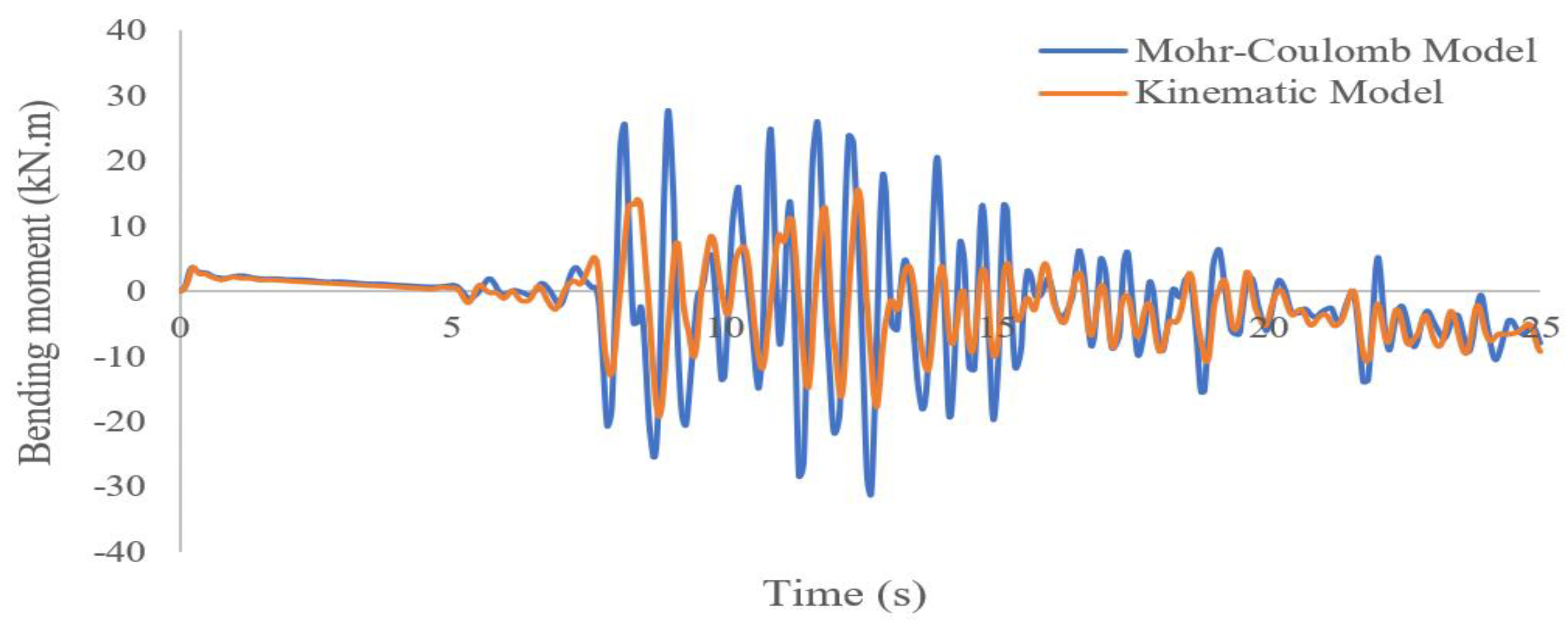
• The Mohr–Coulomb model overestimates the design and it is not economically acceptable. For example, the bending moments created in the tunnel lining are much larger in the Mohr–Coulomb model than in the kinematic model.
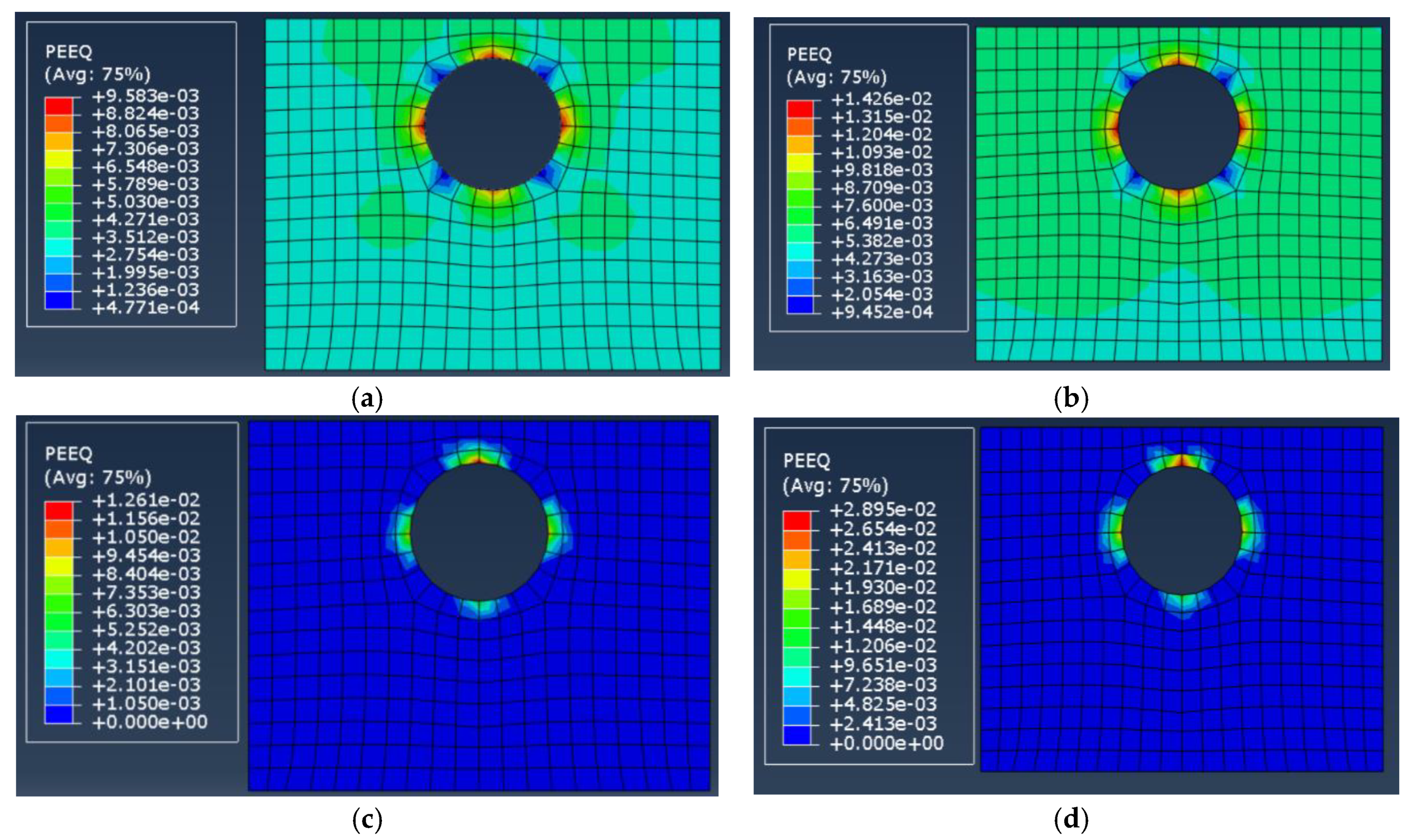
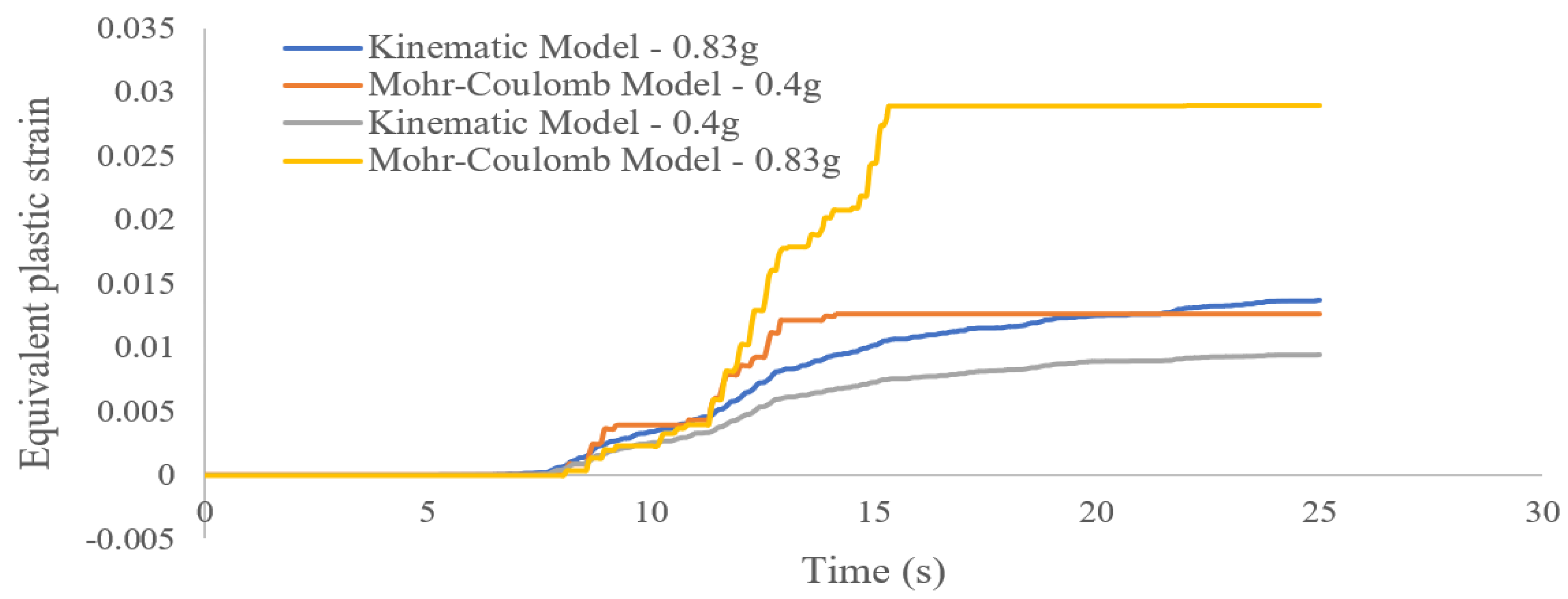
• The plastic strain of soil increases in both the kinematic hardening and Mohr–Coulomb models as the intensity of the earthquake increases from 0.4 to 0.83 g, but this increase is greater in the Mohr–Coulomb model due to its inability to create of hysteresis loops. Therefore, the Mohr–Coulomb model can’t be used to accurately predict the behavior of soil under earthquake loading.
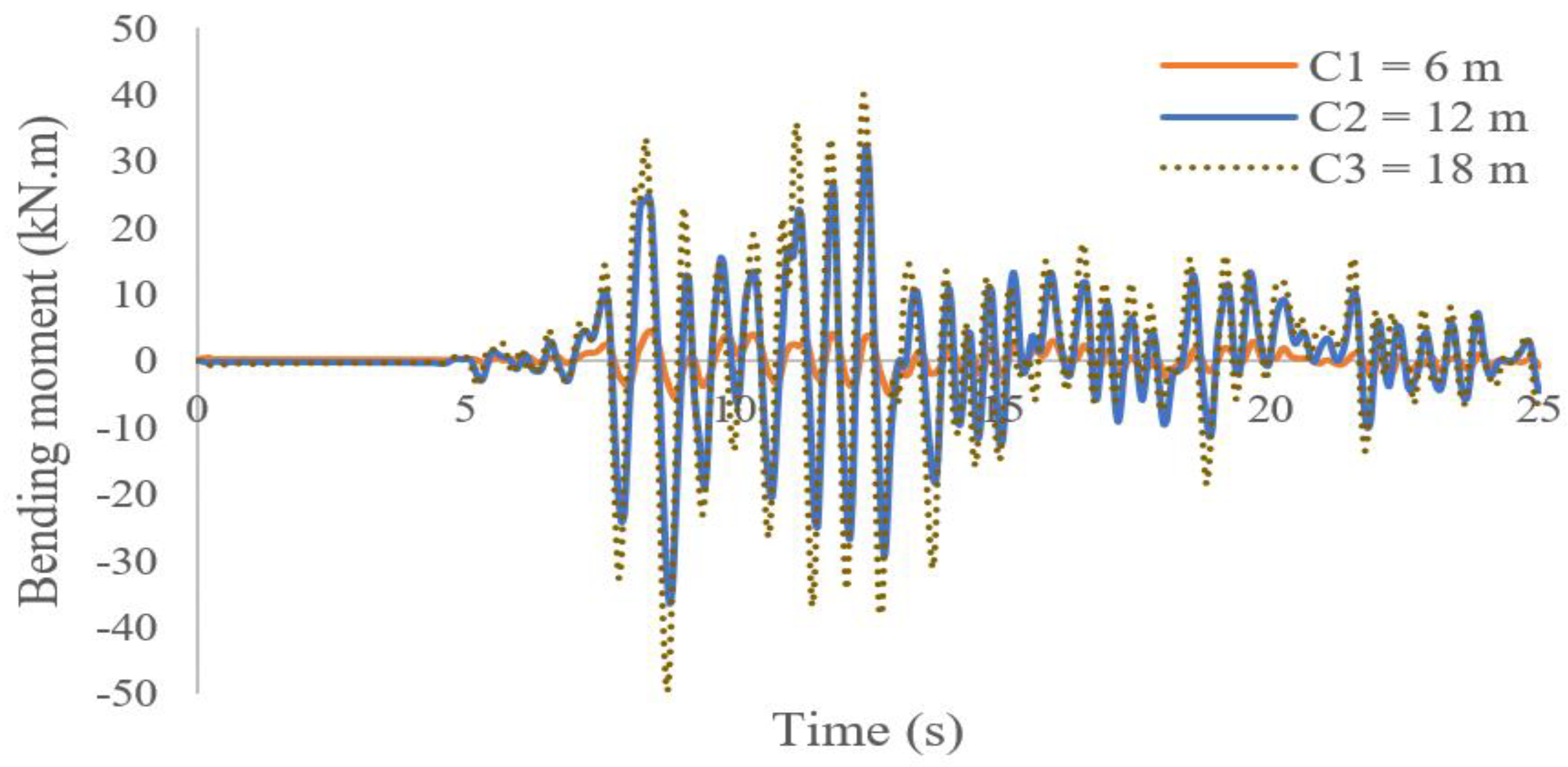
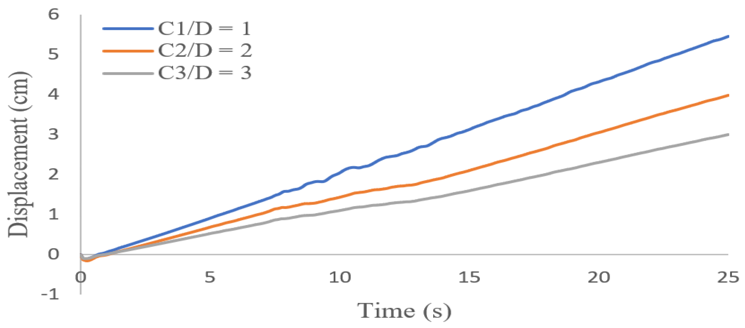
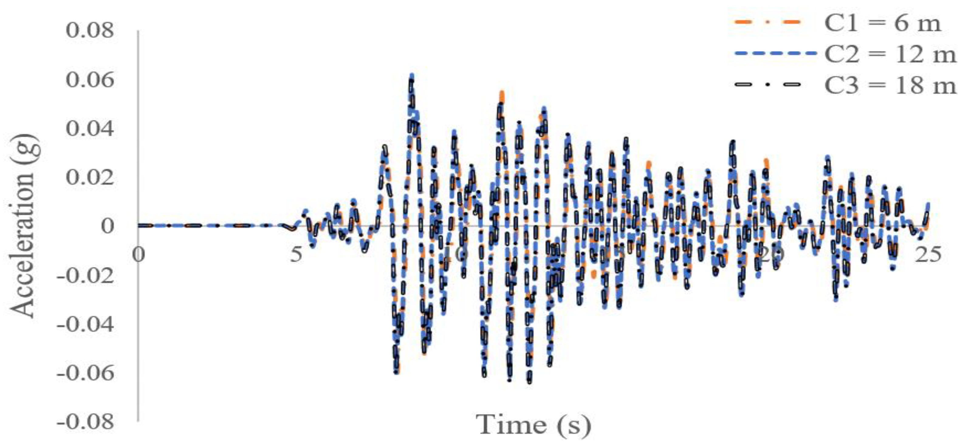
• Changing the depth of a tunnel has no effect on the maximum acceleration response on the soil surface, but as the depth increases, greater forces are applied to the lining, and the bending moment created on the tunnel lining also increases. The lining displacement also decreases with the increasing tunnel depth.
• Another parameter that affects the dynamic behavior of tunnels is the tunnel-lining thickness. The bending moment in the tunnel lining increases with its thickness so that as the dimensions of the tunnel increase, the EI increases and the structure becomes more stiff and able to withstand more forces. The resistance to deformation and the flexibility also increase under dynamic loads.
• The shape of the tunnel dictates the overall response of the soil–tunnel system under dynamic loads. Circular tunnels show better performance than square tunnels against seismic loads. Generally, rounding the corners in square tunnels causes the tunnels to perform better under the imposed loads.

References

1. Asheghabadi, M.S.; Ali, Z. Infinite element 1 boundary conditions for dynamic models under. Indian J. Phys. 2019. [Google Scholar]
2. Castellanos, A.; Romero, M.; Guzman, N. Near shore seismic movements induced by seaquakes using the boundary element method. Earthq. Eng. Eng. Vib. 2017, 16, 571–585. [Google Scholar] [CrossRef]
3. Xu, Q.; Chen, J.; Li, J.; Fan, S. New artificial boundary condition for saturated soil foundations. Earthq. Eng. Eng. Vib. 2012, 11, 139–147. [Google Scholar] [CrossRef]
4. Asheghabadi, M.S.; Sahafnia, M.; Bahadori, A.; Bakhshayeshi, N. Seismic behavior of suction caisson for the offshore wind turbine to generate more renewable energy. Int. J. Environ. Sci. Technol. 2019, 16, 2961–2972. [Google Scholar] [CrossRef]
5. Dawen, G.; Baipo, Y. A two-step explicit finite element method in time domain for 3D dynamic SSI analysis. Earthq. Eng. Eng. Vib. 2011, 31, 9–17. [Google Scholar]
6. Nakamura, S.; Yoshida, N.; Iwatate, T. Damage to Daikai subway station during the 1995 Hyogoken–Nambu earthquake and its investigation. Doboku Gakkai Ronbunshu J-Stage 1996, 537, 287–295. [Google Scholar]
7. Yoshida, N. Damage to subway station during the 1995 Hyogoken-Nambu (Kobe) earthquake. In Earthquake Geotechnical Case Histories for Performance-Based Design; Kokusho, T., Ed.; CRC Press: Tokyo, Japan, 2009; pp. 373–389. [Google Scholar]
8. Ueng, T.S.; Lin, M.L.; Chen, M.H. Some geotechnical aspects of 1999 Chi-Chi, Taiwan earthquake. In Proceedings of the Fourth International Conference on Recent Advances in Geotechnical Earthquake Engineering and Soil Dynamics SPL-10. 1, San Diego, CA, USA, 26–31 March 2001; pp. 1–5. [Google Scholar]
9. Wang, W.; Ren, Q. General introduction to the effect of active fault on deeply buried tunnel. Earthq. Eng. Eng. Vib. 2006, 26, 175–180. [Google Scholar]
10. Kontoe, S.; Zdravkovic, L.; Potts, D.M.; Menkiti, C.O. On the relative merits of simple and advanced constitutive models in dynamic analysis of tunnels. Geotechnique 2011, 61, 815–829. [Google Scholar] [CrossRef] [Green Version]
11. O’Rourke, T.D.; Goh, S.H.; Menkiti, C.O.; Mair, R.J. Highway tunnel performance during the 1999 Düzce earthquake. In Proceedings of the 15th International Conference on Soil Mechanics and Geotechnical Engineering, Istanbul, Turkey, 27–31 August 2001. [Google Scholar]
12. Liu, Y.; Quek, E.J.; Lee, F.H. Translation random field with marginal beta distribution in modeling material properties. Struct. Saf. 2016, 61, 57–66. [Google Scholar] [CrossRef]
13. Matinmanesh, H.; Saleh Asheghabadi, M. Seismic analysis on soil-structure interaction of buildings over sandy soil. In Proceedings of the The Twelfth East Asia-Pacific Conference on Structural Engineering and Construction (EASEC-12), Hong Kong, China, 26–28 January 2011; pp. 24–26. [Google Scholar]
14. Banerjee, S.; Goh, S.H.; Lee, F.H. Earthquake-induced bending moment in fixed-head piles in soft clay. Ge´otechnique 2014, 64, 431–446. [Google Scholar] [CrossRef]
15. Mayoral, J.M.; Alberto, Y.; Mendoza, M.J.; Romo, M.P. Seismic response of an urban bridge-support system in soft clay. Soil Dyn. Earthq. Eng. 2009, 29, 925–938. [Google Scholar] [CrossRef]
16. Saleh Asheghabadi, M.; Rahgozar, M.A. Finite element seismic analysis of soil–tunnel interactions in clay soils. Iran J. Sci. Technol. Trans. Civ. Eng. 2019, 43, 835–849. [Google Scholar] [CrossRef]
17. Asheghabadi, M.S.; Matinmanesh, H. Finite Element Seismic Analysis of Cylindrical Tunnel in Sandy Soils with Consideration of Soil-Tunnel Interaction. Procedia Eng. 2011, 14, 3162–3169. [Google Scholar] [CrossRef]
18. Zhang, L.; Liu, Y. Numerical investigations on the seismic response of a subway tunnel embedded in spatially random clays. Undergr. Space 2020, 5, 43–52. [Google Scholar] [CrossRef]
19. Power, M.; Rosidi, D.; Kaneshiro, J.; Gilstrap, S.; Chiou, S.J. Summary and Evaluation of Procedures for the Seismic Design of Tunnels; Final Report for Task 112-d-5. 3(c); National Center for Earthquake Engineering Research: Buffalo, NY, USA, 1998. [Google Scholar]
20. Li, Y.; Zhao, M.; Xu, C.-S.; Du, X.L.; Li, Z. Earthquake input for finite element analysis of soil-structure interaction on rigid bedrock. Tunn. Undergr. Space Technol. 2018, 79, 250–262. [Google Scholar] [CrossRef]
21. Lanzano, G.; Bilotta, E.; Russo, G.; Silvestri, F. Experimental and numerical study on circular tunnels under seismic loading. Eur. J. Environ. Civ. Eng. 2015, 19, 539–563. [Google Scholar] [CrossRef]
22. Tsinidis, G.; Rovithis, E.; Pitilakis, K.; Chazelas, J.L. Seismic response of box-type tunnels in soft soil: Experimental and numerical investigation. Tunn. Undergr. Space Technol. 2016, 59, 199–214. [Google Scholar] [CrossRef]
23. Ulgen, D.; Saglam, S.; Ozkan, M.Y. Dynamic response of a flexible rectangular underground structure in sand: Centrifuge modeling. Bull. Earthq. Eng. 2015, 13, 2547–2566. [Google Scholar] [CrossRef]
24. Chen, G.; Wang, Z.; Zuo, X.; Du, X.; Gao, H. Shaking table test on the seismic failure characteristics of a subway station structure on liquefiable ground. Earthq. Eng. Struct. Dyn. 2013, 42, 1489–1507. [Google Scholar] [CrossRef]
25. Debiasi, E.; Gajo, A.; Zonta, D. On the seismic response of shallow-buried rectangular structures. Tunn. Undergr. Space Technol. 2013, 38, 99–113. [Google Scholar] [CrossRef]
26. Patil, M.; Choudhury, D.; Ranjith, P.G.; Zhao, J. A numerical study on effects of dynamic input motion on response of tunnel-soil system. In Proceedings of the 16th World Conference on Earthquake Engineering (16th WCEE 2017), Santiago, Chile, 9–13 January 2017; p. 3313. [Google Scholar]
27. Bao, X.; Xia, Z.; Ye, G.; Fu, Y.; Su, D. Numerical analysis on the seismic behavior of a large metro subway tunnel in liquefiable ground. Tunn. Undergr. Space Technol. 2017, 66, 91–106. [Google Scholar] [CrossRef]
28. Cremer, C.; Pecker, A.; Davenne, L. Cyclic macro-element for soil-structure interaction: Material and geometrical non-linearities. Int. J. Numer. Anal. Methods Geomech. 2001, 25, 1257–1284. [Google Scholar] [CrossRef]
29. Frederick, C.O.; Armstrong, P.J. A Mathematical Representation of the Multi Axial Bauschinger Effect; CEGB Report RD/B/N 731; Central Electricity Generating Board, Materials at High Temperatures; Elsevier: Amsterdam, The Netherlands, 2007; Volume 24, pp. 1–23. [Google Scholar] [CrossRef] [Green Version]
30. Chaboche, J.L. A review of some plasticity and viscoplasticity constitutive theories. Int. J. Plast. 2008, 24, 1642–1693. [Google Scholar] [CrossRef]
31. Zakavi, S.J.; Zehsaz, M.; Eslami, M.R. The ratchetting behavior of pressurized plain pipework subjected to cyclic bending moment with the combined hardening model. Nucl. Eng. Des. 2010, 240, 726–737. [Google Scholar] [CrossRef]
32. Chaboche, J.L.; Nouailhas, D. Constitutive modeling of ratcheting effects-part I: Experimental facts and properties of the classical models. J. Eng. Mater. Technol. Trans. Asme 1998, 111, 384. [Google Scholar] [CrossRef]
33. Anastasopoulos, I.; Gelagoti, F.; Kourkoulis, R.; Gazetas, G. Simplified constitutive model for simulation of cyclic response of shallow foundations: Validation against laboratory tests. J. Geotech. Geoenviron. Eng. 2011, 137, 1154–1168. [Google Scholar] [CrossRef] [Green Version]
34. Patil, M.; Choudhury, D.; Ranjith, P.G.; Zhao, J. Behavior of shallow tunnel in soft soil under seismic conditions. Tunn. Undergr. Space Technol. 2018, 82, 30–38. [Google Scholar] [CrossRef]
35. Lemaitre, J.; Chaboche, J.L. Mechanics of Solid Materials; Cambridge University Press, 1994; 584p, ISBN 0521477581. [Google Scholar]
36. Smith, C.; Kanvinde, A.; Deierlein, G. Calibration of Continuum Cyclic Constitutive Models for Structural Steel Using Particle Swarm Optimization. J. Eng. Mech. 2017, 143, 04017012. [Google Scholar] [CrossRef]
37. Ishibashi, I.; Zhang, X. Unified dynamic shear moduli and damping ratios of sand and clay. Soils Found. 1993, 33, 182. [Google Scholar] [CrossRef] [Green Version]
38. Wichtmann, T.; Triantafyllidis, T. Monotonic and cyclic tests on kaolin: A database for the development, calibration and verification of constitutive models for cohesive soils with focus to cyclic loading. Acta Geotech. 2018, 13, 1103–1128. [Google Scholar] [CrossRef]
39. Stokoe, K.H.; Darendeli, M.B.; Andrus, R.D.; Brown, L.T. Dynamic soil properties: Laboratory, field and correlation studies. In Proceedings of the 2nd International Conference on Earthquake Geotechnical Engineering, Lisboa, Portugal, 21–25 June 1999; Volume 3, pp. 811–845. [Google Scholar]
Figure 1. Simplified 1D representation of a kinematic hardening process.
Applsci 10 02834 g001
Figure 2. Deviatoric stress and undrained Young’s module vs. axial strain: (a,b) test C7 with p 0 = 200   kPa , q a m p l = 60   kPa , e = 1.202 ; (c,d) test C8 with p 0 = 200   kPa , q a m p l = 70   kPa , e = 1.202 [33].
Applsci 10 02834 g002
Figure 3. Calibration of parameters C and λ .
Applsci 10 02834 g003
Figure 4. Stress–strain relationship in the monotonic triaxial test ( q and S u ) [33].
Applsci 10 02834 g004
Figure 5. Hysteresis loops of a cyclic simple shear test at different strain levels: (a) engineering shear strain vs. time, (b) γ = 0.001 , (c) γ = 0.007 , (d) γ = 0.01 .
Applsci 10 02834 g005
Figure 6. Comparison of an Finite Element-computed G γ curve with the experimental curve of Ishibashi and Zhang (1993).
Applsci 10 02834 g006
Figure 7. Comparison of the kinematic hardening model and Mohr–Coulomb model with experimental test data: (a) q = 60   kPa , (b) q = 70   kPa .
Applsci 10 02834 g007aApplsci 10 02834 g007b
Figure 8. The soil–tunnel system.
Applsci 10 02834 g008
Figure 9. Characteristics of the 1995 Kobe earthquake: (a) the acceleration time history; (b) the power amplitude; (c) the Fourier amplitude spectrum.
Applsci 10 02834 g009
Figure 10. Maximum acceleration response with depth.
Applsci 10 02834 g010
Figure 11. Bending moment created at a node on the tunnel lining.
Applsci 10 02834 g011
Figure 12. Displacement of the top of the tunnel at three depths: C 1 D = 1 , C 2 D = 2 , and C 3 D = 3 .
Applsci 10 02834 g012
Figure 13. Acceleration response at the soil surface for a tunnel at various embedment depths, according to the kinematic hardening model.
Applsci 10 02834 g013
Figure 14. Effect of tunnel lining thickness on the tunnel seismic response, where ( C D = 2 ), t 1 D = 0.025 , t 2 D = 0.05 and t 3 D = 0.075 .
Applsci 10 02834 g014
Figure 15. Distribution of equivalent plastic strain in: (a) the kinematic hardening model under 0.4 g peak ground acceleration (PGA), (b) the kinematic hardening model under 0.83 g PGA, (c) the Mohr–Coulomb model under 0.4 g PGA, and (d) the Mohr–Coulomb model under 0.83 g PGA.
Applsci 10 02834 g015
Figure 16. Equivalent plastic strain for a soil node above the tunnel crown.
Applsci 10 02834 g016
Figure 17. Maximum bending moment on the tunnel lining, for: (a) a circular tunnel and (b) a square tunnel.
Applsci 10 02834 g017
Figure 18. Bending moment during the earthquake loading on the top of the circular tunnel lining.
Applsci 10 02834 g018