Mobile Robot Path Planning Using a Laser Range Finder for Environments with Transparent Obstacles


Abstract
1. Introduction
2. Related Works
2.1. Environment Map
2.2. Path Planning
2.3. Detection of Transparent Obstacles
3. Mobile Robot System
3.1. Overall System Configuration
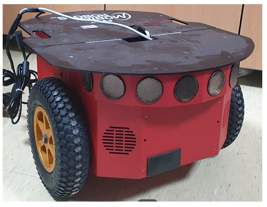
3.2. Mobile Robot
3.3. Laser Range Finder (LRF)
4. Environment Map Generation Algorithm in a Transparent Obstacle Environment
- Transparent obstacles are in the form of a straight line.
- No opaque obstacle exists adjacent to the transparent obstacle that is on the opposite side of the LRF.
- All obstacles are fixed in their positions, and they are not known.
| Algorithm 1. Pseudo code of the algorithm used to create environment maps for environments with transparent obstacles. |
| Input: |
| (t) ← Distance towards the direction (t) measured at time t |
| (t) ← Angle value of nth sensor beam measured at time t |
| (t) ← Position (x, y) of the robot at time t |
| (t) ← Direction that robot is heading towards at time t |
| Output: |
| SDCMap ← Global map representing the accumulated number of detected sensor beams in a certain cell to decide obstacle cell |
| Begin Algorithm Creating Environment maps with Transparent Obstacle |
| 1 For (t) in all sensor beams n: {1 ~ 1081} do |
| 2 If ≤ (t) ≤ then |
| 3 (t) ← f((t),(t),(t),(t)) |
| 4 Else |
| 5 (t) ← −1 |
| 6 If (t) == (t) then |
| 7 WDCMap((t)) += 1 |
| 8 Else If (t−1) ≠ (t) then |
| 9 If WDCMap((t)) ≥ then |
| 10 SDCMap((t)) += g(WDCMap((t))) |
| 11 Else If WDCMap((t)) ≥ Or (t) ∈ ((t−1)) then |
| 12 L ← Rasterization((t),(t)) |
| // L: The list of cells included in the virtual line segment |
| // connecting L[0]: (t) and L[NUM_CELLS]: (t) |
| 13 ← Find_NearCell((t), L) // Function finding the closest but not the |
| // same cell from (t) in the list L |
| 14 loop: |
| 15 SDCMap ← DetectObstacleCandidate(, L, NUM_CELLS) |
| 16 Goto loop |
| 17 If there is no in L s.t. SDCMap () > 0 then |
| 18 SDCMap((t)) += 1 |
| 19 Else |
| 20 If (t) ∈ (t) then |
| 21 SDCMap((t)) += 1 |
| 22 Else |
| 23 Append (t) to (t) |
| 24 WDCMap((t)) ← 0 |
| End Algorithm Creating Environment maps with Transparent Obstacle |
| Algorithm 2. Pseudo code of the algorithm used to DetectObstacleCandidate(). |
| Input: |
| ← Result of function finding the closest but not the same cell from (t) in the list L |
| L ← List of cells included in the virtual line segment |
| NUM_CELLS ← Last index number of list L |
| Output: |
| SDCMap ← The global map representing the accumulated number of detected sensor beams in a certain cell to decide obstacle cell |
| Begin Algorithm Detect Obstacle Candidate |
| 1 If SDCMap() > 0 then |
| 2 If WDCMap(L[NUM_CELLS]) ≥ then // L[NUM_CELLS]: (t) |
| 3 SDCMap() += g(WDCMap(L[NUM_CELLS])) |
| 4 Else |
| 5 SDCMap() += 1 |
| 6 INIT_CELL ← 1 |
| 7 ← Find_NearCell(, L[INIT_CELL:NUM_CELLS]) |
| // Function finding the closest but not the same cell from L[0] == in the list L |
| 8 loop: |
| 9 If WDCMap((t)) ≥ then |
| 10 SDCMap() -= g(WDCMap((t))) |
| 11 Else |
| 12 SDCMap() −= 1 |
| 13 INIT_CELL += 1 // INIT_CELL: 1, 2, … , NUM_CELLS |
| 14 ← Find_NearCell(, L[INIT_CELL:NUM_CELLS]) |
| 15 Goto loop |
| 16 L ← L–{} // Update L With the reduced size |
| 17 ← Find_NearCell(, L[INIT_CELL:NUM_CELLS-1]) |
| End Algorithm Detect Obstacle Candidate |
- The cell containing transparent obstacles have higher WDCMap compared to a cell detected by irregular noise due to the regularity of the reflection noise generated by transparent obstacles. Although the value of the WDCMap((t)) is not higher than , if it is higher than the value of , it is marked as a candidate of transparent obstacle.
- While the robot is moving, the reflection noise occurs continuously, but common noises occur intermittently by opaque obstacles and the surrounding environment. Using this property, it is considered as a candidate for a transparent obstacle if the (t) at time t correspond to any of ((t−1)) at time t.
- The reflection noise generated by transparent obstacles may contain a cell that has low WDCMap because it is not detected continuously; however, if it is detected regularly, it is considered to be a candidate for a transparent obstacle.
5. Path Planning in an Environment with Transparent Obstacles
- A path planning method that can be applied to the occupancy grid map must be used.
- A new path must be generated quickly within the environment map being updated by the sensor data being collected in real time.
- The generated path should be close to the optimized one.
| Algorithm 3. Pseudo code for the Wavefront-propagation algorithm [24]. (Citation mark) |
| BeginAlgorithm Wavefront-propagation |
| 1 Initialize ← , i ← 0 |
| 2 Initialize ← |
| 3 For every x ∈ , assign (x) = i and insert All unexplored neighbors of x do |
| 4 If == then |
| 5 Terminate |
| 6 Else |
| 7 i ← i + 1 |
| 8 Goto step 2 |
| EndAlgorithm Wavefront-propagation |
6. Experimental Results
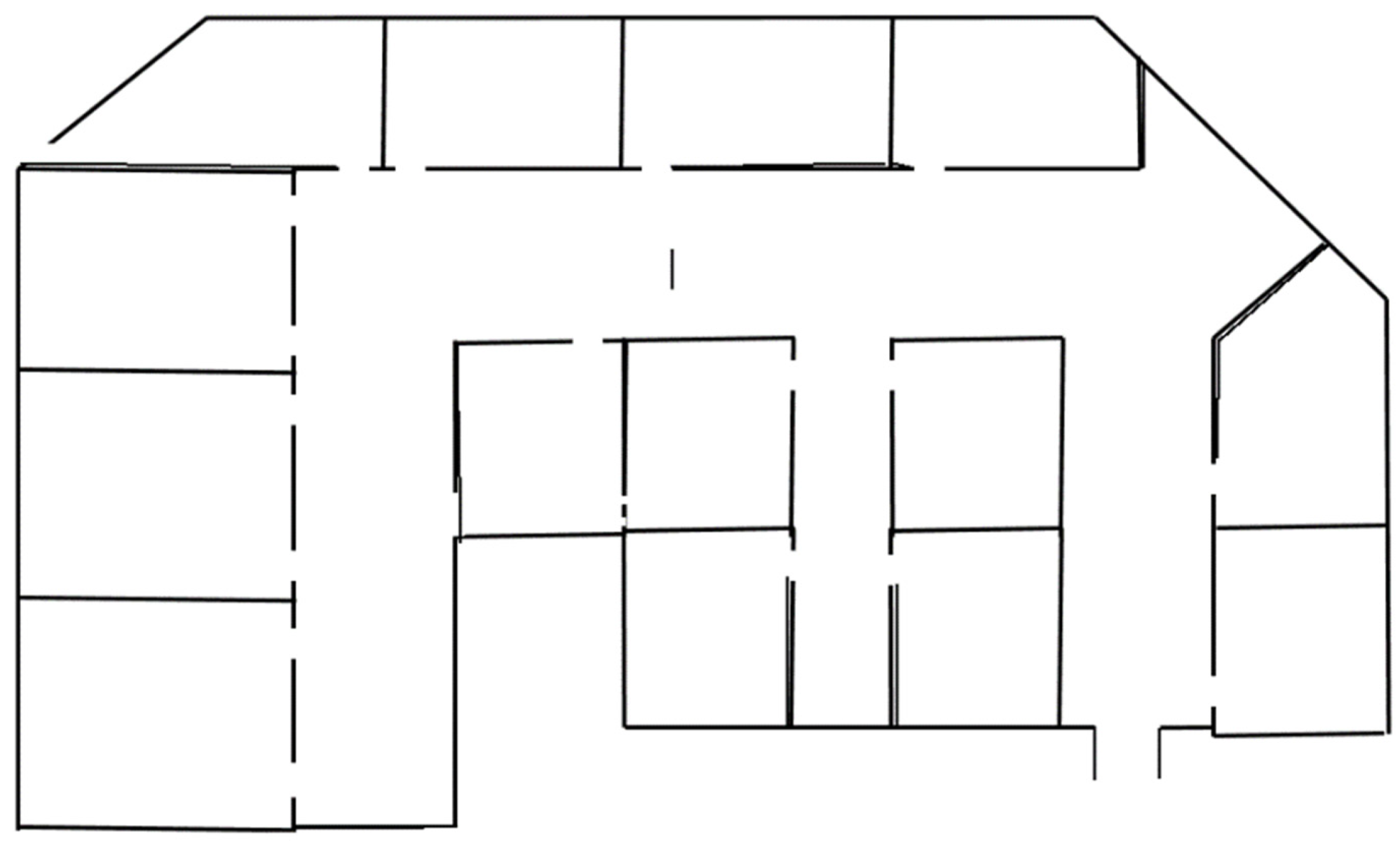
6.1. Experimental Environment
6.2. Environment Map Generation Experiment in an Environment with Transparent Obstacles
6.2.1. Experimental Method
- The robot drove alongside the wall of transparent obstacles with a 30 cm distance away from it.
- The robot drove towards the wall in a direction angled 45 degrees at a position far from the wall of the transparent obstacle, and the robot’s position moved parallel to the wall once it reached 30 cm distance away from the wall.
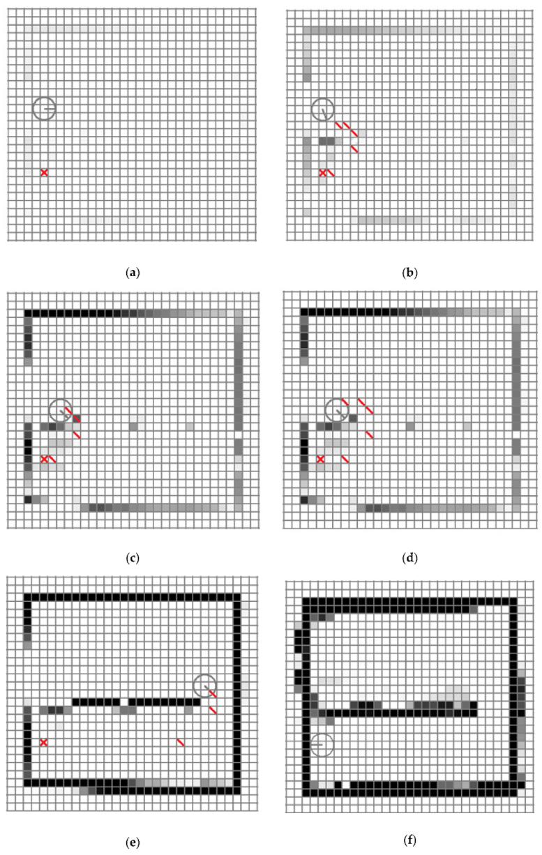
6.2.2. Analyses of the Experimental Results
6.3. Mobile Robot Path Planning Experiment in an Environment with Transparent Obstacles
6.3.1. Experimental Method
6.3.2. Experiment Result Analysis
6.4. Error Rate Experiment
Experimental Method
7. Conclusions
Author Contributions
Funding
Conflicts of Interest
References
- Tsubouch, T. Nowadays trend in map generation for mobile robots. In Proceedings of the IEEE International Conference on Intelligent Robot and System, Osaka, Japan, 8 November 1996; Volume 2, pp. 828–833. [Google Scholar]
- Moravec, H.P.; Elfes, A.E. High resolution maps from wide angle sonar. In Proceedings of the IEEE International Conference on Robotics and Automation, St. Louis, MO, USA, 25–28 March 1985; Volume 2, pp. 116–121. [Google Scholar]
- Leonard, J.J.; Durant-Whyte, H.F. Dynamic Map Building for an Autonomous Mobile Robot. Int. J. Robot. Res. 1992, 11, 286–298. [Google Scholar] [CrossRef]
- Stateczny, A.; Kazimierski, W.; Gronaska-Siedz, D.; Motly, W. The Empirical Application of Automotive 3D Rader Sensor for Target Detection for an Autonomous Surface Vehicle’s Navigation. Remote Sens. 2019, 11, 1156. [Google Scholar] [CrossRef]
- Jung, J.-W.; So, B.-C.; Kang, J.-G.; Lim, D.-W.; Son, Y. Expanded Douglas–Peucker Polygonal Approximation and Opposite Angle-Based Exact Cell Decomposition for Path Planning with Curvilinear Obstacles. Appl. Sci. 2019, 9, 638. [Google Scholar] [CrossRef]
- Feder, H.J.S.; Leonard, J.J.; Smith, C.M. Adaptive mobile robot navigation and mapping. Int. J. Robot. Res. 1999, 18, 650–668. [Google Scholar] [CrossRef]
- Park, J.-S.; Jung, J.-W. Transparent Obstacle Detection Method based on Laser Range Finder. J. Korean Inst. Intell. Syst. 2014, 24, 111–116. [Google Scholar] [CrossRef][Green Version]
- Jensgelt, P. Approaches to Mobile Robot Localization in Indoor Environments. Ph.D. Thesis, KTH Royal Institute of Technology, Stockholm, Sweden, 2001. [Google Scholar]
- Zhuang, Y.; Sun, Y.; Wang, W. Mobile Robot Hybrid Path Planning in an Obstacle-Cluttered Environment Based on Steering Control and Improved Distance Propagation. Int. J. Innov. Comput. Inf. Control 2012, 8, 4098–4109. [Google Scholar]
- Sohn, H.-J. Vector-Based Localization and Map Building for Mobile Robots Using Laser Range Finder in an indoor Environments. Ph.D. Thesis, Korea Advanced Institute of Science and Technology (KAIST), Daejeon, Korea, 2008. [Google Scholar]
- Jung, Y.-H. Development of a Navigation Control Algorithm for Mobile Robot Using D* Search Algorithm. Master’s Thesis, Chungnam University, Daejeon, Korea, 2008. [Google Scholar]
- Park, J.-S.; Jung, J.-W. A method to LRF noise Filtering for the transparent obstacle in mobile robot indoor navigation environment with straight glass wall. In Proceedings of the IEEE International conference on Ubiquitous Robots and Ambient Intelligence, Xi’an, China, 19–22 August 2016; pp. 194–197. [Google Scholar]
- Koenig, S. Fast Replanning for Navigation in Unknown Terrain. IEEE Trans. Robot. 2005, 21, 354–363. [Google Scholar] [CrossRef]
- Guo, J.; Liu, Q.; Qu, Y. An improvement of D* Algorithm for Mobile Robot Path Planning in Partial Unknown Environments. Intell. Comput. Technol. Automob. 2009, 3, 394–397. [Google Scholar]
- Kuipers, B.; Byum, Y.T. A robot exploration and mapping strategy based on a semantic hierarchy of spatial representations. Robot. Auton. Syst. 1991, 8, 47–63. [Google Scholar] [CrossRef]
- Choset, H.; Burdick, J. Sensor-Based exploration: The hierarchy generalized voronoi graph. Int. Robot. Res. 2000, 19, 96–125. [Google Scholar] [CrossRef]
- Young, D.K.; Jin, S.L. A Stochastic Map Building Method for Mobile Robot using 2D Laser Range Finder. Auton. Robot 1999, 7, 187–200. [Google Scholar]
- Rudanm, J.; Tuza, G.; Szederkenyi, G. Using LMS-100 Laser Range Finder for indoor Metric Map Building. In Proceedings of the 2010 IEEE International Symposium on Industrial Electronics, Bari, Italy, 4–7 July 2010; pp. 520–530. [Google Scholar]
- Jung, J.-H.; Kim, D.-H. Local Path Planning of a Mobile Robot Using a Novel Grid-Based Potential Method. Int. J. Fuzzy Log. Intell. Syst. 2020, 20, 26–34. [Google Scholar] [CrossRef]
- Siciliano, B.; Khatib, O. Handbook of Robotics; Springer: Berlin, Germany, 2008. [Google Scholar]
- Latombe, J. Robot Motion Planning; Kluwer Academic Publisher: Cambridge, MA, USA, 1991. [Google Scholar]
- Nohara, Y.; Hasegawa, T.; Murakami, K. Floor Sensing System using Laser Range Finder and Mirror for Localizing Daily Life Commodities. In Proceedings of the IEEE/RSJ International Conference on Intelligent Robots and Systems, Taipei, Taiwan, 18–22 October 2010; pp. 1030–1035. [Google Scholar]
- Choset, H.; Lynch, K.M.; Hutchinson, S.; Kantor, G.; Burgard, W.; Kavaraki, L.E.; Thrum, S. Principles of Robot Motion: Theory, Algorithm and Implementation; MIT Press: Cambridge, MA, USA, 2005. [Google Scholar]
- La Valle, S.M. Planning Algorithms; Cambridge University Press: Cambridge, MA, USA, 2006. [Google Scholar]
- Stentz, A. Optimal and Efficient Path Planning for Partially-Known Environments. In Proceedings of the IEEE International Conference on Robotics and Automation, San Diego, CA, USA, 8–13 May 1994; Volume 4, pp. 3310–3317. [Google Scholar]
- Siegwart, R.; Nourbakhsh, I.R. Introduction to Autonomous Mobile Robot; MIT Press: Cambridge, MA, USA, 2004. [Google Scholar]
- Willms, A.R.; Yang, S.X. An Efficient Dynamic System for Real-Time Robot—Path Planning. IEEE Trans. Syst. Cybern. Part B Cybern. 2006, 36, 755–766. [Google Scholar] [CrossRef] [PubMed]
- Nguyen Van, V.; Kim, Y.-T. An Advanced Motion Planning Algorithm for the Multi Transportation Mobile Robot. Int. J. Fuzzy Log. Intell. Syst. 2019, 19, 67–77. [Google Scholar]
- Mingxiu, L.; Kai, Y.; Chengzhi, S.; Yutong, W. Path Planning of Mobile Robot Based on Improved A* Algorithm. In Proceedings of the IEEE 29th Chinese Control and Decision Conference (CCDC), Chongqing, China, 28–30 May 2017. [Google Scholar]
- Rui, S.; Yuanchang, L.; Richard, B. Smoothed A* Algorithm for Practical Unmanned Surface Vehicle Path Planning. Appl. Ocean Res. 2019, 83, 9–20. [Google Scholar]
- Guo-Hua, C.; Jun-Yi, W.; Ai-Jun, Z. Transparent object detection and location based on RGB-D Camera. J. Phys. Conf. Ser. 2019, 1183, 012011. [Google Scholar] [CrossRef]
- Cui, C.; Graber, S.; Watson, J.J.; Wilcox, S.M. Detection of Transparent Elements Using Specular Reflection. U.S. Patent 10,281,916, 7 May 2019. [Google Scholar]
- Pioneer Corporation. Available online: https://www.pioneerelectronics.com/ (accessed on 16 April 2020).
- SICK Sensor Intelligence. Available online: https://www.sick.com/ (accessed on 16 April 2020).
- Lumelsky, V.; Skewis, T. Incorporation Range Sensing in The Robot. IEEE Trans. Syst. 1990, 20, 1058–1068. [Google Scholar]
- Moravec, H.P. Sensor fusion in certainty grids for mobiles robots. Ai Mag. 1988, 9, 61–74. [Google Scholar]


| Terminology | Explanation |
|---|---|
| (t) | The angle value of nth sensor beam measured at time t (t) = +*(n-1), n:1 ~ 1081, = -45(deg), = 0.25(deg) |
| (t) | The distance towards the direction (t) measured at time t |
| The minimum distance that sensor can recognize: 50 cm | |
| The maximum distance that sensor can recognize: 20 m | |
| (t) | The position (x, y) of the robot at time t |
| (t) | The direction that robot is heading towards at time t |
| f((t),(t),(t),(t)) | The position of the cell located from (t) with the distance (t) and the heading angle (t) + (t) (Represented as cell No.) |
| (t) | The position of the cell on the grid map calculated using f((t),(t),(t),(t)) at time t (Represented as cell No.) |
| (t) | The position of the robot center point on the grid map at time t (represented as cell No.) |
| WDCMap(cell) | The temporary local map representing the number of detected sensor beams in a certain cell (weakly detected counter (WDC) map) |
| SDCMap(cell) | The global map representing the accumulated number of detected sensor beams in a certain cell to decide obstacle cell (strongly detected counter (SDC) map) |
| (t) | The set of cells with WDCMap(cell) = 0 at time t |
| ((t−1)) | The set of cells pointed by n-1-rth, ∙∙∙ , n-1-1th, n-1th, n-1+1th, ∙∙∙ , n-1+rth beams at time t-1 (default value: r = 1) |
| g(x) | A function emphasizing the extent of increase of the SDCMap(cell) (default function: g(x) = x) |
| The threshold number of WDC to determine opaque obstacle (default value = 5, WDC = weakly detected counter) | |
| The threshold number of WDC to determine the transparent obstacle candidate (default value = 1, ) | |
| The threshold number of WDC to determine the surface of transparent obstacle (default value = 3) |
| Terminology | Explanation |
|---|---|
| The cost required to propagate Wavefront | |
| The set of cells for ith propagation | |
| The set of cells in which the destination is stored (default: The number of destination cells is 1) | |
| (x) | The function to store the optimized propagation cost of cells that belong to |
| All unexplored neighbors of x | The non-obstacle cells not yet propagated among adjacent cells with four different directions |
| Environment 1 | Environment 2 | Environment 3 | |
|---|---|---|---|
| Using only data from LRF | 12.26 | 19.57 | 21.40 |
| Using LRF and the algorithm | 6.45 | 7.20 | 4.73 |
© 2020 by the authors. Licensee MDPI, Basel, Switzerland. This article is an open access article distributed under the terms and conditions of the Creative Commons Attribution (CC BY) license (http://creativecommons.org/licenses/by/4.0/).
Share and Cite
Jung, J.-W.; Park, J.-S.; Kang, T.-W.; Kang, J.-G.; Kang, H.-W. Mobile Robot Path Planning Using a Laser Range Finder for Environments with Transparent Obstacles. Appl. Sci. 2020, 10, 2799. https://doi.org/10.3390/app10082799
Jung J-W, Park J-S, Kang T-W, Kang J-G, Kang H-W. Mobile Robot Path Planning Using a Laser Range Finder for Environments with Transparent Obstacles. Applied Sciences. 2020; 10(8):2799. https://doi.org/10.3390/app10082799
Chicago/Turabian StyleJung, Jin-Woo, Jung-Soo Park, Tae-Won Kang, Jin-Gu Kang, and Hyun-Wook Kang. 2020. "Mobile Robot Path Planning Using a Laser Range Finder for Environments with Transparent Obstacles" Applied Sciences 10, no. 8: 2799. https://doi.org/10.3390/app10082799
APA StyleJung, J.-W., Park, J.-S., Kang, T.-W., Kang, J.-G., & Kang, H.-W. (2020). Mobile Robot Path Planning Using a Laser Range Finder for Environments with Transparent Obstacles. Applied Sciences, 10(8), 2799. https://doi.org/10.3390/app10082799