Minimal Model for Sprag-Slip Oscillation as Catastrophe-Type Behavior

Abstract

The infinite spragging force can be produced by a spring inclined with a constant angle in a frictional sliding system. The ensuing oscillation is called the sprag-slip oscillation. This sprag-slip oscillation is re-examined by using the minimal nonlinear dynamic model with the variable angle of the inclined spring. Nonlinear equilibrium equation is converted into the novel polynomial form. This simple but more realistic sprag model shows that the infinite spragging force is not realistic and the catastrophic static deformation in the steady-sliding state can occur. It indicates that the ‘sprag’, termed by Spurr, can be described by this catastrophic characteristic of the frictional sliding system.

1. Introduction

Friction-induced vibration is usually known as self-excited vibration by friction producing unwanted phenomena such as vibration, noise, and fatigue. Owing to its frequent and serious problems in many applications such as automotive brakes, machine joints, and tools, enormous research for the source of instability in the friction-engaged system has been conducted over the decades [1,2,3,4,5,6,7,8,9,10,11,12,13,14,15,16,17].

In the literature, the minimal model has been widely used to explain the dynamic instability induced by the negative friction-slope and mode-coupling instability [10,11,12,13]. In a general approach, a stability analysis based on linear eigenvalue analysis was performed and stability boundaries in the parameter space were derived for the equilibrium of the system. Then, their nonlinear stick-slip oscillations at the unstable steady-sliding equilibrium have been demonstrated by solving discontinuous differential equations using several different friction models such as the smoothing [10] and switching [11] methods.

In this scenario, the determination of the dynamic instability in the parameter space is valid when steady-sliding exists, and the resulting nonlinear motion in this space can be reasonably found. However, in the parameter space for which steady-sliding does not exist, the above analysis is no more applicable, and the true nonlinear response cannot be examined. Therefore, the determination of the parameter space for which the steady-sliding does not exist is critical for the so-called “sprag-slip oscillation”.

Sprag-type instability and its realistic interpretation were of particular interest in this study. Its dynamic behavior has not been vigorously investigated due to its unbounded and discontinuous nature. The term “sprag” was firstly named by Spurr in his article [1] by using two simple examples: One, the inclined rigid rod hinged at one end under sliding and can have infinite contact forces, and two, the mass attached by an inclined spring and may experience an unbounded steady-sliding equilibrium (equivalent to the infinite contact forces) for a certain geometric condition. Later, this kinematic constrained instability was investigated in the beam-on-disk system by Jarvis et al. [14] and the pin-disc model by Earles et al. [15]. In the beam-on-belt configuration, Hoffmann et al. [16] extended the sprag theory by assuming that the sprag condition can be, in another way, characterized as the non-existence of the steady-sliding equilibrium, which is presumably equivalent to the lift-off of the sliding beam at the contact. Kang et al. [17] also investigated the sprag conditions of the several sliding mass-spring systems and found that, in the parametric space, the unbounded spragging force corresponds to the boundary of the regime for the non-existence of the steady-sliding equilibrium. In other words, the sprag condition in [1] is shown to be the condition for the onset of loss-of-contact in [16,17]. However, it is still unclear that the sprag-type oscillation truly exists in the friction-sliding system. The infinite contact force or the loss of contact at sliding is quite ambiguous from the engineering point of view. Honestly, the sprag-slip oscillation is not based on the mathematical principles, but the hypothesis that a lacking steady-sliding presumably leads to stick-slip oscillation.

The infinite contact force is generated in a specific region in the parametric space by a linearized equilibrium. [17] Kinematic and dynamic analysis includes initial condition and static equilibrium position in open and closed loop mechanisms. Hence, it is very important to find the equilibrium position. In dynamical system, steady-sliding equilibrium can be represented by a nonlinear equation. Its nonlinear equation derives a solution with abrupt changes that are difficult to predict in a parametric space. Nonlinearities, such as social and behavioral sciences and natural phenomena where continuous changes in parameters can lead to discontinuous changes in the resulting variables, are described as cusp catastrophes [18,19,20,21,22,23,24,25,26,27,28].

Qin et al. [19] studied the necessary and sufficient conditions leading to landslides. The bifurcation point is a turning point from stability to potential instability, showing that chaos can be formed. It also shows that the chaos phenomenon is related to the mechanical parameters of the medium along the sliding surface. In a similar study case, Miao et al. [23] studied the dynamical behavior of water or gas flow in a broken rock. They used the catastrophe theory to obtain the fold catastrophe model of the stability of flow system and predicted that dynamic disasters could occur near bifurcation. In this way, the catastrophe theory was used to analyze bifurcation curve in a nonlinear equilibrium. In another study, cusp catastrophe interpretation was also studied in the analysis of dynamic instability due to friction. Carpinteri et al. [24] simulated the problem of tangential force with the perspective of a micromechanical contact model. It has also been shown that reducing the applied normal force results in energy release due to snap-back instability associated with tangential force and sliding displacement. This result provides an explanation of the stick-slip phenomenon according to the catastrophe theory of tangential load, which showed similar to cusp-catastrophe instability. Tian et al. [28] expressed equilibrium surfaces using cusp catastrophe theory in harmful algae blooms (HABs). The static equilibrium surface consists of two stable areas and a folded area, which can be projected as a bifurcation set. When entering the bifurcation set on the equilibrium surface, the state variable suddenly jumps and causes cusp catastrophes of the system.

The basic concept of the cusp catastrophe theory is the ’potential’ of the system, and it tends to produce certain sudden results. Catastrophic phenomena undergo periods of equilibrium at a minimum potential and, conversely, periods of sudden changes at a maximum potential. The potential of the system is not a structurally stable function, but the critical point (singularity) is degenerated.

In the field of multi-body dynamics, the nonexistence of solutions under the Coulomb friction on rigid contact is well known as Painleve’s paradox [29,30,31,32,33]. Under the assumption of the impenetrability where the gap between the rigid system and rigid ground is not allowed negative, the occurrence of inconsistency and indeterminate can be found in the parameter space. Frictional hopping motion has been suggested as the similar kind of sprag-slip oscillation by the Painleve paradox [29]. Painleve’s paradox was well introduced in a review study by Champneys et al. [33]. The author described the Painleve’s paradox through the difference between pulling and pushing force by inducing chalk’s sprag-slip vibration. In addition, various minimal models were reinterpreted to describe the uncertainty, multiple stability, and instability associated with Painleve’s paradox. In compliant contact for which the negative gap is allowed, the indeterminate of the steady-sliding equilibrium was found in the parameter space [16,17].

However, the static and dynamic phenomenon at a nonlinear equilibrium of a dynamic system has not been investigated when a sudden jump occurs in friction-induced vibration. The previous study [17] presumed that the so-called “sprag-slip oscillation” occurs when a singular condition such as no steady-sliding situation is met. The purpose of the present work was to resolve this singularity problem and explain the sprag-slip oscillation in a continuous manner. For this, the more and realistic nonlinear modeling was introduced and adopted.

In our model, one mass was attached by an inclined spring where the inclined spring angle was allowed varying. This simple and nonlinear configuration was the key avoiding the paradoxical case mentioned above. It resulted in the fully nonlinear equations of equilibrium, which seemed very complicated to solve. However, we successfully converted them into the novel polynomial form to be analytically solved. The solution set of the equilibrium equations will be used to show how the non-existence of steady-sliding was avoided and bifurcation set was formed in the parametric space. Then, the sprag phenomenon, understood as the infinite spragging force, was newly interpreted as the catastrophe-type behavior with finite static sliding deformation.

2. Materials and Methods

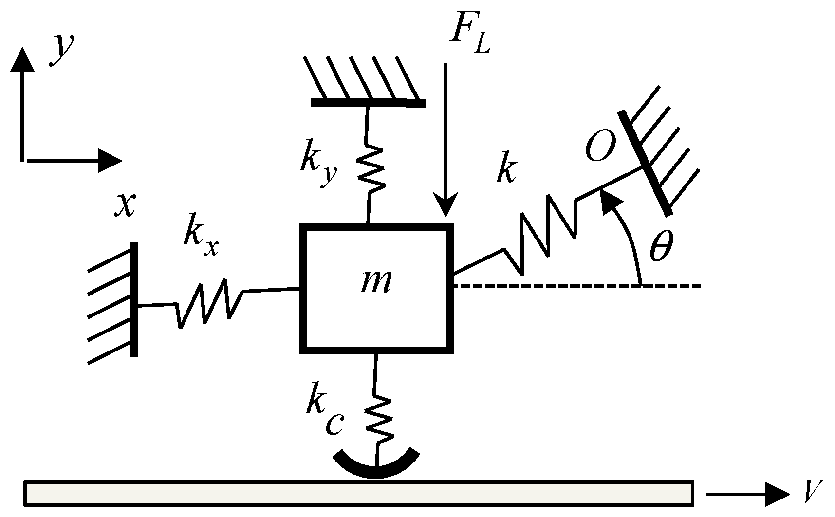
A simple compliant model was proposed, as shown in Figure 1. The $k_x$ and $k_y$ represent system stiffness fixed to ground as opposed that the inclined stiffness and $k$ was applied for representing kinematic variation of system stiffness during sliding. The contact stiffness $k_c$ was applied for allowing the downward acceleration. It should be noted that the inclined stiffness $k$ may produce the infinite spragging force for the constant inclined angle [17]. In the present work, the inclined angle $\theta$ was allowed varying for preventing the sprag force from becoming infinite and providing the nonlinear perspective on spragging, as shown in Figure 2.

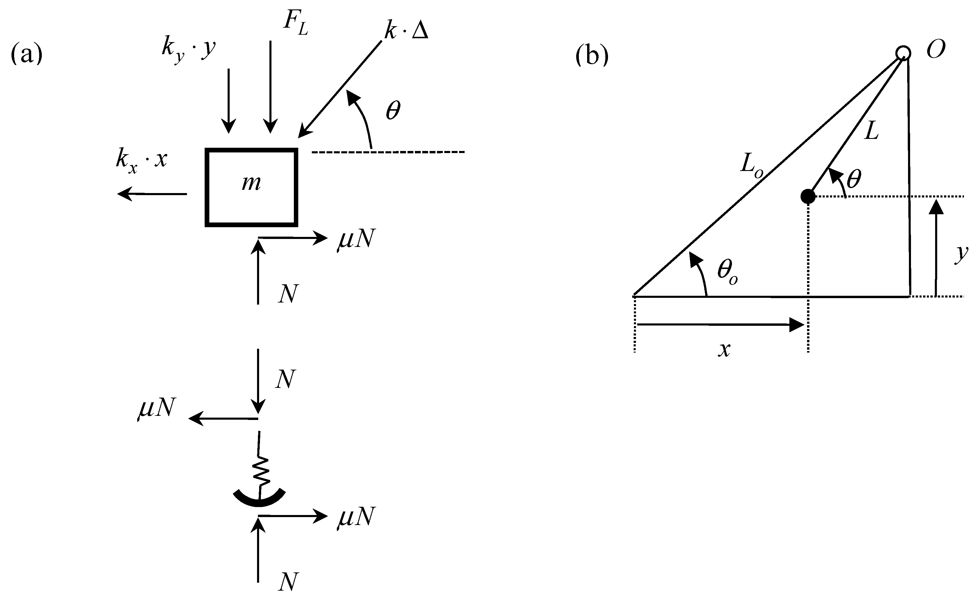
The equations of motion for this nonlinear spring-mass model are given by:

$$m\ddot{x}=\mu N-k\Delta \cos \theta -k_{x}x$$

(1)

$$m\ddot{y}=N-F_L-k\Delta \sin \theta -k_{y}y$$

(2)

where the stretch/compression in the inclined spring is obtained from (Figure 2b):

$$\Delta =L_o-L$$

(3)

and where the relationship between the original length $L_o$ and the deformed length $L$ is given by:

$$L\cos \theta =L_o\cos {\theta }_o-x$$

(4)

$$L\sin \theta =L_o\sin {\theta }_o-y$$

(5)

$$L=\sqrt{{\left(L_o\cos \theta -x\right)}^2+{\left(L_o\sin \theta -y\right)}^2}$$

(6)

It is important to note that the contact normal load $N$ in Equations (1) and (2) is a nonsmooth function defined as:

$$N=\{\begin{array}{c}-k_{c}y,\begin{array}{c}\end{array}if\begin{array}{c}\end{array} y<0\\ 0,\begin{array}{c}\end{array}if\begin{array}{c}\end{array} y\ge 0\end{array}$$

(7)

The equations of motion, Equations (1)–(2), can be rewritten in the dimensionless form by introducing the new time scale and system parameters:

$$x^{″}+\frac{\sigma }{L}\left(1-L\right)\left(\cos {\theta }_o-x\right)+\alpha x-\mu n=0$$

(8)

$$y^{″}+\frac{\sigma }{L}\left(1-L\right)\left(\sin {\theta }_o-y\right)+\beta y-n=0$$

(9)

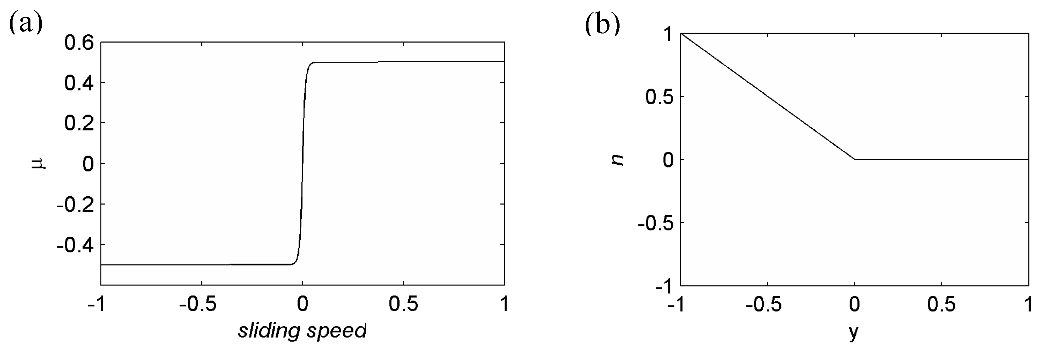
where $\tau =t\sqrt{k_c/m}$, ${(•)}^{\prime }=d(•)/d\tau$, $x\to x/L_o$, $y\to y/L_o$, $L\to L/L_o$, $\sigma =k/k_c$, $\alpha =k_x/k_c$, $\beta =k_y/k_c$, $\kappa =F_L/\left(k_c{L}_o\right)$, and $n=N/k_c$. For a convenient mathematical form, $\mu$ is set to be a regularized friction coefficient and $n$ is expressed in a mathematical function form such that:

$$\mu ={\mu }_o\left\{1-\exp \left(-d\left|V-\dot{x}\right|\right)\right\}sgn(V-\dot{x})$$

(10)

$$n=\frac{1}{2}\left(\left|y\right|-y\right)$$

(11)

where $d$ is the control parameter in the creep regime (Figure 3).

The system equilibriums can be found from Equations (8) and (9) when $x^{″}=x^{\prime }=0$ and $y^{″}=y^{\prime }=0$. The corresponding equilibrium equations become:

$$F_x=\frac{\sigma }{L}\left(1-L\right)\left(\cos {\theta }_o-x\right)+\alpha x-{\mu }_{o}n=0$$

(12)

$$F_y=\frac{\sigma }{L}\left(1-L\right)\left(\sin {\theta }_o-y\right)+\beta y-n=0$$

(13)

Here the two set of equilibrium equations are formulated for the contact and noncontact conditions. For the contact condition, $n>0$, the equilibrium equations are rewritten as:

$$\sigma \left(1-L\right)\cos \theta +\alpha \left(\cos {\theta }_o-L\cos \theta \right)+{\mu }_o\left(\sin {\theta }_o-L\sin \theta \right)=0$$

(14)

$$\sigma \left(1-L\right)\sin \theta +\beta \left(\sin {\theta }_o-L\sin \theta \right)+\left(\sin {\theta }_o-L\sin \theta \right)=-\kappa$$

(15)

It can be also expressed in the matrix form:

$$D\left\{\begin{array}{c}\cos \theta \\ \sin \theta \end{array}\right\}=b$$

(16)

where

$$D=\sigma I+LA$$

(17)

$$A=\left[\begin{array}{cc}-\left(\sigma +\alpha \right)& -\mu \\ 0& -\left(\sigma +\beta +1\right)\end{array}\right]$$

(18)

$$b=\left\{\begin{array}{c}-\alpha \cos {\theta }_o-\mu \sin {\theta }_o\\ -\left(\beta +1\right)\sin {\theta }_o-\kappa \end{array}\right\}$$

(19)

For further numerical calculation, Equation (16) is converted into:

$${\left\{\begin{array}{c}\cos \theta \\ \sin \theta \end{array}\right\}}^T\left\{\begin{array}{c}\cos \theta \\ \sin \theta \end{array}\right\}=1=b^T{\left(D{D}^T\right)}^{-1}b$$

(20)

which results in the polynomial equations in $L$:

$$c_0+c_{1}L+c_2{L}^2+c_3{L}^3+c_4{L}^4=0$$

(21)

where the coefficients are referred to in the Appendix A. The solutions of Equation (21) give the steady-sliding equilibriums.

Similarly, for the noncontact condition, $n=0$, the equilibrium equations are expressed in the matrix form:

$$\tilde{\mathbf{D}}\left\{\begin{array}{c}\cos \theta \\ \sin \theta \end{array}\right\}=\tilde{\mathbf{b}}$$

(22)

$${\left\{\begin{array}{c}\cos \theta \\ \sin \theta \end{array}\right\}}^T\left\{\begin{array}{c}\cos \theta \\ \sin \theta \end{array}\right\}=1={\tilde{\mathbf{b}}}^T{\left(\tilde{\mathbf{D}}{\tilde{\mathbf{D}}}^T\right)}^{-1}\tilde{\mathbf{b}}$$

(23)

where

$$\tilde{\mathbf{D}}=\left[\begin{array}{cc}\sigma \left(1-L\right)-L\alpha & 0\\ 0& \sigma \left(1-L\right)-L\beta \end{array}\right]$$

(24)

$$\tilde{\mathbf{b}}=\left\{\begin{array}{c}-\alpha \cos {\theta }_o\\ -\beta \sin {\theta }_o-\kappa \end{array}\right\}$$

(25)

The corresponding polynomial equation in $L$ is given by:

$$d_0+d_{1}L+d_2{L}^2+d_3{L}^3+d_4{L}^4=0$$

(26)

where its coefficients are also referred to in the Appendix A. The solutions of Equation (26) represent the equilibriums under the noncontact condition. Therefore, the possible equilibriums of this nonlinear spring-mass model can be either the steady-sliding equilibriums or the static equilibrium without contact.

The stability of the equilibrium is determined by the eigenvalue $\lambda$ of Equations (12) and (13):

$$\det \left({\lambda }^{2}I+K\right)=0$$

(27)

where

$$K={\left[\begin{array}{cc}\frac{\partial F_x}{\partial x}& \frac{\partial F_x}{\partial y}\\ \frac{\partial F_y}{\partial x}& \frac{\partial F_y}{\partial y}\end{array}\right]}_{equilibriums}=\left[\begin{array}{cc}\sigma \left(1-\frac{{\sin }^2{\theta }_{eq}}{L_{eq}}\right)+\alpha & \frac{\sigma }{L_{eq}}\sin {\theta }_{eq}\cos {\theta }_{eq}+{\mu }_o\overline{n}\\ \frac{\sigma }{L_{eq}}\sin {\theta }_{eq}\cos {\theta }_{eq}& \sigma \left(1-\frac{{\cos }^2{\theta }_{eq}}{L_{eq}}\right)+\beta +\overline{n}\end{array}\right]$$

(28)

where

$$\overline{n}=\{\begin{array}{c}1\begin{array}{c},\end{array}\begin{array}{c}\end{array}\begin{array}{c}if\begin{array}{c}\end{array} n\ne 0\end{array}\\ 0\begin{array}{c},\end{array}\begin{array}{c}\end{array}\begin{array}{c}if\begin{array}{c}\end{array} n=0\end{array}\end{array}$$

(29)

3. Results

For the preliminary investigation, ${\theta }_o$ was chosen to be a control parameter and the other system parameters were set to be ${\mu }_o=0.5$, $\kappa =0.007$, $\alpha =0.007$, $\sigma =0.1$, and $\beta =0$ for clearly showing the catastrophic behavior. The equilibrium curve and its stability types can be determined by solving Equations (21), (22), and (27) numerically with respect to ${\theta }_o$. The equilibrium set of the contact and noncontact conditions can be obtained separately, as shown in Figure 4a,b and Figure 4c,d, respectively. The fixed points under contact ($y_{eq}<0$) are the steady-sliding equilibriums essential in the friction-induced vibration problems. However, the fixed points under noncontact condition ($y_{eq}\ge 0$) represent the static equilibrium in the lift-off state that was not of interest in this analysis. The dynamic behavior of the system can be investigated by the stability at the sliding deformation with respect to the control parameter, as illustrated in Figure 4a. In this example, three steady-sliding equilibriums exist for the lower and upper range of ${\theta }_o$ where one is geometrically unstable and the others are stable.

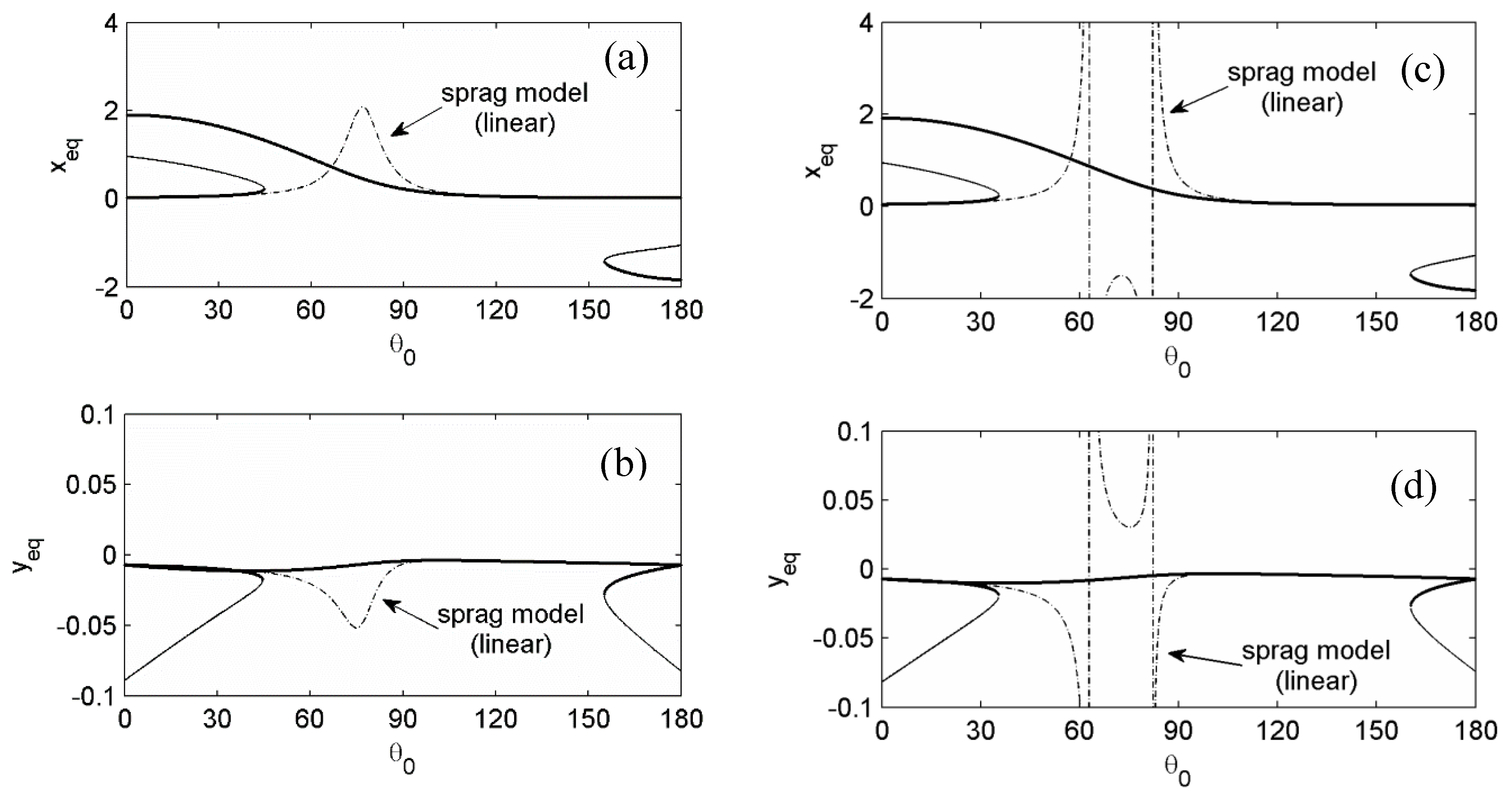
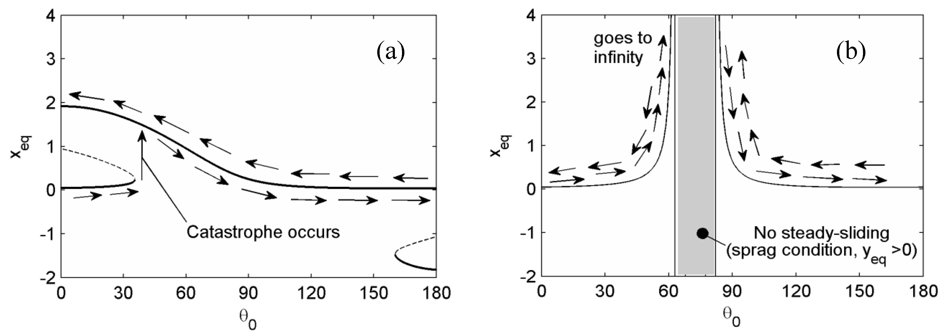
It is important to note that, for the constant inclined angle case [17], the steady-sliding disappeared under the so-called sprag condition. This constant angle approximation will be called the "linear sprag model". The corresponding dynamic behavior can be hardly analyzed due to its discontinuous characteristics. Therefore, the spragging force should be interpreted by the proposed nonlinear model.

In this example, the critical value for the existence of the sprag condition in the linear sprag model was around ${\mu }_o\equiv {\mu }_{cr}=0.58$. The steady-sliding equilibrium of the linear sprag model always exists in the bounded manner for ${\mu }_o<{\mu }_{cr}$ as shown in Figure 5a,b. In contrast, Figure 5c,d indicates that the equilibrium of the linear sprag model goes to infinity at the certain angles for ${\mu }_o>{\mu }_{cr}$. Equivalently, the spragging force increases in infinity on the contact. However, if the inclined angle is allowed varying, the real roots of the steady-sliding always exist in the bounded one or three real numbers. Figure 5 demonstrates that the equilibrium solution of the linear sprag model can approximate the one of the nonlinear model for the lower and upper range of ${\theta }_o$, but it is not valid in between.

Figure 6a illustrates a discontinuous jump from the lower to the upper stable equilibrium if ${\theta }_o$ increases from zero. This jump is called catastrophe, which results in large static deformation in the sliding direction. In the reverse direction, as decreasing ${\theta }_o$ there was no jump, but there was increase of the static deformation. This interpretation differs from the conclusion of the previous sprag model [16,17], i.e., that there are the critical angles leading to the infinite spragging force and the sprag condition for the nonsteady-sliding equilibrium in between, as shown in Figure 6b. It implies that the sprag condition may not be the correct interpretation for the so-called sprag-slip oscillation presumably induced by spragging force.

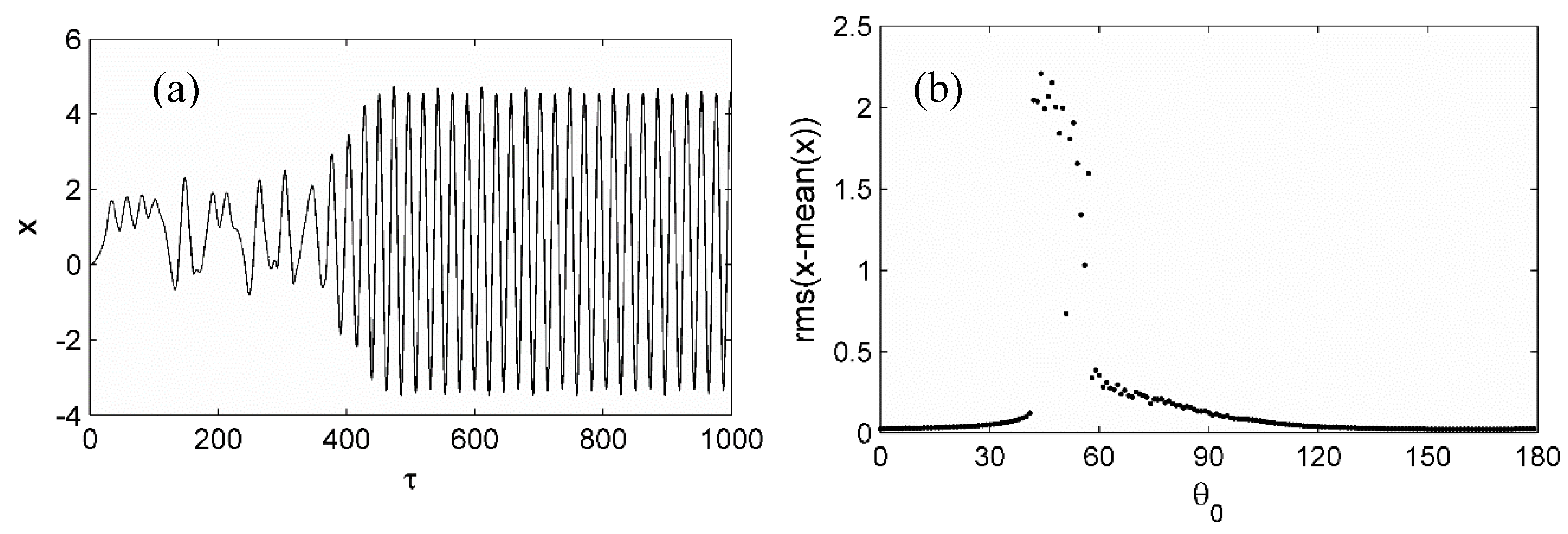
The above results indicate that the term "sprag" can be replaced by the catastrophic characteristics with changes in system parameters such as the initial inclined angle ${\theta }_o$. In the sliding oscillation, the discontinuous jump can still dominates the oscillatory behavior. Figure 7a illustrates that the oscillation started from the zero initial position, $x=0$ and $y=0$ for the angle ${\theta }_o=49°$, and reached the stable limit cycle. As the angle varied, the amplitude of oscillation drastically increased near the value of catastrophe, as shown in Figure 7b. It implies that the "sprag-slip oscillation" was initiated from the catastrophic behavior rather than the infinite spragging force. In this scenario, the sliding equilibrium met the catastrophe, lost the balance of forces, and then sought the adjacent attractor. It required large sliding deformation, leading to the limit cycle oscillation. This will be called "catastrophe-type oscillation" in frictional sliding system.

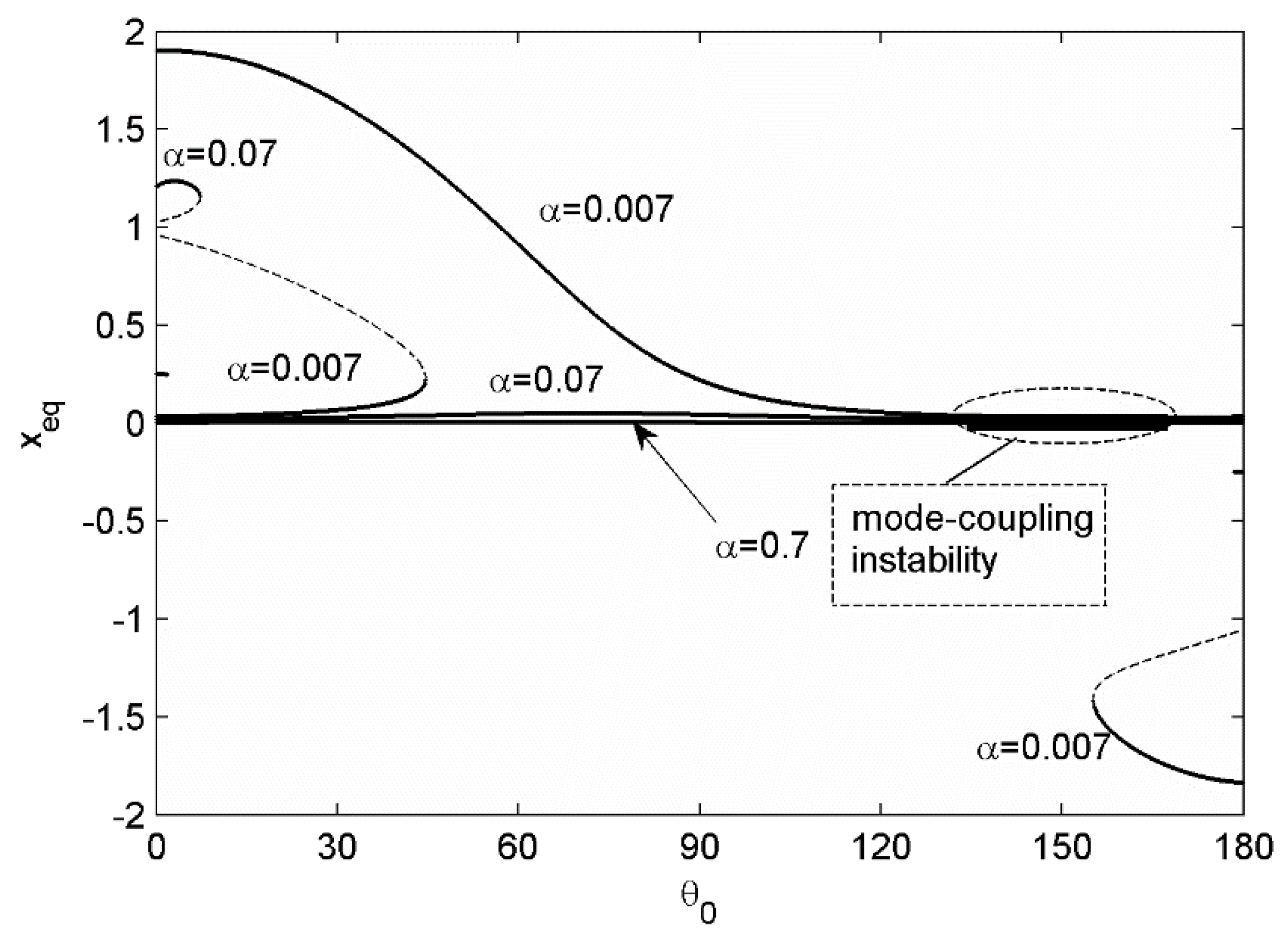
The influence of system parameters on the catastrophe was numerically investigated. The steady-sliding equilibrium curves were calculated with the three different values of system parameters with respect to ${\theta }_o$. In Figure 8, the equilibrium curves are plotted with respect to $\beta =0$, 1, and 2. If the steady-sliding equilibrium in the sliding direction started near the zero sliding deformation, the catastrophe took place for $\beta =0$ and 1. However, its trajectory with $\beta =2$ did not cross the catastrophe, but became a smooth curve. Similarly, for the steady-sliding equilibrium starting near the zero sliding deformation in Figure 9, the catastrophe occurred only for $\alpha =0.007$, whereas the others for $\alpha =0.07$ and $\alpha =0.7$ toke smooth curves as well. In this example, the flutter instability due to mode-coupling took place for $\alpha =0.7$ around ${\theta }_o={150}^{°}$. It should be noted that the stable steady-sliding was changed dynamically unstable if the condition of mode-coupling instability was met [17]. Figure 10 illustrates the effect of $\sigma$ where the steady-sliding starting near the zero sliding deformation met the catastrophe for $\sigma =0.1$ and 1, but not for $\sigma =0.01$. It is also seen that one of the stable equilibriums for $\sigma =1$ can become dynamically unstable due to mode-coupling mechanism.

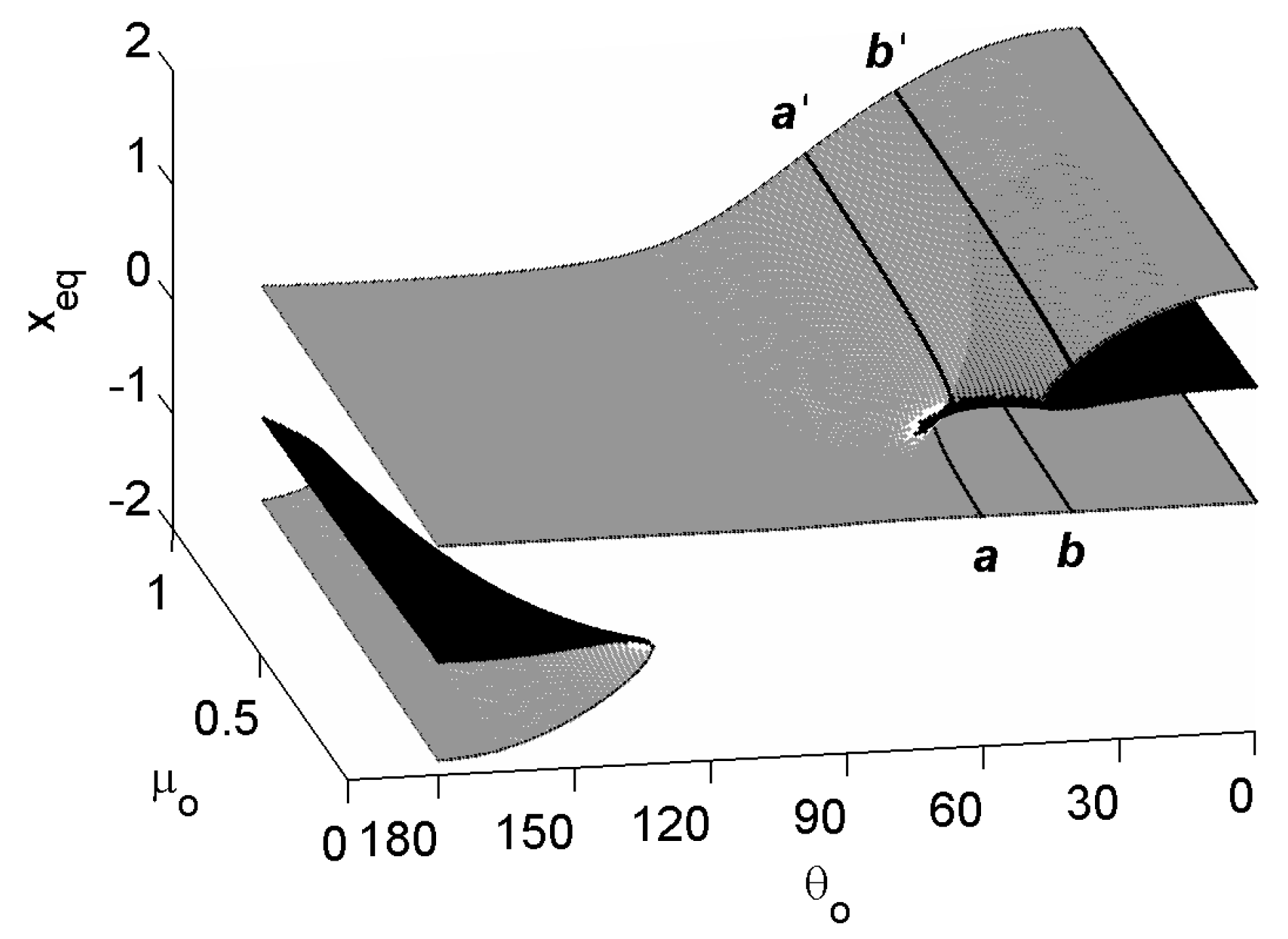
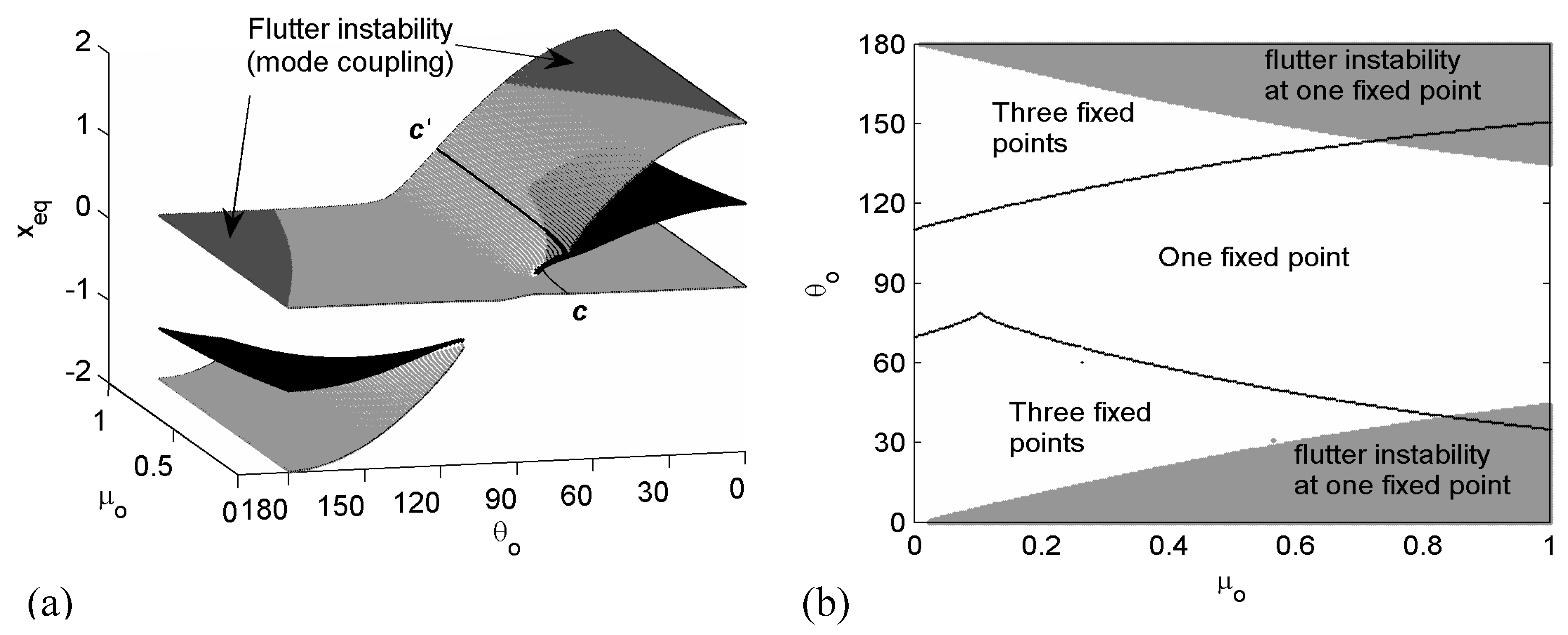
In order to illustrate the possibility of the catastrophe-type oscillation in relation to the friction coefficient, the solution surface of the fixed points was plotted in the topological sense with two control variables, ${\theta }_o$ and ${\mu }_o$, as shown in Figure 11. Such surface allowed us to investigate the dynamic behavior in a nonlinear compliant system with friction. For given values, one or three steady-sliding equilibriums were possible where one central surface was divergent and the upper and lower surfaces were stable. There must be the bifurcation set, which separates the single solution set from the triple one. To demonstrate this, the bifurcation set was plotted in the figure of control variables, as shown in Figure 12. At the bifurcation set, the state of system must jump to another state. Such jump can take place twice for a given ${\theta }_o$ if the state is on the cusp of bifurcation curve, which is the cusp catastrophe. In the cusp catastrophic behavior, the trajectory (a-a’ in Figure 11) took hysteresis where the reverse path was not same as the original one, as illustrated in Figure 13a. On the other hand, Figure 13b shows that the trajectory in the single jump condition (b-b’ in Figure 11) did not return to the original. Figure 14 indicates that the surface of the stable steady-sliding equilibrium set can also be separated with the set of dynamically unstable equilibriums by the Hopf bifurcation for the specific system parameters.

4. Discussions

We developed the nonlinear sliding system with the variable angle of the inclined spring in order to examine the sprag-slip oscillation. Nonlinear equilibrium equation was calculated by converting into the form of the polynomial equation. From the equilibrium solution, the infinite spragging force was found only for the constant angle of the inclined spring, which is the linear sprag model. However, the spragging force is always bounded if the angle of the inclined spring is set to be variable. Also, it was found that the catastrophic static deformation in the steady-sliding state can occur. Consequently, the catastrophe in equilibrium curve can lead to the large oscillations. Therefore, it was concluded that the ’sprag’, termed by Spurr [1], can be described by the catastrophic characteristics of the frictional sliding system in association with the angle of the inclined spring.

We also illustrated that the cusp catastrophe can take place for certain system parameters depending on the inclined angle of spring and the friction coefficient. The bifurcation set was demonstrated on the topological surface of the steady-sliding equilibrium over the parametric space,${\mu }_o$ and ${\theta }_o$. In some cases, the flutter instability due to mode-coupling mechanism was found on the equilibrium surface.

This catastrophic behavior in the friction-sliding system was proposed using a simple but highly nonlinear spring-mass system. It implied that a real mechanical system with a highly nonlinear geometry such as an inclined and hinged spring can have multiple equilibria. When the number of equilibria changes with respect to system parameters, this type of catastrophic sprag-slip oscillation can occur in the real system.

For a friction-sliding system with kinematically variable stiffness, sprag-slip is the one potential mechanism producing unwanted vibrations. In order to predict the sprag-type oscillation, therefore, the kinematic variation of system stiffness should be precisely estimated during sliding. If so, the sprag-slip oscillations can be predicted in numerical real-time simulation.

In future work, we will demonstrate and validate the sprag-slip oscillation through experiment using the system configuration that was suggested in this analytical model.