Abstract
Conventional data augmentation (DA) techniques, which have been used to improve the performance of predictive models with a lack of balanced training data sets, entail an effort to define the proper repeating operation (e.g., rotation and mirroring) according to the target class distribution. Although DA using generative adversarial network (GAN) has the potential to overcome the disadvantages of conventional DA, there are not enough cases where this technique has been applied to medical images, and in particular, not enough cases where quantitative evaluation was used to determine whether the generated images had enough realism and diversity to be used for DA. In this study, we synthesized 18F-Florbetaben (FBB) images using CGAN. The generated images were evaluated using various measures, and we presented the state of the images and the similarity value of quantitative measurement that can be expected to successfully augment data from generated images for DA. The method includes (1) conditional WGAN-GP to learn the axial image distribution extracted from pre-processed 3D FBB images, (2) pre-trained DenseNet121 and model-agnostic metrics for visual and quantitative measurements of generated image distribution, and (3) a machine learning model for observing improvement in generalization performance by generated dataset. The Visual Turing test showed similarity in the descriptions of typical patterns of amyloid deposition for each of the generated images. However, differences in similarity and classification performance per axial level were observed, which did not agree with the visual evaluation. Experimental results demonstrated that quantitative measurements were able to detect the similarity between two distributions and observe mode collapse better than the Visual Turing test and t-SNE.
1. Introduction
Approximately 50 million people worldwide have dementia, and nearly 10 million new cases occur each year. This number is expected to increase to 82 million by 2030 and 152 million by 2050 [1,2]. Alzheimer’s disease (AD), which is present in 70% of patients with dementia, is the most prevalent dementia-causing illness. It degrades memory and, thinking skills and eventually renders a person unable to maintain an independent life [3]. From a neuropathological point of view, the main factor responsible for the symptoms of AD are intracellular neurofibrillary tangles and extracellular amyloid plaques [4,5,6,7]. Positron emission tomography (PET) is an ultrasensitive and non-invasive molecular imaging technique used to detect functional activity within organs that are expected to be disease-related by observing the spatiotemporal distribution of radiotracers [8]. Currently, tau-PET, which observes neurofibrillary tangles, is only used for research purposes [9], but amyloid-PET, which has been approved by the Food and Drug Administration, is used as a clinically important indicator in the diagnosis of dementia [10]. In particular, as specific changes in beta amyloid (Aβ) deposition within the brain are reported to occur earlier than changes in glucose metabolism, gross cortical atrophy, or other biomarkers, PET and related techniques are expected to provide important biomarkers that can be used for early diagnosis and prediction of AD [4,5].
In analytical research for medical imaging, statistical analysis and machine learning (ML) represent informative analytical techniques that have provided new understanding and insight into the pathological characteristics of disease [11,12]. In particular, deep learning (DL) technology, which is a type of ML, has recently successfully been applied to various medical imaging techniques, and has demonstrated its potential to address diverse problems such as classification [13,14], segmentation [15,16], detection [17,18,19], and reconstruction [20,21,22]. Most DL-based models achieve high abstraction or predict posterior probabilities for a certain class by finding the proper combination of non-linear operations. In this process, the deeply stacked model parameters connecting the input to the output (deep neural network) are fitted to “appropriate training set” to create a function that is general enough to make predictions. Therefore, in DL technology, the generalization performance encourages the practitioner to obtain (1) sufficient numbers, (2) balanced numbers for each class distribution, and (3) correctly labeled training sets for supervised learning problems [13,18]. However, in most research environments, including medicine, it is difficult to obtain large number of relevant and highly qualified dataset that can provide these rich experiences. As a result, the DL research community has also conducted a variety of studies in which a given problem with constraints was solved using a small number of training datasets or datasets with incomplete or roughly drawn labels [16,23,24].
Augmenting a given training data, which is known as data augmentation (DA), is frequently used across domains to improve the generalization capabilities of DL models. DA techniques have been utilized in various DL-based image classification tasks because they are intuitive and easy to implement [25,26]. The conventional DA for image data repeatedly applies a pre-defined operation (e.g., translation, rotation, or mirroring) to the input images in a training set, which allows the target model to be trained to learn additional features that are robust to changes in the operation. If the image generated as a result of such a DA operation is sufficiently homogeneous with the training data, it could also be expected to prevent overfitting caused by a relatively heavy DL-based model compared to the size of the insufficient training set [24]. However, there are some limitations to consider before applying the existing conventional DA techniques to medical images. First, the experimenter must decide which transformations to apply to the original data so that the data generated by the transformation is similar with that of the real distribution. In other words, the distribution of the transformed dataset must maintain homogeneity for the class to which it belongs, and heterogeneity for other classes to which it does not belong. Second, changes in conventional DA in multi-dimensional data such as images do not sufficiently simulate the distributions of various lesions. It is difficult to simulate new patterns of lesions just by applying the iterative operations of conventional DA to given medical images. For example, when the lesion is diffuse, such as in the deposition of Aβ, it is difficult to define various types of the lesion using iterative operations.
In the same vein, another interesting DA is based on the generative adversarial network (GAN), which synthesizes data to be used as training data through a generative model that learns the data distribution instead of defining operations in advance [27,28]. The GAN utilizes two modules, discriminator and generator, that compete with each other to learn fake distributions that mimic the real distribution [29]. Ideally, if the GAN can generate a real distribution, the generated distribution could show the boundaries between heterogeneous groups and have the potential to improve generalization of the target model by identifying similar patterns that are not in the training set [27]. However, previous studies on GAN-based DA have rarely considered evaluating and selecting samples quantitatively, and in some cases, performance has deteriorated or been minimal after GAN-based DA [24,28].
Therefore, to successfully drive a stable GAN-based DA, determining whether to enhance the training set using the generated set based on quantitative evaluation could help to preserve and reliably improve the performance of the target model. However, no GAN-synthesized brain images have been evaluated using recently reported quantitative measurements [30] instead of traditional approaches [29,31], although some simple results of visual evaluations have been reported [32]. Furthermore, according to our investigation, studies on a GAN-based synthetic medical imaging were not addressed with a quantitative evaluation as well as a visual assessment of a brain PET for diagnosis and prognosis of dementia. In this study, we created a conditional GAN to improve the Aβ estimation model and performed a quantitative evaluation to confirm the similarity that can be expected to improve the generalization performance. This method includes (1) conditional WGAN-GP to learn each axial image distribution extracted from pre-processed 3D FBB images, (2) pre-trained DenseNet121 and model-agnostic metrics to visually and quantitatively measure the generated images, and (3) ML models such as support vector machine (SVM) and neural network (NN) for observing generalization performance after using of generated images for DA. Finally, we will upload the weights of GAN models, and the source code for our experiments (https://github.com/kang2000h/GAN_evaluation) so that the experiments we performed have reproducibility and persistence for related works (Supplementary Materials).
2. Materials and Methods
2.1. Experiment
A data flow diagram is shown in Figure 1 that illustrates the process of obtaining GAN to improve the target model using augmented FBB amyloid brain PET image data and measuring the reality of the generated data and its suitability for use in data augmentation. First, raw PET images obtained from a PACS running at DAUH undergo pre-processing. The pre-processed images were examined, and 3D images from patients that were Aβ negative or Aβ positive were divided using a 1:1 ratio into training and test sets. The training set was used to select and train GAN models that generated images of both groups. In this experiment, the similarity between the images generated from the trained GAN model and the real images was evaluated using a Visual Turing test, distribution with t-SNE, and 3 quantitative metrics. The metrics selected to measure a similarity of a given data distribution in this experiment used recently reported model-agnostic metrics [30,33] including Maximum mean discrepancy (MMD), Fréchet inception distance (FID), and The 1-nearest neighbor classifier (1-NN) leave-one-out (LOO) accuracy instead of traditional approaches in which the their limits are reported [34]. Finally, the generalization performance of the target model was measured by comparing the performance of a target model that was trained using only the training set with the augmented target model that was trained using both the training and generated sets.
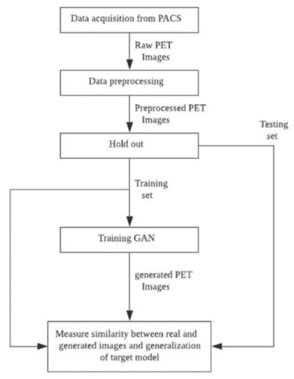
Figure 1.
Data flow diagram summarizing the experimental process.
The tool used in this experiment was written using Python 3.6.9 (Python Software Foundation, Wilmington, DE, USA), and Keras 2.2.4, and OpenCV 4.1.2.30 libraries were mainly used. DenseNet was used as a feature extractor, and finetuned weights were provided by the Keras library. The experimental environment ran on Linux Ubuntu 16.04 LTS with 4 NVIDIA GeForce GTX TITAN XP GPU.
2.2. Data Acquisition and Pre-Processing
The FBB PET/CT images used in this study were collected retrospectively from images taken at the Department of Nuclear Medicine, Dong-A University Hospital (DAUH) from November 2015 to May 2018. The Institutional Review Board of Dong-A University Hospital reviewed and approved this study protocol (DAUHIRB-17-108). Each FBB image was confirmed by a nuclear medicine physician after collection to ensure that the Aβ distribution labels were accurate. The labeling work performed for our experimental data was based on the brain amyloid plaque load (BAPL) scoring system for reading existing FBB images. Four areas of the brain including the frontal lobe, temporal lobe, parietal lobe, and posterior cingulate were observed in the axial plane and scored based on the amount of Aβ deposited on the gray matter against the white matter [35,36]. All subjects photographed in this study received clinical diagnosis by DAUH, a neurologist. There were 298 participants in the data group, which included 160 typical Aβ negatives and 138 typical Aβ positives. Detailed demographic data are presented in Table 1. The FBB PET images used in this experiment were taken using a Biograph 40mCT Flow PET/CT scanner (Siemens Healthcare, Knoxville, TN, USA) and reconstructed via UltraHD-PET (TrueX-TOF). The participants were photographed 90 min after an FBB (NeuraCeq, Piramal, Mumbai, India) dose of 300 mBq was intravenously injected and images were taken 20 min after Helical CT with a 0.5 s rotation time at 100 kVp and 228 mAs. The raw PET images used in this experiment were resliced from a field of view of 408 × 408 × 168 (mm) and stored in the DICOM format in the DAUH PACS.

Table 1.
Demographics of subjects who were photographed with FBB images retrospectively collected at Dong-A University Hospital.
The pre-processing steps, including co-registration and spatial and count normalization for the brain images applied in this experiment, were performed based on statistical parametric mapping 8 [37]. Rigid co-registration was first performed on each PET image and the corresponding CT image with respect to the center. An in-house PET template was created using CT images from 21 patients without typical AD and 9 patients with typical AD along the MNI space. Spatial normalization was performed on each PET image using the generated PET template [38,39,40]. Then, stochastic cerebellar masks for the PET templates were obtained from PMOD3.6 (PMOD Technologies Ltd., Zurich, Switzerland) and the Hammers brain atlas [41], and these were used to perform count normalization based on cerebellar intensity [42]. After pre-processing, the input data for the Aβ classifier was extracted and only the 15–50 th axial images so that only the axial plane that was read by the nuclear medicine physician was examined. Finally, a 95 × 79 × 36 image representing the Aβ distribution of each subject was used as an input for the GAN and target classifier models.
2.3. Target Model to Enhance with Generated Set
Before elucidating the design of a generative model in Section 2.4, we first defined the target model for which the images created from the generative model in this experiment will be trained. Previous studies [43,44] have shown that the performance of the ML/DL-based classification system for the Aβ distribution on FBB amyloid PET image data obtained from DAUH was 92.38% and 93.37%, respectively. Brain images generated using various modalities such as Magnetic Resonance Imaging (MRI), CT, and PET maintain spatial, and, depending on the conditions, temporal information of more than 3-dimensions. Therefore, various designs can be adopted depending on the features and pathological characteristics of the target lesion [45]. When evaluating PET images for the presence of FBB amyloid, the nuclear medicine physician makes a reading decision based on the contrast of gray matter observed through the axial plane of the FBB Aβ PET. Therefore, in a previous study [43,44,46], the BAPL score of a given FBB PET was estimated based on the Aβ distributions found at each axial level, also known as regional cortical tracer uptake (RCTU), instead of extracting the features from the 3D information according to the current process used by physicians.
In this experiment, we used the main method described in previous studies as target classifier to observe the effectiveness of GAN-based DA with visual and quantitative similarity. Therefore, the object classifier used in this experiment consists of a feature extractor to reduce features from the 2D axial plane and a classifier to predict the Aβ distribution from the extracted features. We used DenseNet [47], a well-known convolutional neural network (CNN) structure, as the feature extractor, and the support vector machine (SVM) [48] and neural network (NN) as the classifiers. Figure 2 shows the simplified structure of the target model used in our experiment. Transfer learning is a technique that applies a model that has learned data in a specific field to similar or completely different fields, and is used in medical image classification using DL-based classifiers to report interesting results [13,14]. It is a way to reuse the weights of a finetuned CNN model that are mostly trained with ImageNet datasets [49]. In particular, In a case that an input medical image is a originally gray scale (e.g., ultrasonography, MRI, and PET), previous studies which use the conversion of gray to RGB reports feasible performance even with an unknown artifacts and increased complexity [50,51]. Although the input of the target model was FBB PET images which is originally a gray scale version of a real PET image, the channels of the input data were transformed into a color channel using the OpenCV-python library to match the channel size of the finetuned DenseNet model for a continuity and reproducibility of previous studies [43,44,46]. Target model training and model selection validation were performed using 4-fold nested cross-validation and Bayesian optimization for SVM. The search space for hyper-parameters for SVM was set to kernel functions in (Linear, RBF, Poly), C in [1, 100], gamma in [0.0001, 0.1], and for NN was deterministically set to 3 hidden layers with 128,128, and 64 nodes, respectively; Adam optimizer with β1 = 0.9, β2 = 0.999, and without decay; 300 epochs; and learning rate 0.00005.
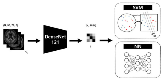
Figure 2.
Target model scheme to measure the generalization performance after data augmentation based on the generative adversarial network.
2.4. Generative Adversarial Network for Data Augmentation
The target classifier we chose performs inferences on the 2D axial images, while the prediction for the Aβ distribution for a subject should reflect the 36 axial planes placed on the transverse axis. Therefore, to assist the target classifier, the GAN model must understand all of the Aβ deposition patterns for the 36 axial plane levels, with the anatomical information matched to each level. Thus, we followed the structure of the discriminator and generator of the Deep Convolutional Generative Adversarial Network (DCGAN) [52] to learn and infer the Aβ deposition patterns on a axial plane level, and trained each of the axial levels from 0 to 35 to which the input image belongs using additional condition labels [53]. Repeatedly stacked blocks were used to construct a network structure for both generator and discriminator, and the inputs for each module multiplied by the encoded vector for each axial level label stored in an embedding matrix and then entered the stacked network. A generator produced an image from a noise vector of size 300 sampled from a normal distribution, and a discriminator estimated a score for the similarity of the two distributions from real and generated images as a critic. The generator consisted of first hidden layer with 8192 nodes connected to the noise vector, and 5 layers of blocks which had up-sampling, convolution, batch normalization, and activation function. The activation function of the last block was tanh instead of ReLU which other blocks had. The discriminator had 4 layers of blocks which had convolution, batch normalization, leaky ReLU (α = 0.2), and dropout layer (p = 0.25). And a global average pooling and a dense layer followed the blocks ahead. The structure of the GAN model used in this experiment is shown in Figure 3.
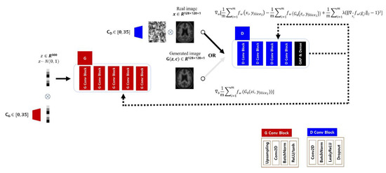
Figure 3.
Structure of generative adversarial network to enhance data for a specific disease. The amyloid negative or positive dataset were used for training independent generator (G) and discriminator (D) with a condition indicating an axial level label (CG and CD).
The GAN learns a function that connects the target distribution directly from the input distribution without any estimation of the probability density function for the target domain. GAN has a mechanism in which the two models, Generator G and Discriminator D, learn from each other competitively [29] via Equation (1):
Discriminator D predicts the probability that the received data belongs to the real distribution . To maximize V(D, G), D should ideally predict 0 for the generated data G(z) from Generator G, which learns the parameters such that D(G(z)) = 1 to minimize V(D, G).
In our experiments implementing Wasserstein GAN (WGAN) and the loss, the input image X of the discriminator parameterized by w, called critic in the original paper [54], and the input vector Z of Generator parameterized by , are in the real spaces and , respectively. Since the image synthesized by Generator follows the distribution , and is also the same as , then
Let the given PET image samples be {}, which is i.i.d, and the training set for the GAN and target model is the axial plane {} extracted from and are on . has two labels, an Aβ class [0, 1] and an axial label class [0, 35], respectively. We aimed to obtain a generative model that produces that is sufficiently close to .
In the previously reported WGAN [54], a weight clipping method was used to simply implement a Discriminator following the 1-Lipschitz constraint with a gradient between two points less than 1. Gradient penalty (GP) loss [55] was proposed to reduce the length of time needed to reach an optimality when the weights are too large or too small. We challenged the model to satisfy the constraints by adding a regularization term (Equation (10)) to the Wasserstein loss (Equation (9)) so that the gradient norm is 1 through the weighted average between the points sampled from and via Equation (6):
Model optimization was performed by joint loss (Equation (7)) for both and , and each of the parameters and were optimized by RMSProp [56], respectively, via Equations (10) and (11):
To augment Aβ negative and positive images for each class, the GAN model was constructed as two independent models, and the generated images were used as training data for the target model to improve the generalization.
2.5. Performance Metrics
Visual and quantitative metrics were used to evaluate the degree of similarity between the images generated by the generator and the test set. The generated images were visually evaluated by comparing them with real images in test set using the Visual Turing test [32] and observing the distribution of image features using the t-SNE [57]. In the quantitative evaluation, features were extracted from the image, and the similarity between the extracted feature distributions was measured using 3 model-agnostic metrics. All feature extraction processes were performed using the finetuned DenseNet121 model. Because each image contained many slices, representative images were selected at equal intervals from all 36 images at low levels (beginning in the region where the cerebellum was observed). We selected 6 representative axial planes to cover the four brain regions required by the BAPL scoring system.
2.5.1. Visual Turing Test and Feature Visualization
In the Visual Turing test, 2 parameters, a specific Aβ group (negative or positive) and a slice of the level to be evaluated, were determined, and then 40 samples were randomly extracted for each of the real and generated images. Using a GUI program written in the Python tkinter library, the randomly extracted real and generated images were presented at the same time to the evaluator who was asked to select the images that they thought were real. The GUI program was developed and tested on Windows 10 and installed in the Department of Nuclear Medicine, DAUH to allow physicians and researchers to participate in the Visual Turing Test. The results of the test were an accuracy estimated from the number of real images the evaluator found exactly.
Feature visualization begins by extracting features from the real and generated images for each class label. The extracted feature by DenseNet121 model were 1024-D, and reduced in 2-D using t-SNE (perplexity = 40.0). This feature extraction was followed by centering the mean to zero and scaling to unit variance. This process was performed for the Aβ groups and at each axial view level for the training, test, and generated set to observe the distribution.
2.5.2. Quantitative Measure
We used model-agnostic metrics reviewed in Xu et al. [30] to quantitatively measure the similarity of the distribution between real and generated images in our experiments. The 3 metrics ρ used in this experiment measure the similarity between and . It has been reported that the feature space is more advantageous for measuring the similarity of the distribution than the pixel space, and the selection of features to be extracted is also crucial [30]. Thus, for an arbitrary feature extractor Φ(.), the metric can be described as follows:
MMD measures how different and are for a given empirical kernel function k. The higher the measured value, the more the two inputs are interpreted as being different [58]. We used Gaussian functions as kernel functions,
FID is the Fréchet distance (d) between the Gaussian distribution with mean obtained from and the Gaussian distribution with mean obtained from [59,60]. FID uses features extracted from a trained network structure, such as an inception network, to measure the similarity between the distributions. The FID is defined as
The 1-NN classifier proposed by [61] as a binary classifier for two sample test statistics sets the label of the real image to 0 and the label of the generated image to 1, and can measure the similarity of the generated images by estimating the LOO accuracy. The closer the LOO accuracy is to 50%, the closer is to . As shown in [30], the LOO accuracy of 1-NN can be used to detect the tendency of mode collapse, which is difficult to detect with the human eye without special training and careful model selection. It can also robustly measure the similarity between distributions with small transformations in the feature space.
2.6. Statistical Analysis
The data collected in this experiment were statistically analyzed using MedCalc software version 18.9.1. First, for the experimental data collected retrospectively, we examined whether there was a bias involved in the formation of the Aβ distribution, other than for the diagnosis or result of cognitive function test that could be estimated based on Aβ deposited in the cerebrum. After applying the GAN-based DA, we statistically evaluated differences in the generalization performance of the ML-based model for each axial plane.
Discrete variables such as age, education, and K-MMSE that were used in the calculation of demographic data were first analyzed using the Kolmogorov-Smirnov normality test before applying the Mann-Whitney U test or t-test was applied to determine if there were differences between the distributions of Aβ groups. For continuous variables such as generalization performance, the difference in the distribution of the accuracy measured per axial level before and after GAN-based DA was analyzed using the same statistical tests that were used to evaluate discrete variables. Categorical variables, such as diagnostic results, were examined using the Chi-squared test. The statistical significance level α was 0.01, and a two-sided test was performed.
3. Results
First, we statistically confirmed that there was no bias in the other variables except for the distribution of each patient’s disease and its dependent variables (K-MMES) in the experimental dataset used in this study. Then, we used quantitative measurements to examine the generalization performance of ML models. Figure 4 shows the real pre-processed images and the GAN-based generated images that were randomly extracted without cherry picking. Section 3.2 and Section 3.3 provide a detailed explanation of the results for the representative axial planes showing the temporal lobe (TL), frontal lobe (FL), posterior cingulate and precuneus (PP1 and PP2), and parietal lobe (PL1 and PL2), instead of the total results for all 36 slices.
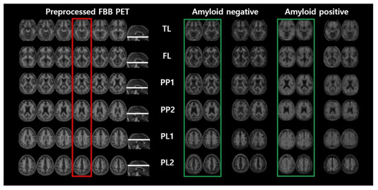
Figure 4.
Pre-processed FBB PET image and randomly picked real and generated images by the generator selected from our experiment.
3.1. Demographic Data
As shown in Table 1, the demographic data summarizes the p-values that represent statistically significant differences in age, sex, education, K-MMSE, and diagnosis. The Mann-Whitney test was performed on age, education, and K-MMSE data because the Kolmogorov-Smirnov test showed no normality ( < 0.0001, = 0.0916, = 0.0802). The chi-squared test showed no significant difference in the sex ratio between the two groups ( = 0.105), and only the distribution of diagnosis was significantly different between the two groups ( < 0.0001). Therefore, it can be assumed that the FBB image data sets used in the experiments were collected without any bias in age, gender, or years of education, except for the actual disease diagnosis and cognitive function.
3.2. Visual Turing Test
We performed the Visual Turing test [32] on real and generated images to evaluate how similar the FBB images that were generated by the GAN were to real images, and the results are shown in Figure 5. The proportions matched at the FL, PP2, and PL2 levels in the Aβ-negative group, and the FL and PP2 levels in the positive group did not exceed 50%. The axial level that visually demonstrated the greatest similarity in the Aβ-negative group was the TL level (60%), and it was the PP1 level (67%) in the Aβ-positive group. Although there was a difference in relative similarities among representative axial planes, all of them were shown to be similar with the real images.
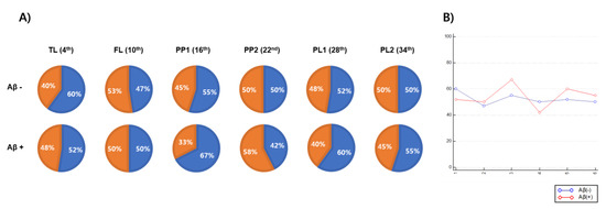
Figure 5.
The results of Visual Turing test used to validate the similarity between real and generated FBB amyloid images. (A) Each pie chart represents the proportion of real images which an experimenter find correctly (blue) with the proportion of real images which the experiment when the real and generated images are simultaneously output to the experimenter per a representative axial level including temporal lobe (TL), frontal lobe (FL), posterior cingulate/precuneus 1 (PP1), posterior cingulate/precuneus 2 (PP2), parietal lobe 1 (PL1) and parietal lobe 2 (PL2). (B) A graph showing the accuracy (y-axis) with which an experimenter correctly distinguishes real images from real and generated images according to representative axial level (x-axis).
3.3. Feature Visualization
To observe the overall distribution between real and generated images in each Aβ-negative and positive image, we acquired the image features extracted using the DenseNet121 model from the input image observed at any axial plane level. The t-SNE technique was used to observe a two-dimensionally reduced distribution. Figure 6 shows scatter plots that visualize the features reduced by t-SNE. The distribution of training and test images in the Aβ-negative group almost overlapped in all representative axial planes. However, although the FBB images used in the experiments were representative typical Aβ-negative and positive cases, the Aβ-positive images in the training or test datasets rarely appeared in the distribution of negative groups (FL, PP1, PP2, and PL2). In addition, the real images from the Aβ-negative group were not included in the Aβ-positive distribution. The distribution of GAN-generated images used to augment the training dataset primarily overlapped with the distribution of real images at the PP1 and PP2 levels for both the Aβ-negative and positive datasets, and no sample invading other class distributions was seen.
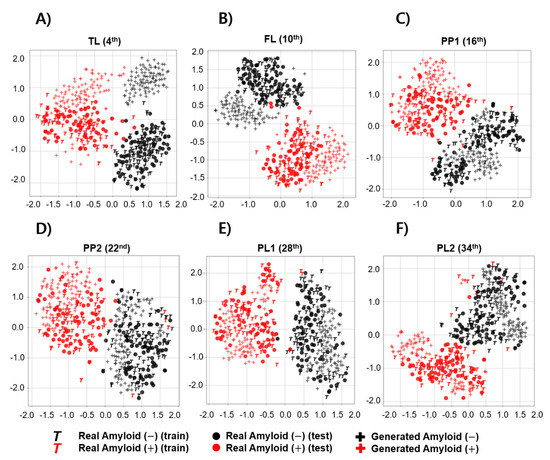
Figure 6.
Feature visualization comparing the distribution between real and generated images according to brain amyloid distribution using t-SNE. Each scatter plot represents feature visualization according to a representative axial level including (A) temporal lobe (TL), (B) frontal lobe (FL), (C) posterior cingulate/precuneus 1 (PP1), (D) posterior cingulate/precuneus 2 (PP2), (E) parietal lobe 1 (PL1) and (F) parietal lobe 2 (PL2).
3.4. Quantitative Measurements
Figure 7 shows the similarity between the real and generated set , Φ()) and between the training and test set , Φ()) measured over the entire axial level. Instead of changing the scale to [0, 1], the values on the graphs in Figure 7 are the values directly calculated from a metric. , Φ()) and , Φ()) were compared for both the Aβ and axial level classes. Contrary to the results of visual evaluation, the similarity of GAN-based synthetic images differed over axial level classes regardless of the metric used, and generally the lower and higher the axial level, the lower the similarity. Ideally, the similarity between real distributions should not vary with Aβ or axial level class, but diverse variance existed according to the metrics used. In MMD and FID, the change within each range for , Φ()) was greater than that of , Φ()). Meanwhile, when the 1-NN LOO accuracy was evaluated, the difference in the ranges of , Φ()) and , Φ()) appeared relatively small. The MMD and 1-NN LOO accuracies were the apparent similarities between , Φ()) and , Φ()) at the axial level; however, similar FID measurements were obtained at or near the 22-th axial level.
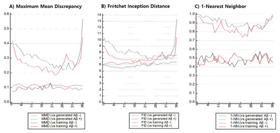
Figure 7.
Quantitative measurements to estimate synthetic similarity between real and generated images with respect to each axial level of pre-processed FBB imaging.
Table 2 compares the similarity values between , Φ()) and , Φ()) measured in the representative axial plane using MMD, FID, and 1-NN LOO. When evaluating Aβ-negative images according to quantitative metrics, the representative axial levels that appeared the most similar to real images were PL1 (MMD: 0.2284), PP2 (FID: 6.8253), and PP1 (1-NN LOO accuracy: 0.8562), and each of the metrics identified different levels as the most similar. A set of generated Aβ-positive images, meanwhile, were similar to real images in PP2, regardless of the selection of quantitative metrics (MMD: 0.1865, FID: 5.8919, 1-NN LOO accuracy: 0.7391). For all 3 metrics, the GAN model used in the experiment produced more realistic synthetic images for Aβ-positive images than the Aβ-negative images.
Table 2.
Comparison of synthetic similarity using quantitative measurements of amyloid negative and positive images.
3.5. Generalization Test
To statistically evaluate the differences in generalization performance for each axial level before and after GAN-based DA, we built one model (non-augmented) that was trained using only the training set and another model (augmented) that was trained using both the training and generated sets. The model was evaluated independently for each axial level class using the same test set. The Mann-Whitney U test was used because the given distribution was not found to exhibit normality.
Figure 8 shows a comparison of the generalization performance of the target model based on ML with and without the data generated in the training set. Regardless of the augmentation, the classification performance of the target model tended to decrease at both ends. In both models, SVM and NN, GAN-based DA was performed independently at each axial level, resulting in a statistically significant improvement in generalization performance. Thus, DA was confirmed to work with stronger evidence in the NN-based model rather than the SVM-based model (median-SVM: 0.943 to 0.956, p < 0.0454; median-NN: 0.946 to 0.963, p < 0.0047).
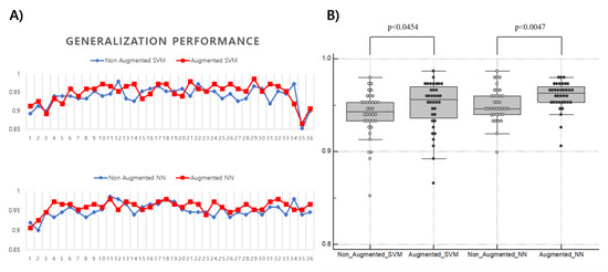
Figure 8.
Comparison of the generalization performance of ML-based classifiers before and after GAN-based data augmentation. (A) Changes of generalization performance (y-axis) of support vector machine and neural network observed at each axial level (x-axis); (B) Difference in generalization performance (y-axis) of ML models before and after GAN-based data augmentation (x-axis). Each ML model for the axial level generally improved with statistical evidence after data augmentation.
4. Discussion
4.1. Medical Image Synthesis with Quantitative Measurements
In a previous study [62] dealing with the synthesis of brain-structured MRI, a GAN structure that appropriately augments the input image domain is proposed, and some related studies comparing the performance of each generalization when the training steps of various classifiers were enhanced using generated images have been reported [27,28,32,63,64,65]. These previous studies on GAN-based DA in the medical imaging field have emphasized the design of the applied GAN and the improved generalization of the target model that was trained using the augmented dataset. However, these studies only included qualitative visual evaluation, and the reasons for quantitatively evaluating the generated images before applying the GAN include:
- The practitioner cannot predict what the samples generated from GAN will look like until they are confirmed, unlike conventional DA.
- It is not easy to visually evaluate how similar the real distribution is to the generated distribution.
- Models trained without validation of augmented data may learn data that is characteristics of diseases but falls outside of a given class with an arbitrary label.
In particular, medical images can be interpreted differently because of diverse disease distributions, then quantitative evaluation of generated medical images is important. In our study, the comparison of various classifiers was excluded, but we focused on the need for visual and quantitative evaluation of the data generated from GAN.
Evaluating the synthetic DA data is to examine how identical the generated distributions are to real distributions rather than how identical the generated samples are. The classic approach is to estimate the real distribution using Parzen window estimation to measure the average log-likelihood of the generated samples [29]. This method has the advantage of being intuitive, but a recent study has shown that the estimated log-likelihood at higher dimensional space is not realistic, and above all, this study proves that it does not give a meaningful value that correlates to the reality of the given sample [34]. Another widely known method is the inception score (IS) [31], which uses the average KL divergence between and from the class label distribution estimated from the input images by an arbitrary finetuned model (e.g., inception network) to measure the quality and diversity. This method is also intuitive and is known to be correlated with human judgment, but it has the disadvantages of not detecting overfitting for samples the predictive model entirely memorizes, mode collapse for a distribution the model does not learn, or not accounting for a model trapped into bad mode [66]. To overcome these shortcomings, some variants of the inception score with KL divergence have been reported, including modified IS [67], mode score [68], and AM Score [66]. Several approaches for defining new distances in feature space have also been reported [30], including MMD [58], FID [60], and Wasserstein distance [54].
In general, the expected effects from GAN-based DA techniques include (1) generating samples that follow the same distribution as that of the real images to ensure that there are no insufficient datasets, or (2) generating similar but realistic samples to train the model on the creative pattern. In our experiment, we demonstrated the quantitative similarity of the generated images so that we should expect to see effect (1) using the GAN that was trained with loss to minimize the Wasserstein distance between the real and generated distributions. Evaluating medical image synthesis or DA using quantitative measurements may be useful for providing a baseline for future studies, or for determining the direction of next future experiments in practical studies.
4.2. Comparison between t-SNE and Quantitative Measurements
The distribution of features extracted from t-SNE in Figure 6 shows that the Aβ-positive samples of the training set infiltrated the negative distribution at specific axial levels (PP1, PP2, and PL2). However, in the quantitative evaluation of all the axial levels of the real images, there was some variance within each metric and axial level but a consistent overall similarity (Figure 7). The quantitative metrics used in this experiment represented the similarity between the given datasets as a scalar value , Φ()), and it could be difficult to explain the similarity and distribution of a few outliers or individual samples, whereas t-SNE has the advantage of providing intuitive information about the distribution of individual samples. In internal observations, however, the Aβ-positive training set samples found in the negative distribution were typical Aβ-positive images, unlike the visualization. The similarity between the real images , Φ()), represented by the quantitative evaluation (MMD, FID, and 1-NN LOO accuracy) used in this experiment, seems to represent physicians’ visual assessment rather than t-SNE in that it is measured in the same feature space using the DenseNet121.
Comparing the real test and the generated set using the Visual Turing test (Figure 5) demonstrated that, although was quite similar to for the overall axial levels, t-SNE showed dissimilar distributions at lower and higher axial levels, and the results of the quantitative evaluation also seem to agree with the trend shown by t-SNE (Figure 7, Table 2). This suggests that t-SNE and quantitative measures can be used to determine the tendency of mode collapse of generated medical images that are difficult to find or define in visual assessment. Therefore, in the comparison between real and generated sets of medical images, the analysis using DenseNet121 trained with ImageNet and t-SNE still appears to be useful along with the quantitative evaluation method.
4.3. Comparison between Model-Agnostic Metrics
As shown in Figure 7, MMD and FID were able to distinguish the similarity between the real and generated sets , Φ()) at the middle axial level and the both end levels. In contrast, the 1-NN LOO accuracy exhibited a smaller variance in the , Φ()) for each axial level than the MMD and FID shown, and even the variance of , Φ()) for Aβ-negative images is greater than , Φ()) (Table 2). The 1-NN LOO accuracy demonstrates that the variance that occurs in the similarity estimation is larger than that of MMD and FID in identical datasets owing to the nature of the estimation of classification performance, which is sensitive to the number of data [69].
MMD and 1-NN LOO accuracy showed clear differences in , Φ()), whereas FID had some axial level at which there was no difference between , Φ()) and , Φ()) (Figure 7). This suggests that the distribution of medical image samples for which the FID measures the similarity is not suitable for measuring with the FID using the Gaussian kernel, which also suggests that proper care should be taken when measuring the similarity for medical image synthesis.
4.4. Role of Quantitative Measurements in Future Generative Data Augmentation Work
After applying GAN-based DA to the Aβ predictive model and observing statistical evidence that the GAN used in our experiment can usually improve the generalization performance at an axial level, we found some challenges that may represent directions for future work. As shown in Figure 8, the generalization performance after DA shows the results of applied DA regardless of the similarity of the generated set. Consequently, after the DA of our experiment, both increases and decreases in performance were observed when measuring the generalization performance along the axial levels. In a previous study, the performance of the target model decreased when the training data was augmented using GAN [24]. This may be caused by mode collapse, which makes the target model more confused. However, in the case of our experiment, the possibility that variance is large in the process of estimating the performance of the target classifiers cannot be excluded due to the small data set. Accordingly, we statistically verify the difference in bias of generalization performance. As a result, it seems that the performance is improved from the viewpoint of the whole slice after applying GAN-based DA. In our experiments, there might be some variance due to the small size of the small dataset.
In terms of stable DA, we need proper means to prevent or predict situations where the performance is reduced by the applied DA, which is required when the generated set is produced not by simple user-defined operations like conventional DA but by a complex function that is difficult to predict. In other words, excluding generated data that is not suitable for DA may be advantageous for stable performance improvement. Studying the quantitative evaluation of DA seems to play an important role in the detection of factors degrading the generalization performance and in assessing the suitability of the training dataset for augmentation.
5. Conclusions
In this study, we synthesized 18F-Florbetaben Aβ PET images using GAN and visually and quantitatively evaluated the real and generated images. The similarity of the images that could statistically augment Aβ images was quantitatively measured for Aβ-negative (MMD:0.2284, FID:6.8253, 1-NN LOO accuracy:0.8562) and positive images (MMD:0.01865, FID:5.8919, 1-NN LOO accuracy:0.6233). We enhanced SVM/NN-based classifier using Aβ images generated by GAN (median-SVM, 0.943–0.956, median-NN, 0.946–0.963). The experimental results demonstrated that quantitative measurements were able to detect the similarity between the two distributions and to observe mode collapse better than the Visual Turing test and t-SNE.
Supplementary Materials
The following are available online at https://github.com/kang2000h/GAN_evaluation, source code, model structure, weights, and figures used in this study and paper.
Author Contributions
Conceptualization, H.K., J.-S.P., K.C. and D.-Y.K.; methodology, H.K.; software, H.K.; validation, H.K. and D.-Y.K.; formal analysis, H.K.; investigation, H.K.; resources, D.-Y.K.; data curation, H.K.; writing—original draft preparation, H.K.; writing—review and editing, H.K., J.-S.P., K.C. and D.-Y.K.; visualization, H.K.; supervision, D.-Y.K.; project administration, D.-Y.K.; funding acquisition, K.C., and D.-Y.K. All authors have read and agreed to the published version of the manuscript.
Funding
This research was supported by the National Research Foundation (NRF) of Korea funded by the Ministry of Science, ICT & Future Planning (NRF-2018 R1A2B2008178).
Conflicts of Interest
The authors declare no conflicts of interest. The funders had no role in the design of the study; in the collection, analyses, or interpretation of data; in the writing of the manuscript, or in the decision to publish the results.
References
- World Health Organization. Dementia. Available online: https://www.who.int/news-room/fact-sheets/detail/dementia (accessed on 25 November 2019).
- World Health Organization. Risk Reduction of Cognitive Decline and Dementia: WHO Guidelines; World Health Organization: Geneva, Switzerland, 2019. [Google Scholar]
- National Institutes of Health. What Is Alzheimer’s Disease? Available online: https://www.nia.nih.gov/health/what-alzheimers-disease (accessed on 20 December 2019).
- Villemagne, V.L. Amyloid imaging: Past, present and future perspectives. Ageing Res. Rev. 2016, 30, 95–106. [Google Scholar] [CrossRef] [PubMed]
- Villemagne, V.L.; Rowe, C.C.; Macfarlane, S.; Novakovic, K.; Masters, C.L. Imaginem oblivionis: The prospects of neuroimaging for early detection of Alzheimer’s disease. J. Clin. Neurosci. 2005, 12, 221–230. [Google Scholar] [CrossRef] [PubMed]
- Michaelis, M.L.; Dobrowsky, R.T.; Li, G. Tau neurofibrillary pathology and microtubule stability. J. Mol. Neurosci. 2002, 19, 289–293. [Google Scholar] [CrossRef]
- Haass, C.; Selkoe, D.J. Soluble protein oligomers in neurodegeneration: Lessons from the Alzheimer’s amyloid β-peptide. Nat. Rev. Mol. Cell Biol. 2007, 8, 101. [Google Scholar] [CrossRef]
- Luna, A.; Vilanova, J.C.; Da Cruz, L.C.H., Jr.; Rossi, S.E. Functional Imaging in Oncology: Clinical Applications; Springer: Berlin/Heidelberg, Germany, 2014; Volume 2. [Google Scholar]
- Leuzy, A.; Chiotis, K.; Lemoine, L.; Gillberg, P.-G.; Almkvist, O.; Rodriguez-Vieitez, E.; Nordberg, A. Tau PET imaging in neurodegenerative tauopathies—Still a challenge. Mol. Psychiatry 2019, 24, 1112–1134. [Google Scholar] [CrossRef]
- Marcus, C.; Mena, E.; Subramaniam, R.M. Brain PET in the diagnosis of Alzheimer’s disease. Clin. Nucl. Med. 2014, 39, e413. [Google Scholar] [CrossRef]
- Chiaravalloti, A.; Castellano, A.E.; Ricci, M.; Barbagallo, G.; Sannino, P.; Ursini, F.; Karalis, G.; Schillaci, O. Coupled imaging with [18F] FBB and [18F] FDG in AD subjects show a selective association between amyloid burden and cortical dysfunction in the brain. Mol. Imaging Biol. 2018, 20, 659–666. [Google Scholar] [CrossRef]
- Kim, J.; Hong, J.; Park, H. Prospects of deep learning for medical imaging. Precis. Future Med. 2018, 2, 37–52. [Google Scholar] [CrossRef]
- Gulshan, V.; Peng, L.; Coram, M.; Stumpe, M.C.; Wu, D.; Narayanaswamy, A.; Venugopalan, S.; Widner, K.; Madams, T.; Cuadros, J. Development and validation of a deep learning algorithm for detection of diabetic retinopathy in retinal fundus photographs. JAMA 2016, 316, 2402–2410. [Google Scholar] [CrossRef]
- Lakhani, P.; Sundaram, B. Deep learning at chest radiography: Automated classification of pulmonary tuberculosis by using convolutional neural networks. Radiology 2017, 284, 574–582. [Google Scholar] [CrossRef] [PubMed]
- Ronneberger, O.; Fischer, P.; Brox, T. U-net: Convolutional networks for biomedical image segmentation. In Proceedings of the International Conference on Medical Image Computing and Computer-Assisted Intervention, Munich, Germany, 5–9 October 2015; pp. 234–241. [Google Scholar]
- Pathak, D.; Krahenbuhl, P.; Darrell, T. Constrained convolutional neural networks for weakly supervised segmentation. In Proceedings of the IEEE International Conference on Computer Vision, Santiago, Chile, 7–13 December 2015; pp. 1796–1804. [Google Scholar]
- Jiang, H.; Ma, H.; Qian, W.; Gao, M.; Li, Y. An automatic detection system of lung nodule based on multigroup patch-based deep learning network. IEEE J. Biomed. Health Inform. 2017, 22, 1227–1237. [Google Scholar] [CrossRef] [PubMed]
- Hwang, E.J.; Park, S.; Jin, K.-N.; Im Kim, J.; Choi, S.Y.; Lee, J.H.; Goo, J.M.; Aum, J.; Yim, J.-J.; Cohen, J.G. Development and Validation of a Deep Learning–Based Automated Detection Algorithm for Major Thoracic Diseases on Chest Radiographs. JAMA Netw. Open 2019, 2, e191095. [Google Scholar] [CrossRef] [PubMed]
- Ding, J.; Li, A.; Hu, Z.; Wang, L. Accurate pulmonary nodule detection in computed tomography images using deep convolutional neural networks. In Proceedings of the International Conference on Medical Image Computing and Computer-Assisted Intervention, Quebec City, QC, Canada, 10–14 September 2017; pp. 559–567. [Google Scholar]
- Hwang, D.; Kim, K.Y.; Kang, S.K.; Seo, S.; Paeng, J.C.; Lee, D.S.; Lee, J.S. Improving the accuracy of simultaneously reconstructed activity and attenuation maps using deep learning. J. Nucl. Med. 2018, 59, 1624–1629. [Google Scholar] [CrossRef] [PubMed]
- Kang, E.; Min, J.; Ye, J.C. A deep convolutional neural network using directional wavelets for low-dose X-ray CT reconstruction. Med. Phys. 2017, 44, e360–e375. [Google Scholar] [CrossRef] [PubMed]
- Quan, T.M.; Nguyen-Duc, T.; Jeong, W.-K. Compressed sensing MRI reconstruction using a generative adversarial network with a cyclic loss. IEEE Trans. Med. Imaging 2018, 37, 1488–1497. [Google Scholar] [CrossRef]
- Haeusser, P.; Mordvintsev, A.; Cremers, D. Learning by Association—A Versatile Semi-Supervised Training Method for Neural Networks. In Proceedings of the IEEE Conference on Computer Vision and Pattern Recognition, Honolulu, HI, USA, 21–26 July 2017; pp. 89–98. [Google Scholar]
- Perez, L.; Wang, J. The effectiveness of data augmentation in image classification using deep learning. arXiv 2017, arXiv:1712.04621. [Google Scholar]
- Krizhevsky, A.; Sutskever, I.; Hinton, G.E. Imagenet classification with deep convolutional neural networks. In Proceedings of the Advances in Neural Information Processing Systems, Nevada, NV, USA, 3–8 December 2012; pp. 1097–1105. [Google Scholar]
- Chen, H.; Zhang, Y.; Kalra, M.K.; Lin, F.; Chen, Y.; Liao, P.; Zhou, J.; Wang, G. Low-dose CT with a residual encoder-decoder convolutional neural network. IEEE Trans. Med. Imaging 2017, 36, 2524–2535. [Google Scholar] [CrossRef]
- Frid-Adar, M.; Klang, E.; Amitai, M.; Goldberger, J.; Greenspan, H. Synthetic data augmentation using GAN for improved liver lesion classification. In Proceedings of the 2018 IEEE 15th International Symposium on Biomedical Imaging (ISBI 2018), Washington, DC, USA, 4–7 April 2018; pp. 289–293. [Google Scholar]
- Haradal, S.; Hayashi, H.; Uchida, S. Biosignal Data Augmentation Based on Generative Adversarial Networks. In Proceedings of the 2018 40th Annual International Conference of the IEEE Engineering in Medicine and Biology Society (EMBC), Honolulu, HI, USA, 17–21 July 2018; pp. 368–371. [Google Scholar]
- Goodfellow, I.; Pouget-Abadie, J.; Mirza, M.; Xu, B.; Warde-Farley, D.; Ozair, S.; Courville, A.; Bengio, Y. Generative adversarial nets. In Proceedings of the Advances in neural information processing systems, Montreal, QC, Canada, 8–13 December 2014; pp. 2672–2680. [Google Scholar]
- Xu, Q.; Huang, G.; Yuan, Y.; Guo, C.; Sun, Y.; Wu, F.; Weinberger, K. An empirical study on evaluation metrics of generative adversarial networks. arXiv 2018, arXiv:1806.07755. [Google Scholar]
- Salimans, T.; Goodfellow, I.; Zaremba, W.; Cheung, V.; Radford, A.; Chen, X. Improved techniques for training gans. In Proceedings of the Advances in neural information processing systems, Barcelona, Spain, 5–10 December 2016; pp. 2234–2242. [Google Scholar]
- Chuquicusma, M.J.; Hussein, S.; Burt, J.; Bagci, U. How to fool radiologists with generative adversarial networks? A visual turing test for lung cancer diagnosis. In Proceedings of the 2018 IEEE 15th International Symposium on Biomedical Imaging (ISBI 2018), Washington, DC, USA, 4–7 April 2018; pp. 240–244. [Google Scholar]
- Borji, A. Pros and cons of gan evaluation measures. Comput. Vision Image Underst. 2019, 179, 41–65. [Google Scholar] [CrossRef]
- Theis, L.; Oord, A.v.d.; Bethge, M. A note on the evaluation of generative models. arXiv 2015, arXiv:1511.01844. [Google Scholar]
- Barthel, H.; Gertz, H.-J.; Dresel, S.; Peters, O.; Bartenstein, P.; Buerger, K.; Hiemeyer, F.; Wittemer-Rump, S.M.; Seibyl, J.; Reininger, C. Cerebral amyloid-β PET with florbetaben (18F) in patients with Alzheimer’s disease and healthy controls: A multicentre phase 2 diagnostic study. Lancet Neurol. 2011, 10, 424–435. [Google Scholar] [CrossRef]
- Lundeen, T.F.; Seibyl, J.P.; Covington, M.F.; Eshghi, N.; Kuo, P.H. Signs and artifacts in Amyloid PET. RadioGraphics 2018, 38, 2123–2133. [Google Scholar] [CrossRef] [PubMed]
- The Wellcome Centre for Human Neuroimaging. Statistical Parametric Mapping. Available online: https://www.fil.ion.ucl.ac.uk/spm/ (accessed on 11 February 2020).
- Rorden, C.; Bonilha, L.; Fridriksson, J.; Bender, B.; Karnath, H.-O. Age-specific CT and MRI templates for spatial normalization. Neuroimage 2012, 61, 957–965. [Google Scholar] [CrossRef]
- Hutton, C.; Declerck, J.; Mintun, M.A.; Pontecorvo, M.J.; Devous, M.D.; Joshi, A.D.; Initiative, A.s.D.N. Quantification of 18F-florbetapir PET: Comparison of two analysis methods. Eur. J. Nucl. Med. Mol. Imaging 2015, 42, 725–732. [Google Scholar] [CrossRef]
- Garcia, D.V.; Casteels, C.; Schwarz, A.J.; Dierckx, R.A.; Koole, M.; Doorduin, J. A standardized method for the construction of tracer specific PET and SPECT rat brain templates: Validation and implementation of a toolbox. PLoS ONE 2015, 10, e0122363. [Google Scholar] [CrossRef]
- Hammers, A.; Allom, R.; Koepp, M.J.; Free, S.L.; Myers, R.; Lemieux, L.; Mitchell, T.N.; Brooks, D.J.; Duncan, J.S. Three-dimensional maximum probability atlas of the human brain, with particular reference to the temporal lobe. Hum. Brain Mapp. 2003, 19, 224–247. [Google Scholar] [CrossRef]
- Daerr, S.; Brendel, M.; Zach, C.; Mille, E.; Schilling, D.; Zacherl, M.J.; Bürger, K.; Danek, A.; Pogarell, O.; Schildan, A. Evaluation of early-phase [18F]-florbetaben PET acquisition in clinical routine cases. NeuroImage Clin. 2017, 14, 77–86. [Google Scholar] [CrossRef]
- Kang, H.; Kim, W.-G.; Yang, G.-S.; Kim, H.-W.; Jeong, J.-E.; Yoon, H.-J.; Cho, K.; Jeong, Y.-J.; Kang, D.-Y. VGG-based BAPL score classification of 18F-Florbetaben Amyloid Brain PET. Biomed. Sci. Lett. 2018, 24, 418–425. [Google Scholar] [CrossRef]
- Cho, K.; Kim, W.-G.; Kang, H.; Yang, G.-S.; Kim, H.-W.; Jeong, J.-E.; Yoon, H.-J.; Jeong, Y.-J.; Kang, D.-Y. Classification of 18F-Florbetaben Amyloid Brain PET Image using PCA-SVM. Biomed. Sci. Lett. 2019, 25, 99–106. [Google Scholar] [CrossRef]
- Işın, A.; Direkoğlu, C.; Şah, M. Review of MRI-based brain tumor image segmentation using deep learning methods. Procedia Comput. Sci. 2016, 102, 317–324. [Google Scholar] [CrossRef]
- Sato, R.; Iwamoto, Y.; Cho, K.; Kang, D.-Y.; Chen, Y.-W. Accurate BAPL Score Classification of Brain PET Images Based on Convolutional Neural Networks with a Joint Discriminative Loss Function. Appl. Sci. 2020, 10, 965. [Google Scholar] [CrossRef]
- Huang, G.; Liu, Z.; Van Der Maaten, L.; Weinberger, K.Q. Densely connected convolutional networks. In Proceedings of the IEEE Conference on Computer Vision and Pattern Recognition, Honolulu, HI, USA, 21–26 July 2017; pp. 4700–4708. [Google Scholar]
- Vapnik, V.N. Support Vector Machine: Statistical Learning Theory; Wiley-Interscience: Hoboken, NJ, USA, 1998. [Google Scholar]
- Russakovsky, O.; Deng, J.; Su, H.; Krause, J.; Satheesh, S.; Ma, S.; Huang, Z.; Karpathy, A.; Khosla, A.; Bernstein, M. Imagenet large scale visual recognition challenge. Int. J. Comput. Vis. 2015, 115, 211–252. [Google Scholar] [CrossRef]
- Tajbakhsh, N.; Shin, J.Y.; Gurudu, S.R.; Hurst, R.T.; Kendall, C.B.; Gotway, M.B.; Liang, J. Convolutional neural networks for medical image analysis: Full training or fine tuning? IEEE Transact. Med. Imaging 2016, 35, 1299–1312. [Google Scholar] [CrossRef] [PubMed]
- Cheng, P.M.; Malhi, H.S. Transfer learning with convolutional neural networks for classification of abdominal ultrasound images. J. Digit. Imaging 2017, 30, 234–243. [Google Scholar] [CrossRef] [PubMed]
- Radford, A.; Metz, L.; Chintala, S. Unsupervised representation learning with deep convolutional generative adversarial networks. arXiv 2015, arXiv:1511.06434. [Google Scholar]
- Mirza, M.; Osindero, S. Conditional generative adversarial nets. arXiv 2014, arXiv:1411.1784. [Google Scholar]
- Arjovsky, M.; Chintala, S.; Bottou, L. Wasserstein gan. arXiv 2017, arXiv:1701.07875. [Google Scholar]
- Gulrajani, I.; Ahmed, F.; Arjovsky, M.; Dumoulin, V.; Courville, A.C. Improved training of wasserstein gans. In Proceedings of the Advances in Neural Information Processing Systems, Califonia, CA, USA, 4–9 December 2017; pp. 5767–5777. [Google Scholar]
- Graves, A. Generating sequences with recurrent neural networks. arXiv 2013, arXiv:1308.0850. [Google Scholar]
- Maaten, L.v.d.; Hinton, G. Visualizing data using t-SNE. J. Mach. Learn. Res. 2008, 9, 2579–2605. [Google Scholar]
- Gretton, A.; Borgwardt, K.M.; Rasch, M.J.; Schölkopf, B.; Smola, A. A kernel two-sample test. J. Mach. Learn. Res. 2012, 13, 723–773. [Google Scholar]
- Dowson, D.; Landau, B. The Fréchet distance between multivariate normal distributions. J. Multivar. Anal. 1982, 12, 450–455. [Google Scholar] [CrossRef]
- Heusel, M.; Ramsauer, H.; Unterthiner, T.; Nessler, B.; Hochreiter, S. Gans trained by a two time-scale update rule converge to a local nash equilibrium. In Proceedings of the Advances in Neural Information Processing Systems, California, CA, USA, 4–9 December 2017; pp. 6626–6637. [Google Scholar]
- Lopez-Paz, D.; Oquab, M. Revisiting classifier two-sample tests. arXiv 2016, arXiv:1610.06545. [Google Scholar]
- Ulloa, A.; Plis, S.; Erhardt, E.; Calhoun, V. Synthetic structural magnetic resonance image generator improves deep learning prediction of schizophrenia. In Proceedings of the 2015 IEEE 25th International Workshop on Machine Learning for Signal Processing (MLSP), Boston, MA, USA, 17–20 September 2015; pp. 1–6. [Google Scholar]
- Shin, H.-C.; Tenenholtz, N.A.; Rogers, J.K.; Schwarz, C.G.; Senjem, M.L.; Gunter, J.L.; Andriole, K.P.; Michalski, M. Medical image synthesis for data augmentation and anonymization using generative adversarial networks. In Proceedings of the International Workshop on Simulation and Synthesis in Medical Imaging, Granada, Spain, 16 September 2018; pp. 1–11. [Google Scholar]
- Mok, T.C.; Chung, A.C. Learning data augmentation for brain tumor segmentation with coarse-to-fine generative adversarial networks. In Proceedings of the International MICCAI Brainlesion Workshop, Granada, Spain, 16 September 2018; pp. 70–80. [Google Scholar]
- Al-Dhabyani, W.; Gomaa, M.; Khaled, H.; Aly, F. Deep learning approaches for data augmentation and classification of breast masses using ultrasound images. Int. J. Adv. Comput. Sci. Appl. 2019, 10. [Google Scholar] [CrossRef]
- Zhou, Z.; Cai, H.; Rong, S.; Song, Y.; Ren, K.; Zhang, W.; Yu, Y.; Wang, J. Activation maximization generative adversarial nets. arXiv 2017, arXiv:1703.02000. [Google Scholar]
- Gurumurthy, S.; Kiran Sarvadevabhatla, R.; Venkatesh Babu, R. Deligan: Generative adversarial networks for diverse and limited data. In Proceedings of the IEEE conference on computer vision and pattern recognition, Honolulu, HI, USA, 21–26 July 2017; pp. 166–174. [Google Scholar]
- Che, T.; Li, Y.; Jacob, A.P.; Bengio, Y.; Li, W. Mode regularized generative adversarial networks. arXiv 2016, arXiv:1612.02136. [Google Scholar]
- Isaksson, A.; Wallman, M.; Göransson, H.; Gustafsson, M.G. Cross-validation and bootstrapping are unreliable in small sample classification. Pattern Recognit. Lett. 2008, 29, 1960–1965. [Google Scholar] [CrossRef]
© 2020 by the authors. Licensee MDPI, Basel, Switzerland. This article is an open access article distributed under the terms and conditions of the Creative Commons Attribution (CC BY) license (http://creativecommons.org/licenses/by/4.0/).