Machine Learning Classifiers Evaluation for Automatic Karyogram Generation from G-Banded Metaphase Images

Featured Application

Results of the methodology described in this work are part of an automatic system to generate a cytogenetic report for the Laboratory of Cytogenetics of the Children’s Hospital of Tamaulipas.

Abstract

This work proposes the evaluation of a set of algorithms of machine learning and the selection of the most appropriate one for the classification of segmented chromosomes images acquired using the Giemsa staining technique (G-banding). The evaluation and selection of the best classification algorithms was carried out over a dataset of 119 Q-banding chromosomes images, and the obtained results were then applied to a dataset of 24 G-band chromosomes images, manually classified by an expert of the Laboratory of Cytogenetic of the Children’s Hospital of Tamaulipas. The results of evaluation of 51 classifiers yielded that the best classification accuracy for the selected features was obtained by a backpropagation neural network. One of the main contributions of this study is the proposal of a two-stage classification scheme based on the best classifier found by the initial evaluation. In stage 1, chromosome images are classified into three major groups. In stage 2, the output of phase 1 is used as the input of a multiclass classifier. Using this scheme, 82% of the IGB bank samples and 88% of the samples of a bank of images obtained with a Q-band available in the literature consisting of 119 chromosome studies were successfully classified. The proposed work is a part of an desktop application that allows cytogeneticist to automatically generate cytogenetic reports.

1. Introduction

Chromosome analysis is an essential task that is performed in hospitals and specialized clinical laboratories by cytogeneticists, in order to promptly diagnose cancer and genetic abnormalities. This analysis is based on a karyotype; this is the graphical classification of chromosomes over the photography of a cell during the metaphase, a stage of the mitosis. In metaphase, the chromosomes are easily observable through an optical microscope [1,2].

The reported work in this paper is not the first attept to compare the performance of various machine learning methods for medical image based diagnosis. In Reference [3], feature evaluation from structural magnetic resonance images is proposed. In Reference [4], machine learning methods were evaluated to diagnose parkinson’s disease (PD) based on voice patterns. In Reference [5], a performance of machine learning based techniques for PD diagnosis based on dysphonia symptoms is reported. Even, the proposed system is focused on the classification nor the automatic diagnosis of genetic diseases, this could be considered as the following step in the proposed system.

Once an image of chromosomes is obtained, they can be classified by an expert. Humans, in normal conditions have 46 chromosomes or 23 pairs. The classification is done according to the chromosome size, in descending order, including pairs from 1 to 22, taking the sexual chromosomes as the pair number 23. Chromosomes from the pair 23 can be classified as XX for women or XY for men. In summary, a human has 24 types of chromosomes. The classification of chromosomes by size and type is called karyogram. Figure 1 shows an image of cell in metaphase and the manual karyotype labeling performed by an expert cytogeneticist. Figure 2 shows the corresponding karyogram to the image in the Figure 1.

Manual karyogram construction is a complex task demanding time and expertise. Nowadays, several efforts have been done to create automatic systems for dealing with computer-based karyotyping [2,6,7,8,9,10,11,12,13]. Several studies implement techniques from machine learning such as Support Vector Machines [7,8,14,15,16], Nearest Neighbor Algorithms [17,18], Wavelets [19], Bayesian techniques [20,21] and mainly, Artificial Neural Networks [19,22,23,24,25]. Nevertheless, the automatic computer image-based karyotyping is an open research topic. One of the main problems arises when the image contains overlapping or touching chromosomes, because each chromosome must be cut individually to present the karyogram. Another important aspect to segment and classify the chromosomes is the applied staining technique to acquire the microscopic image. The most common staining techniques are G-band, C-band, R-band and Q-band, named upon the used stain in the cellular culture [2].

Q-banding is the first technique that was used in chromosome studies. There exists at least one public image database that has been used to develop computational systems to automatically build karyograms. One of these database was made available in Reference [26], and is composed of 119 chromosome studies, including their karyotype. This database was formed in well controlled conditions, producing homogeneous images across every study, and is ideal to test automatic karyotyping systems. Nonetheless, the Q-banding technique is not very common nowadays because of the high cost of the required staining materials and equipment, as well as the lighting requirement to avoid fast vanishing of the staining effects [27].

After Q-banding, the G-banding (Giemsa stain) technique emerged, and it is currently popular because the required equipment is less costly compared to the Q-banding, preserving the stain over the same regions of the chromosomes. Even when, in the literature, the Q-banding has been used extensively for proposing automatic karyotyping systems [8,14,28,29], G-banding is the staining technique used in the Children’s Hospital of Tamaulipas (CHT) because of its low cost and high availability. Nowadays, there are no public databases of karyotypes images or systems to automatically build karyograms using this technique. The computer-based automatic construction of karyograms performs two complementary and sequential tasks: image segmentation and segmented chromosomes classification [30,31]. There are several works that segment and classify Q-band chromosomes images with varying results [8,26,32,33].

It is important to define the optimal chromosome features to obtain a good accuracy. In the literature, shape description, length, centromere position, and the banding pattern have been used as chromosomes descriptors [12,18,30,31,34,35,36]. In Reference [8,33], the authors annotate that these characteristics are useful to determine if the chromosome was correctly segmented, but they can not be used as the only descriptors of the chromosome. They also propose to use the band pattern profile and the intensity levels along the medial axis of the chromosome. In Reference [33], the authors approximate the medial axis using transversal lines along the chromosome with different orientations. In a similar way, in Reference [26], the medial axis is computed using transversal lines along the skeleton of the chromosome. They begin by selecting a point on one of the ends of the chromosome; then, transversal lines are traced at increasing angles until the full circle is covered. The line with the shorter length is selected and its midpoint is identified as the first coordinate of the medial axis. This process is repeated until the second endpoint is reached. Finally, the obtained coordinates are smoothed using splines.

Through the analysis of the medial axis it is possible to obtain the length of the chromosome, and some other features, as the gray level intensities along this axis, and its corresponding band profile [18,34]. In Reference [8], a feature vector is constructed using the chromosome length, the gray intensity levels along 98 transversal lines traced over the medial axis, and the chromosome area, computed by counting the active pixels of the binary chromosome image. The methodology presented in Reference [26] uses a vector composed of 131 features, including area, length, perimeter and 64 gray level intensities extracted over normal lines to the medial axis of the chromosome. These vectors are normalized, making possible to compare chromosomes from different images and improving the performance of the classifier. Reference [36] proposes the use of features inspired by a human expert’s classification method such as width, position and the average intensity of the two most eye-catching regions of each chromosome to improve the classification accurate.

Concerning the automatic classification of chromosomes to build a karyogram, in Reference [37], the authors propose the use of three classification techniques—(a) a backpropagation neural network, (b) fuzzy-logic rules and, (c) euclidean-distance-based template matching, reporting an Mean Squared Error accuracy of 94%, 93% and 95%, respectively, using 13 intensity values extracted along the medial axis. However, in the work in Reference [26], a neural network was used, obtaining an accuracy of 94% for the chromosomes, increasing to 64 intensity values in a similar way to Reference [37] but using a k-fold cross validation as a accuracy measurement with k = 3. In Reference [33], an accuracy of 90% using a gray-level-based similarity measure was achieved, but this time with k = 5. All these three approaches use Q-band chromosome images. In the existing literature, it can be observed that they use different measurements to evaluate the performance of their methods and that a standard measurement does not exist [9]. In this research, a k-fold cross validation with k = 10 is used as a accuracy measurement, with a 90% of acceptability according to the state of the art.

In this paper, a two-stage automatic G-band chromosomes images classifier is proposed. The classifier was selected among 51 machine learning algorithms. Since the available dataset is composed of 24 karyograms segmented using a semi-automatic tool specially developed for this task, it is not possible to use advanced techniques such as Deep Learning, since they require a much bigger dataset than the available one. For this reason, only classical machine learning algorithms were evaluated. To evaluate the 51 classifiers, the image database reported in Reference [26] was used, which was acquired using the Q-banding technique. These images were acquired in a well controlled environment, that favors the classification task. In the other hand, the G-band images obtained at the CHT were not homogeneous, making it difficult to define a classification model with high accuracy. In addition, the Q-banding dataset has at least five times more images that the G-banding dataset. The rest of the paper is organized as follows. In Section 2, materials and methodology are described. In Section 3, results and discussion are presented. Finally, in Section 4, a conclusion is outlined.

2. Materials and Methods

2.1. Materials

For the development of the proposed evaluation, the following databases were used—

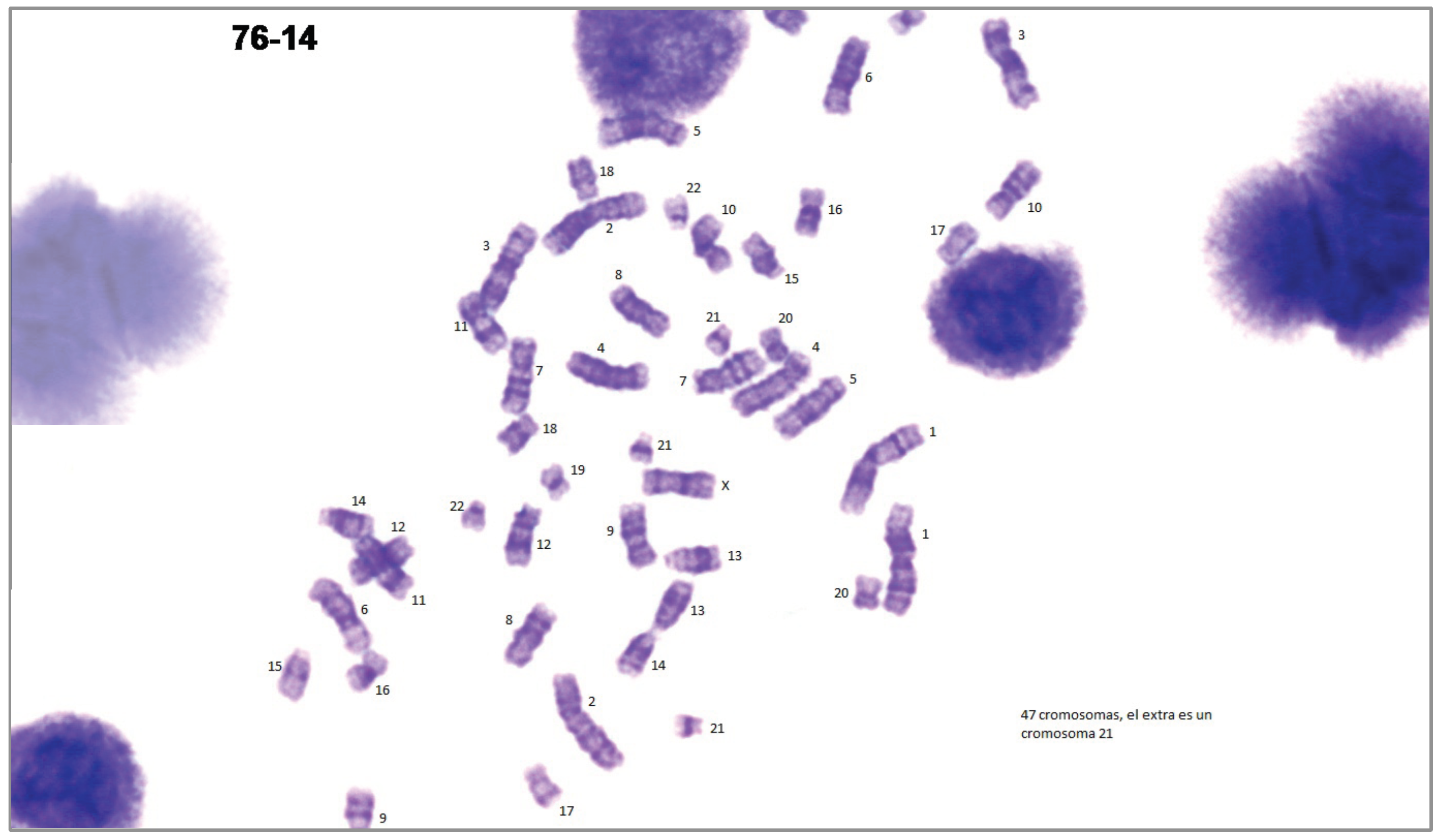
• A dataset obtained in collaboration with cytogeneticists of the CHT. The database consists of 24 G-banded prometaphase images acquired from 24 different patients and their corresponding manual karyograms. This dataset is under construction, and results have not been published elsewhere. In order to use the data of the Laboratory of Cytogenetics of the CHT, the Research and Education Department of the CHT reviewed and approved the use of the karyotypes in this work, judging that no appreciable risks or ethical issues were encountered, since no personal data associated to the karyotypes were issued.
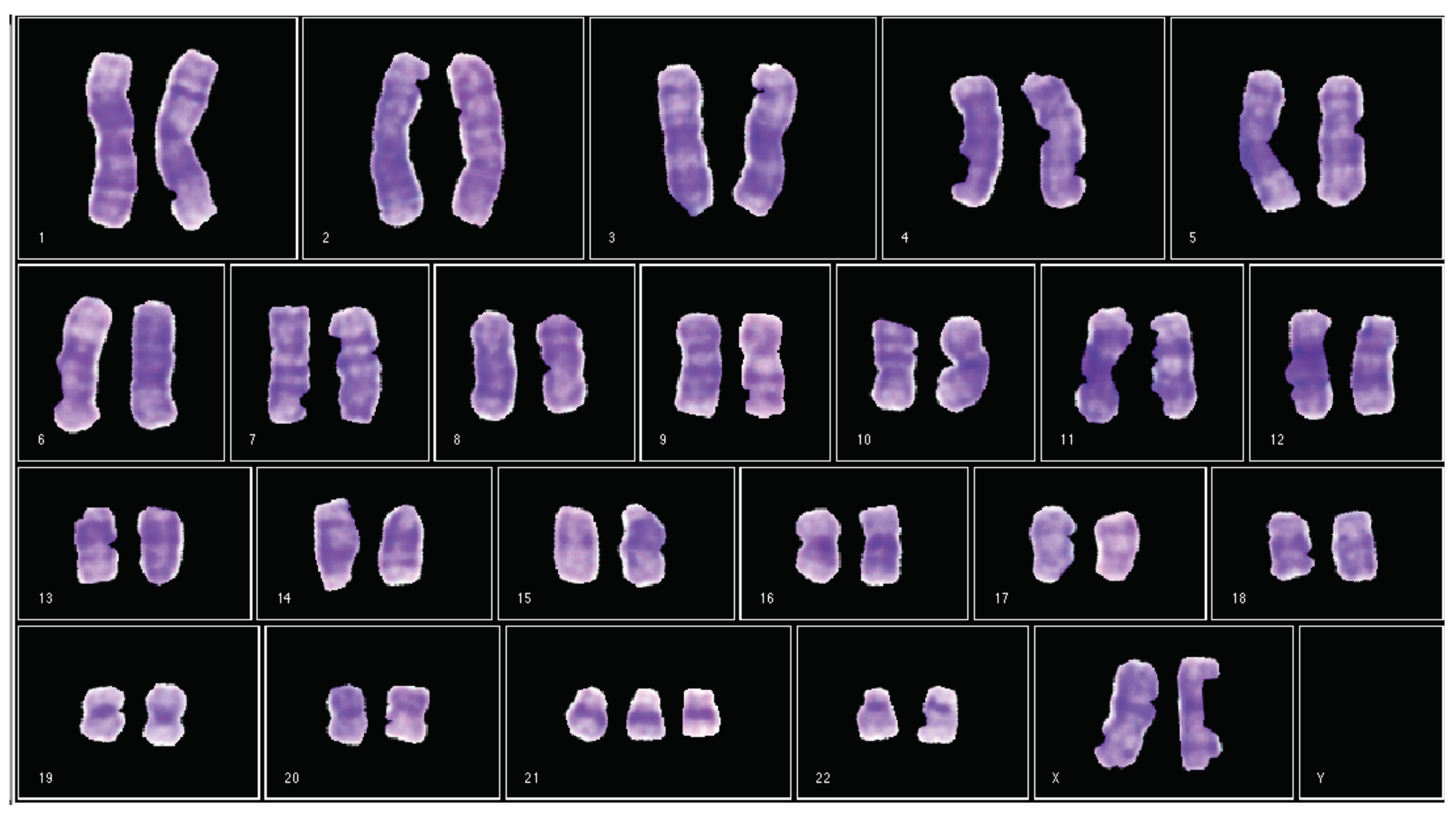
• A dataset retrieved from Laboratory of Biomedical Imaging (BioImLab) from the University of Padova. The database consists of 119 Q-banded prometaphase images and their corresponding manual karyograms acquired from the same number of cells [38].

To evaluate the proposed two-stage classifier scheme and to implement the desktop application for semi-automatic chromosome classification, the following software tools were used:

• Matlab R2014 has been used for the preprocessing, segmentation and transformation required in order to separate the chromosomes from the input prometaphase image. This software was alsa used to test multiple MLPs with several neurons in the hidden layer in order to find the optimal network configuration that yields the best performance.
• Weka 3.6.7 has been used to train and test classifiers selected for the comparison reported in this work.

To acquire the microscope images and evaluate the machine learning algorithms reported in this work, the following hardware tools were used:

• A Carl Zeiss Axioscope A1 microscope.
• An Axiocam ICC1 camera coupled with the microscope, with USB interface.
• A gateway desktop PC with Intel Core-2 Duo processor, 4GB RAM, and Linux 64-bit Mint OS.

2.2. Methods

The classification presented in this work is a part of a sequential process to automatically build a cytogenetic report. Figure 3 shows the required steps to generate this report. The first two steps are related to the chromosome segmentation and feature extraction, which were performed using a semi-automatic tool programmed for this purpose. This tool uses geometry and image processing techniques related to pixel labelling to perform these tasks. The segmentation and feature extraction process is planned to be presented in another paper. This paper is focused on the third step, related to the chromosome classification based on two main stages: a coarse classification where each chromosome is classified in one of three main groups; and a fine classification, where each chromosome in the coarse classification is assigned to one of the 24 chromosome types. Finally, the classification results are used to build the final karyogram.This tool is not addressed in this work

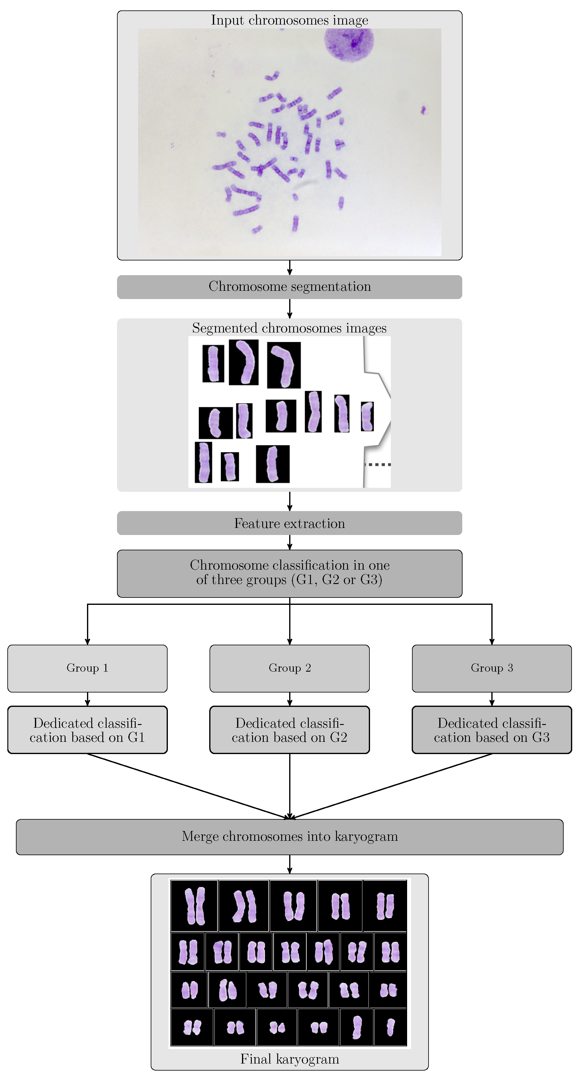
2.2.1. Outline of the Proposed Automatic Classification

To build the multistage classification described in the step 3 of Figure 3, five phases were conceived. Phases 1 to 4 are related to the construction of the classification model, while phase 5 is related to the development of a GUI that integrates the steps presented in Figure 3. Figure 4 shows the required phases to generate a classification model and build a karyogram.

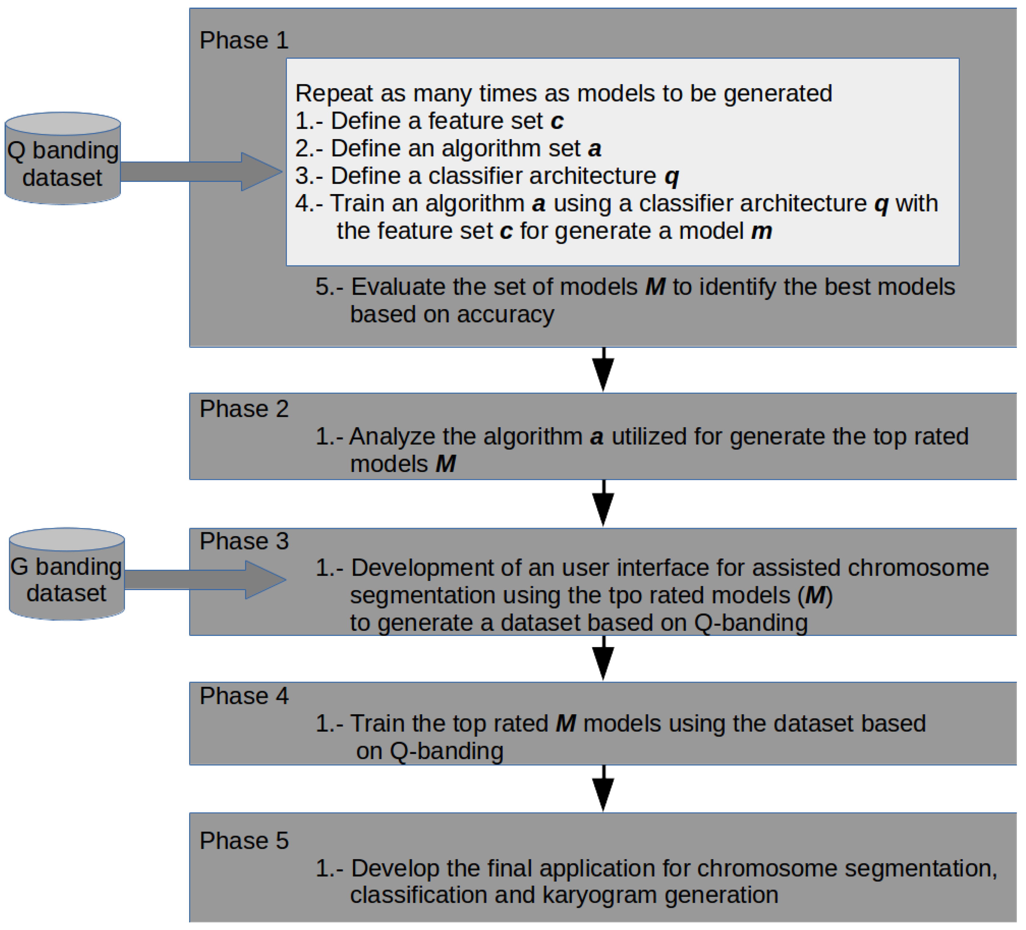
Phase 1. Classifiers Training

During this phase, a set M is generated, whose elements are the classification models, m, that were constructed to classify the chromosome images. $m_n$ is an element of the set M, that is $m\in M$. In this sense, m is composed of features, algorithms and architectures. $m_n$ is defined as $m=(c_i,a_j,q_k)$, where $c_i$ represents the features, $a_j$ the algorithms, and $q_k$ the architectures.

Features. The elements of the set C are the extracted features from the segmented chromosomes images. In this way, $c_i$ is a subset of the set C, where i is the index of the current subset. In

Table 1. Subset of features $\{c_1,c_2,c_3,c_4\}\subseteq C$.

Set		Description	Normalized
$c_1$		32 intensity values along medial axis	NO
$c_2$		32 intensity values along medial axis	YES
$c_3$		Perimeter Area Medial axis length Intensity levels along 64 traversal lines touching the medial axis Length of 64 traversal lines touching the medial axis	YES
$c_4$		Perimeter Area Medial axis length	YES

, the features used in each element of the C set are described.

Algorithms. The set of classification algorithms A, is composed of 51 algorithms found in the Weka (Waikato Environment for Knowledge Analysis) platform. Hence, $a_j$ represents the subset of algorithms, where $a_j\subset A$, and j is the current algorithm.

Table 2. Subset of classification algorithms $\left\{a_1\right\}\subseteq A$.

1 BayesNet	27 NNge (Non-Nested generalized exemplars)
2 DMNBtext (Discriminative Multinomial Naive Bayes)	28 OneR (1-R classifier)
3 NaiveBayes	29 PART (Partial decision trees)
4 NaiveBayesMultinomial	30 Ridor (RIpple-DOwn Rule)
5 NaiveBayesMultinomialUpdateable	31 ZeroR (0-R classifier)
6 NaiveBayesSimple	32 BFTree (Best-First decision tree)
7 NaiveBayesUpdateable	33 DecisionStump
8 IB1 (Instance-based classifier)	34 FT (Functional Trees)
9 KStar	35 J48 (C4.5 Decision Tree)
10 LWL (Locally Weighted Learning)	36 J48graft (Decision Tree Grafting)
11 AdaBoostM1	37 LADTree (LogitBoost Alternating Decision Tree )
12 AttributeSelectedClassifier	38 RandomForest
13 Bagging	39 RandomTree
14 ClassificationViaClustering	40 REPTree (Reduced-Error Pruning)
15 ClassificationViaRegression	41 SimpleCart
16 CVParameterSelection (Cross-Validation)	42 Logistic
17 END (Ensembles of Balanced Nested Dichotomies)	43 MultilayerPerceptron
18 FilteredClassifier	44 RBFNetwork (Radial Basis Function Network)
19 Grading	45 SimpleLogistic
20 LogitBoost (Additive Logistic Regression)	46 SMO (Sequential Minimal Optimization)
21 MultiBoostAB (Ada Boost)	47 DTNB (Decision Table/Naive Bayes hybrid)
22 MultiClassClassifier	48 Dagging
23 MultiScheme	49 Decorate (Diverse Ensemble Creation)
24 HyperPipes	50 LMT (Logistic Model Trees)
25 VFI (Voting Feature Intervals)	51 NBTree (Naive-Bayes Tree hybrid)
26 JRip (Repeated Incremental Pruning)

summarizes the algorithms from set $a_1$.

Table 3. Subset of classification algorithms $\left\{a_2\right\}\subseteq A$.

1 IB1 (Instance-based classifier)

2 KStar

3 Random Forest

4 Multilayer perceptron

5 SMO (Sequential Minimal Optimization)

summarizes the top rated algorithms $a_2$ obtained at the end of phase 1.

Architectures. The set Q is composed of binary and multiclass architectures used in the classification. In this way, $q_k$ represents a classification architecture, where $q_k\subset Q$, and k is the index of the current architecture.

Table 4. Subset of architectures $\{q_1,q_2,q_3,q_4\}\subseteq Q$.

Set	Type	Outputs	Description
$q_1$	Multiclass	24	Classify chromosomes into 24 classes
$q_2$	Multiclass	3	Classify chromosomes into 3 groups
			G1: Chromosomes from 1 to 7
			G2: Chromosomes from 8 to 15
			G3: Chromosomes from 16 to 24
$q_3$	Binary	6	3 binary classifiers are included:
			BG1: Chromosomes belongs to G1 or not
			BG2: Chromosomes belongs to G2 or not
			BG3: Chromosomes belongs to G3 or not
$q_4$	Multiclass	24	3 multiclass classifiers are included:
			MG1: Chromosomes from 1 to 7
			MG2: Chromosomes from 8 to 15
			MG3: Chromosomes from 16 to 24

summarizes the algorithms from sets $q_1$ and $q_2$.

As depicted in Figure 4, phase 1 is divided into 5 activities. The first 4 activities are repeated as many times as the number of the required classification models, $m_n$. In the activity number 5, the best element of the set M is selected. These activities are described below:

1.

From the literature, groups of features that can be extracted from Q-band chromosome images where formed. These were listed as the subset of features $c_1$, $c_2$, $c_3$, and $c_4$ and are presented in Table 1. In this activity, one of the feature groups $c_i$ is selected to be extracted from every chromosome in the image database. With these features, two sets are generated in separated datasets to be utilized in training. The first dataset is used to train the classifiers and the second one as test dataset.

2.

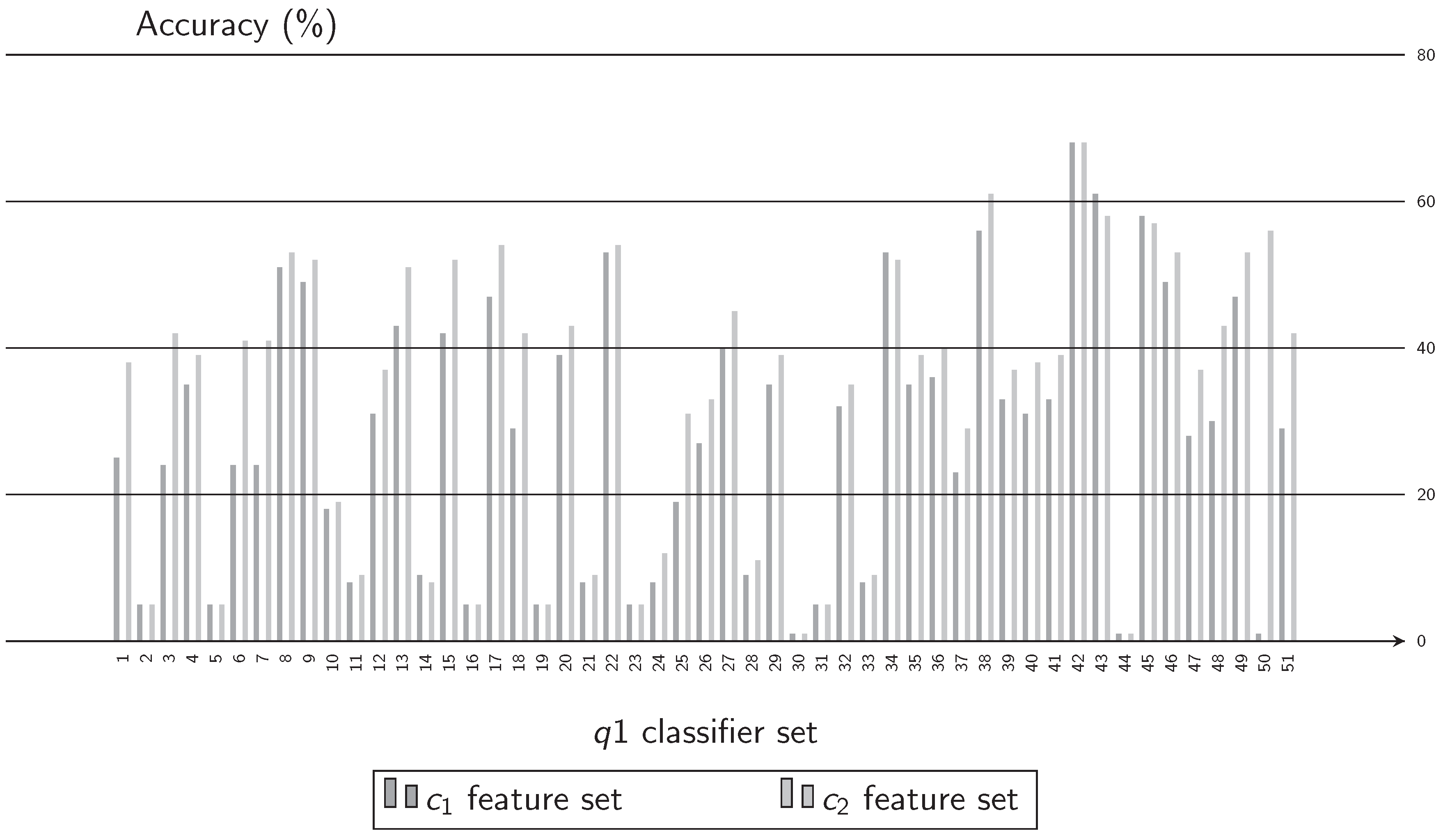
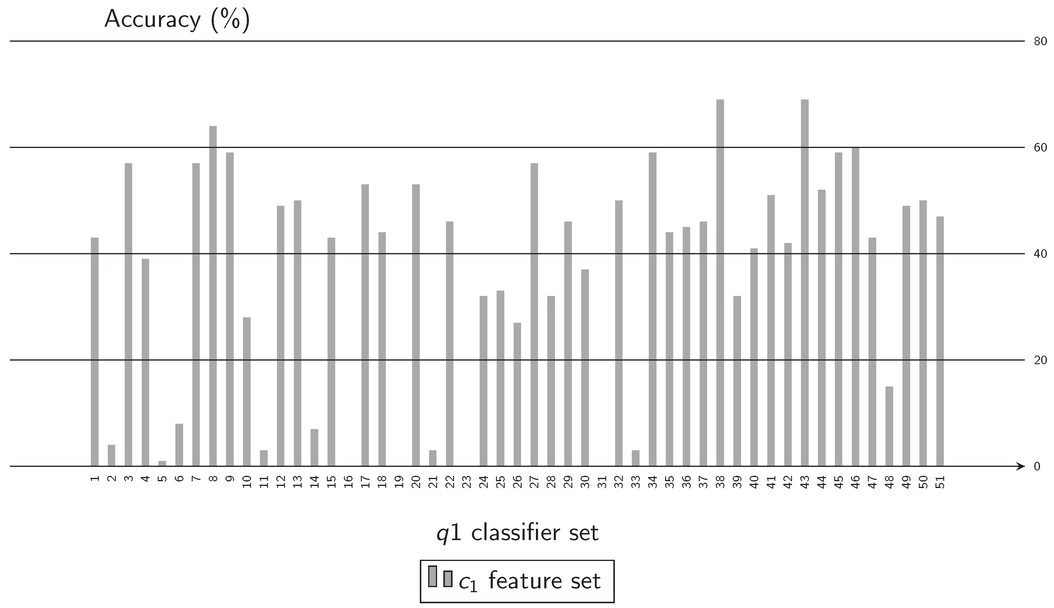
In this activity, a group of classification algorithms available in the Weka platform is selected and identified as the set A. These elements conform the subset $a_1$. According to the experimental results, the elements of the subset $a_1$ were modified to form the subset of algorithms, $a_2$. The algorithms of subset $a_1$ are enlisted in Table 2, and for subset $a_2$ in Table 3.

3.

This activity defines the architectures that will be used in chromosomes classification. An architecture $q_n$ represents how the chromosomes are going to be classified in one of the 24 output classes. For example, one architecture could be a multiclass classification, where the chromosome would be assigned directly to 1 of the 24 classes. Another option is to divide the group into autosome and sex chromosomes, and identify if it belongs to one of this groups or not (binary classification). Table 4 summarizes the defined architectures for this activity.

4.

Training and testing of a model $m_n$ is performed in this activity. The training and testing dataset, the set of algorithms $a_j$ and the classification architecture $q_k$ are the elements of the current model, $m_n$. The training and testing accuracies are reported, and they are used as evaluation metric for the next activity.

5.

Once several models were generated (through activities 1 to 4), the best chromosome classification model, $m_n$, is identified, based on the chromosome classification accuracy. Current $m_n$ could represent, either the output of phase 1, or the final classification model, m.

Phase 2. Classifier Analysis

In this phase, the algorithm $a_j$ from the classification model m obtained in phase 1 is analyzed in order to find a relationship between the results and the configuration of this algorithm. This is an intermediate phase to integrate the selected classifier to the next phase.

Phase 3. Application Development

Here, a GUI is developed to allow the cytogenetist to use a semi-automatic tool to segment the chromosomes in G-band images. Then, the segmented chromosomes are used to build the G-band image database. This tool is also used to extract the chromosome features defined in the classification model, m, that was obtained as a result of phase 1.

Phase 4. Classifiers Training

During phase 1, a classification model, m, was obtained by training the algorithms $a_j$ using the Q-band image database. In this phase, the algorithms $a_j$ are trained again, following the classification architecture $q_k$ obtained in phase 1, but this time using the features extracted from the G-band chromosome images. To validate each model the k-fold cross validation is used with a k = 10.

Phase 5. Application Integration

In this phase, an application consisting of 3 modules, named A, B and C, was developed.

Module A: 

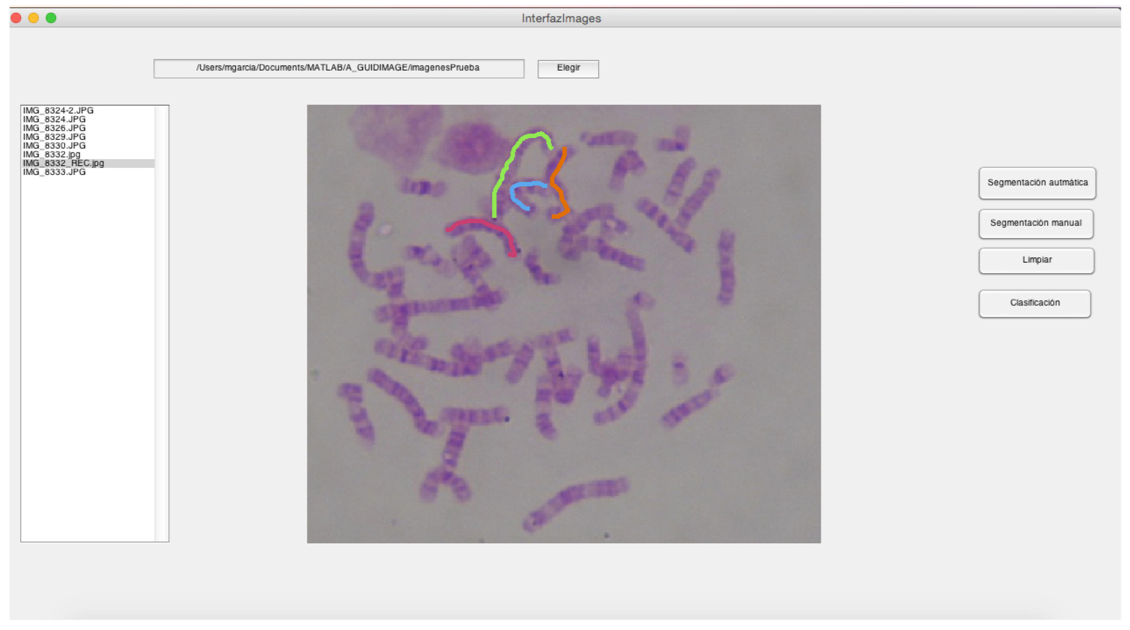
This module includes a GUI and the segmentation related operations. It allows the user to generate the segmented chromosomes and arrange them in directories.

Module B: 

It comprises the automatic classification operations, including the development of a GUI that allows the user to: (i) Enter the segmented chromosomes obtained by the module A; (ii) Use the classification model m, obtained in phase 4. Its output is composed of the classified chromosomes.

Module C: 

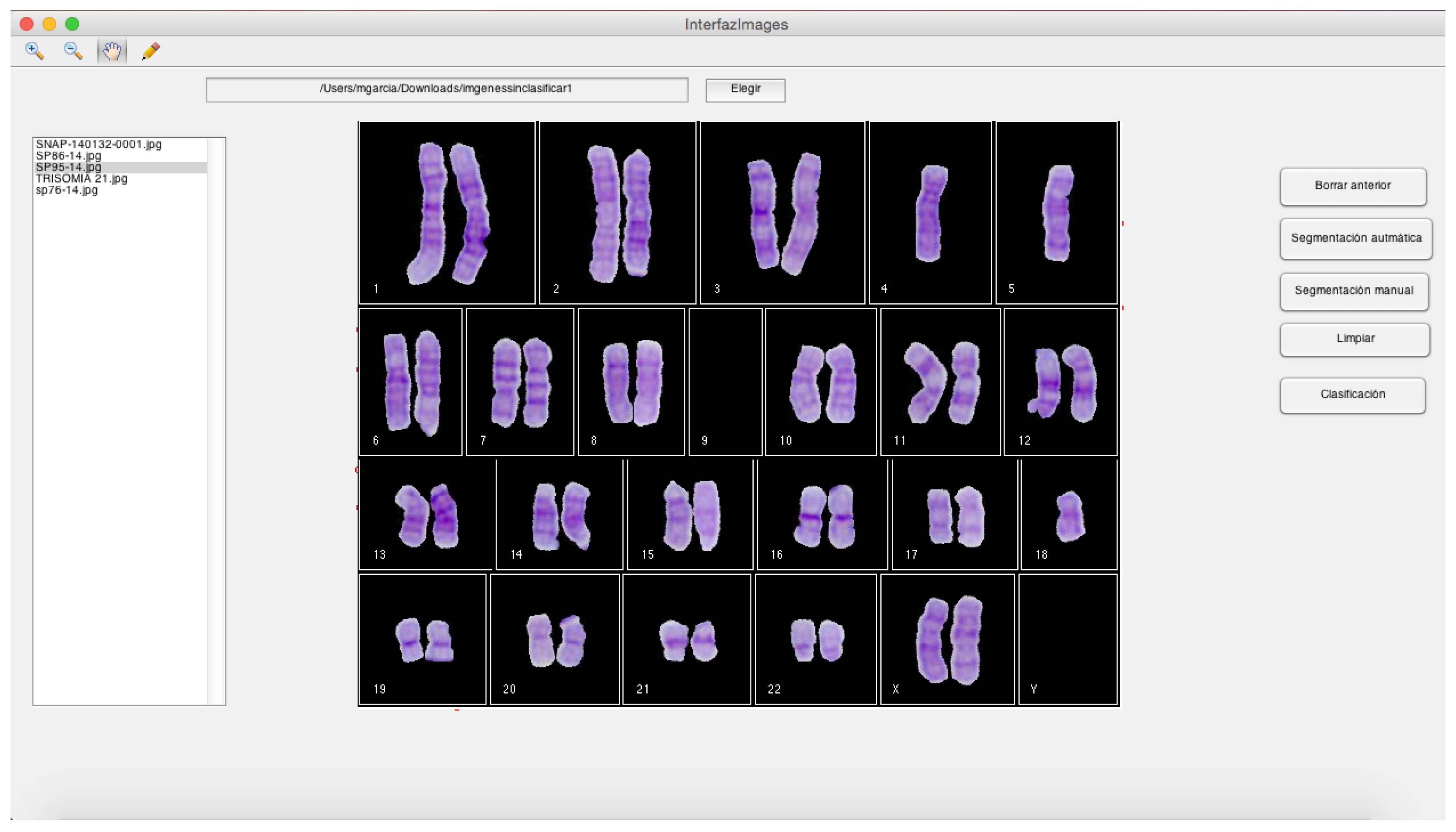
It is a GUI that generates a karyogram using the classified chromosomes obtained in module B. This karyogram is interactive, since the module allows the user to change the chromosome polarity and its membership class. In addition, this module generates a cytogenetic report in the format defined by the cytogeneticist.

3. Results and Discussion

Results presented in this section are reported according to the stages previously described. Four experiments were performed in order to identify the best classification algorithm for the aimed application. Two more experiments were carried out to find out the feature set that best describes the chromosome in the context of automatic classification.

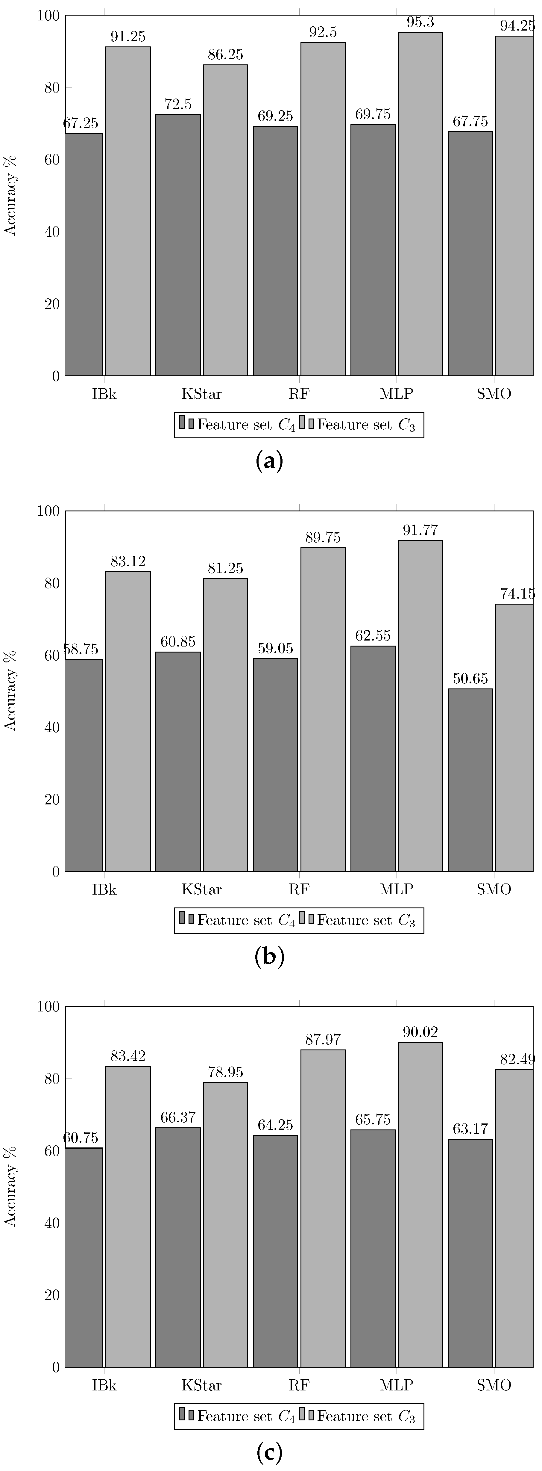
3.1. Experiment 1. Feature Selection

Results of this experiment will yield the features that best describe the chromosomes and the related accuracy for each tested feature set. For a first training round, the set of algorithms $a_1$ and the group of features $c_1$ were used, along with a multi-class architecture, $q_1$, where the chromosomes were classified in classes from 1 to 24. In this experiment, the highest accuracy was 60.80%, obtained by the Random Forest (RF) algorithm. The rest of the tested classification algorithms achieved a classification accuracy under 57%. The experiment was repeated with the normalized version of $c_1$ features (set $c_2$). Results show that the Multilayer Perceptron (MLP) artificial neural network (ANN) obtained an accuracy of 60.72%. During the first round of this experiment, the accuracy of the RF algorithm was 0.08% greater than that of the MLP algorithm. In the second round, when using $c_2$ set (normalized data), all the classification algorithms obtained better results, except the RF. In Figure 5, the accuracy for $c_1$ and $c_2$ feature sets are compared.

This experiment did not yield the optimal feature set to describe the chromosomes, although its results shown that the feature vector must be normalized in order improve the accuracy in 98% of the tested algorithms. In the other hand, though this experiment, the training time for each classifier could be measured. The training time of the 51 classifiers, using 32 features on the selected hardware, took at least 24 h for each classifier, and thus it was proposed to reduce the number of algorithms to be tested, in order to work with the algorithm that obtained the best results in the shortest time.

In this experiment, accuracy results from the models generated with reduced feature sets are lower (60%), compared to the models where the full set of features is used. This indicates that feature selection and reduction would not improve the obtained results when the full set of features was used.

3.2. Experiment 2. Training Time

The purpose of this experiment is to reduce the number of classifiers to test, by identifying and keeping those yielding the best results for the experimental data set.

For the next tests, the feature set $c_3$ and the multi-class architecture $q_1$ were used. In the first round, where 10 chromosome images were used, the best classification accuracy, 64.73%, was obtained by the MLP classifier. In order to identify the classifiers yielding an similar accuracy compared to the MLP classifier, the classifiers with an accuracy above 60% were selected to conform the set of classifiers $q_2$, as shown in Figure 6. The set $q_2$ is presented in Table 2. Next, using the set of 119 images, the best accuracy was obtained by the same classifier (MLP): 86.77%. The accuracies obtained in this experiment are reported in Figure 7.

In these experiments, 51 algorithms were tested and 5 of them obtained accuracies above 60%. The selection of the 60% threshold is arbitrary, considering that a 50% accuracy is not better than a random classification. The accuracy obtained in this round of experiments was used to discard the algorithms with worse accuracies for our purpose and to reduce the training time in future experiments. It is worth noting that during the second round of this experiment, more training information was used, rising the execution time, but improving the classification accuracy results, from 67.58% to 86.78% when using the MLP algorithm. Figure 7 shows the classifiers that yielded the best accuracies. Results of this experiment show that the MLP classifier yielded the best accuracies and could be used in the final classification model.

Execution time was not studied, but results showed that between 5 and 7 s are needed to classify a whole set of chromosomes once the trained model was obtained.

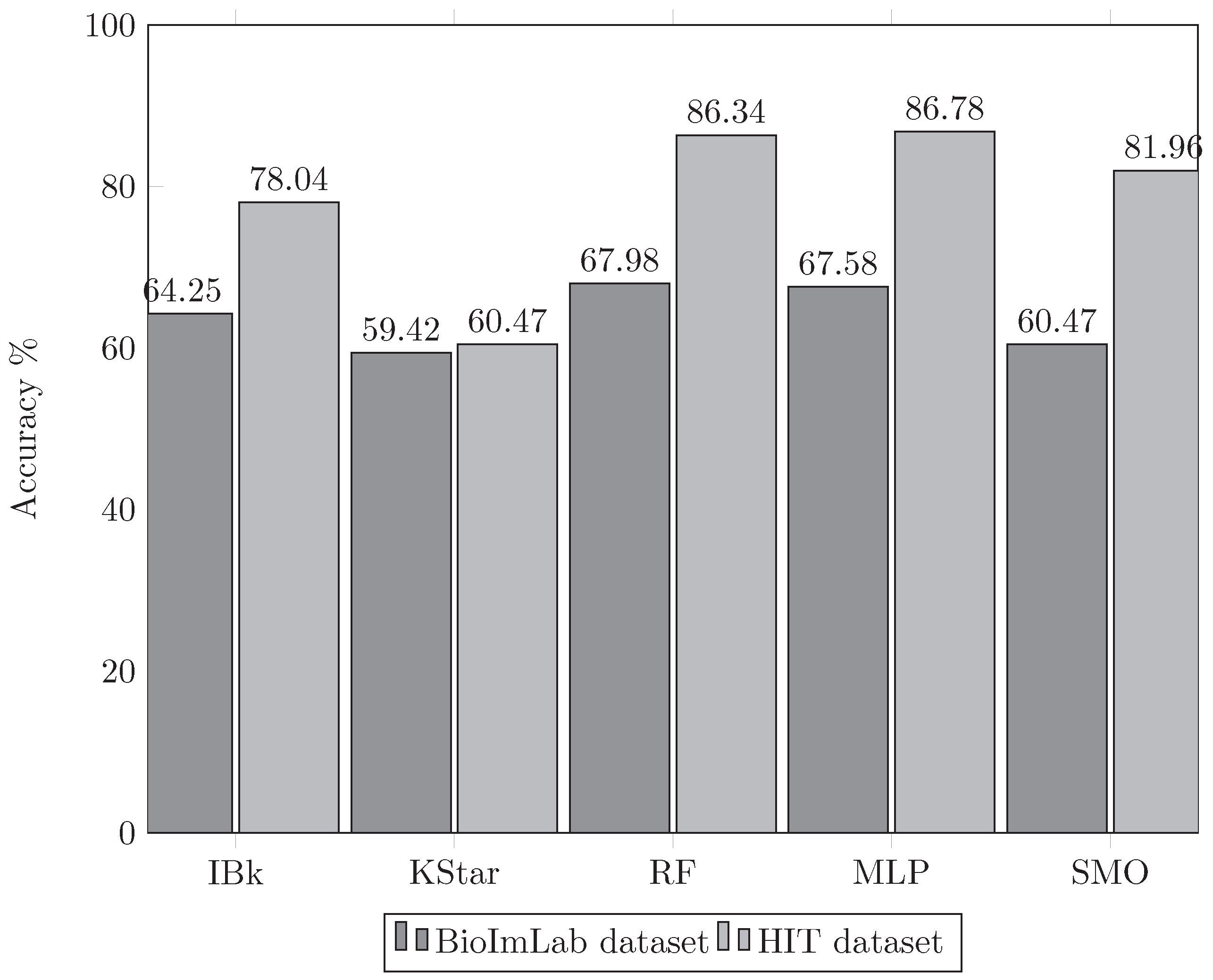
3.3. Experiment 3. Two Stage Classification

Once that the classifiers yielding the best accuracy were identified as the set $q_2$, in this third experiment the classification process was divided into two stages. This division is depicted in Figure 3. In the pre-classification stage, the objective is to segregate the chromosomes into wide groups, and use this output as the input of a final classification into 24 classes. In Reference [39], the authors propose applying a post-classification process to re-assign a chromosome to a different class when a wrong number of chromosomes is found in some class. In this work, a post-classification process is executed to reassign the misclassified chromosomes to their correct class.

According to the International System of Human Cytogenomic Nomeclature (ISCN) [40], chromosomes can be grouped by shape and area. In Reference [25], the authors propose a hierarchical classification approach, where they divide the chromosomes into seven groups. For the G-band chromosomes images used in this work, this preclassification into seven groups gave accuracy results lower than the single phase classification. It was found that the preclassification in three groups worked better for the G-band dataset, then the pairs are divided as followsThe 3 pre-classification groups are defined according to the shape and area of the chromosome. The 23 chromosome pairs are divided as follows:

• Group 1: Chromosomes 1 to 7.
• Group 2: Chromosomes 8 to 15.
• Group 3: Chromosomes 16 to 23.

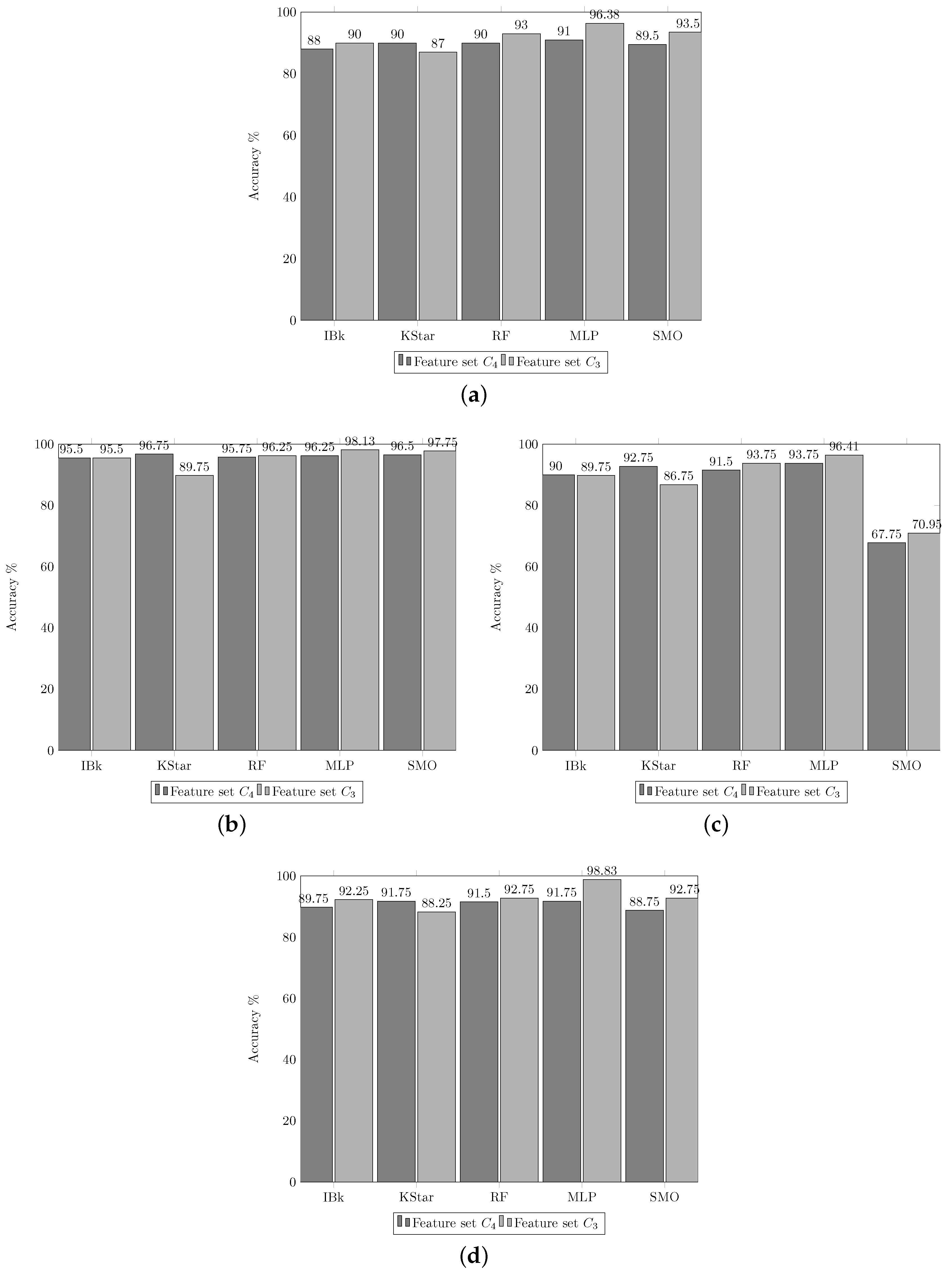
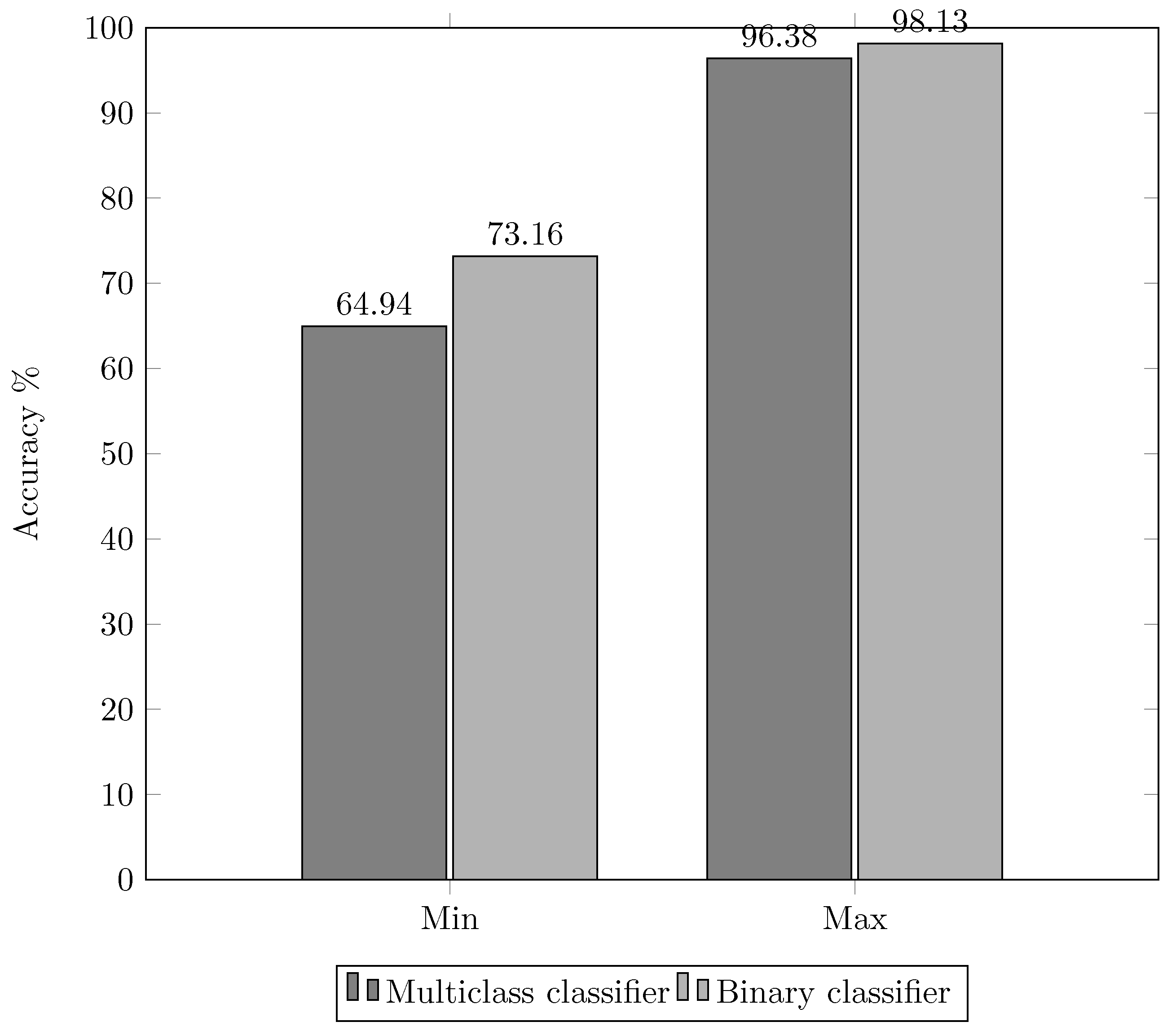
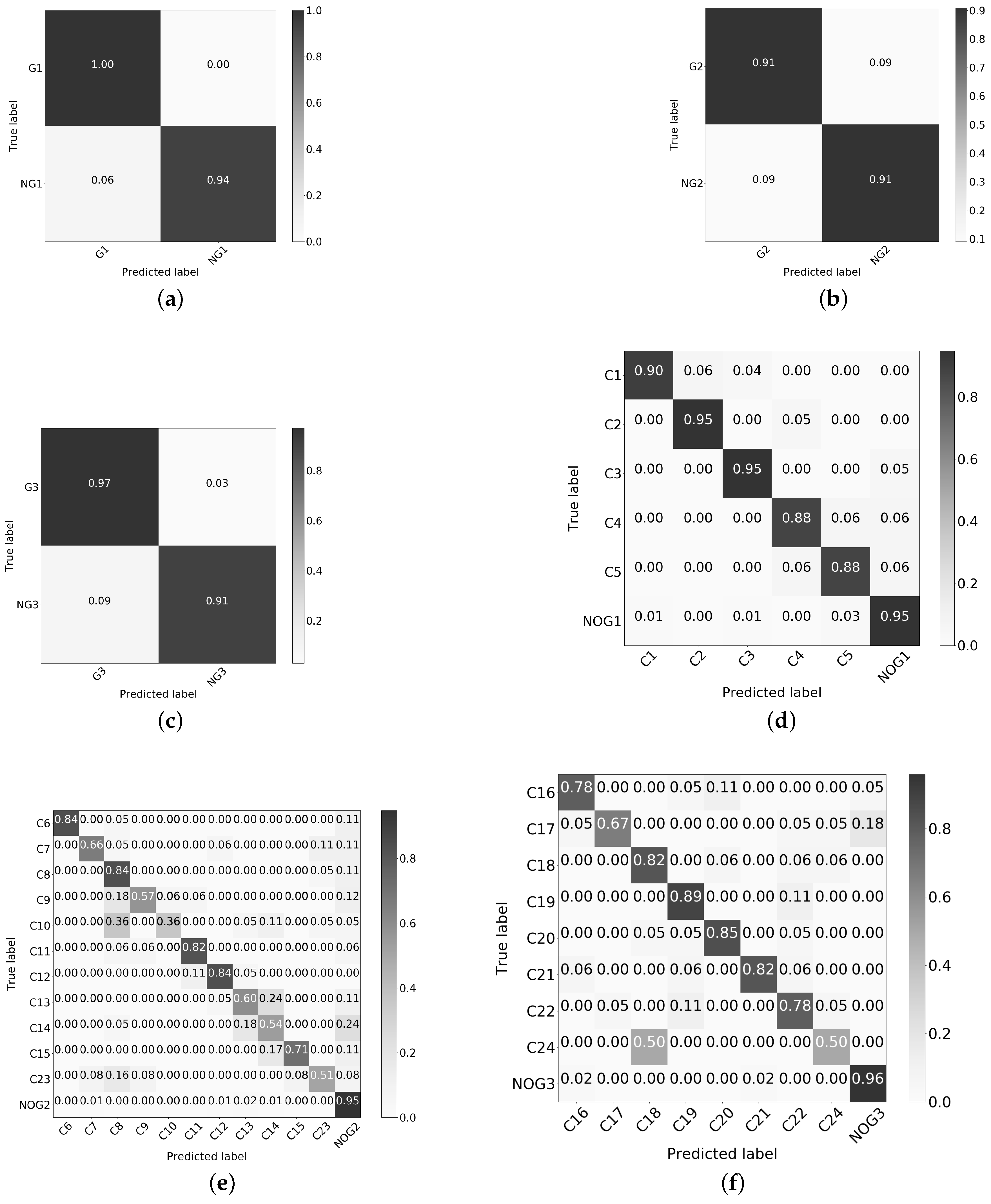
3.4. Pre-Classification Stage

This stage could be performed using two types of architectures: multi-class and binary, which are explained below:

1.

Multi-class ($q_2$ architecture). Two groups of features, $c_3$ and $c_4$, are used to decide if the current chromosome belongs to one of the three groups.

2.

Binary ($q_3$ architecture). The groups of features, $c_3$ and $c_4$, are used to decide if a chromosome:

(a)

Belongs to group 1 (G1) or does not belong to group 1 (NOTG1).

(b)

Belongs to group 2 (G2) or does not belong to group 2 (NOTG2).

(c)

Belongs to group 3 (G3) or does not belong to group 3 (NOTG3).

Figure 8a shows the results of the multi-class classifiers. The accuracy for all these classifiers was close to 90%. In the other hand, the results of the binary classifiers are shown in Figure 8b–d, where it can be observed that most of the tested classifiers obtained accuracies close to 90%, except the SMO classifier in group 2, where non-optimized hyperparameters were used. In the other hand, the results of the binary classifiers are shown in Figure 8b–d, where it can be observed that all of the classifiers obtained accuracies close to 90%. Although, the best results were obtained using the $q_3$ architecture (binary classification) and the feature set $c_3$. It is worth noting that classifier with the best accuracy was the MLP.

The purpose of this experiment was to pre-classify the chromosomes into three different groups, working with the feature sets $c_3$ and $c_4$. The group $c_3$ is a vector of 131 features, while the group $c_4$ is conformed of only 3. It was observed that the best results were obtained using the feature set $c_3$, both in the binary and multiclass classifiers. The binary and multiclass classification schemes were compared using the MLP classifier, since it gave the best results in both schemes. The minimum and maximum accuracies of both schemes are compared in Figure 9. The minimum and maximum percentages for the binary scheme are 73.16% and 98.13%, while the results for the multi-class scheme are 73.10% and 64.94%, respectively. This test showed that the binary classifiers obtained higher accuracies.

3.5. Post-Classification Stage

In this stage, the pre-classification into 3 groups scheme was applied over the same training set in the same way as in phase 2, but using this time a reduced multi-class classification scheme with the feature sets $c_3$ and $c_4$.

Figure 10 presents the results of this experiment, where once more time, the best results are obtained using the feature set $c_3$ and the MLP algorithm, obtaining accuracies of 95.30%, 91.77% and 90.02% for the groups 1, 2 and 3, respectively.

Once the chromosomes were classified into 3 wide classes, the next step was to use this classification as the input of a multi-class classifier. The highest accuracies were obtained by the MLP classifier, being 95%, 91% and 90%, for the groups 1, 2 and 3, respectively.

Finally, the performance of the whole classification scheme was tested by a complete classification round, creating a dataset containing every testing sample. When the same sample was assigned to two different classes during the phase 1, its final class was reassigned according to the highest membership percentage. Once the classification into three wide classes was obtained, the Phase 2 was carried out, using the multi-class algorithms over 24 classes, where 76.44% of the whole set of chromosomes was correctly classified.

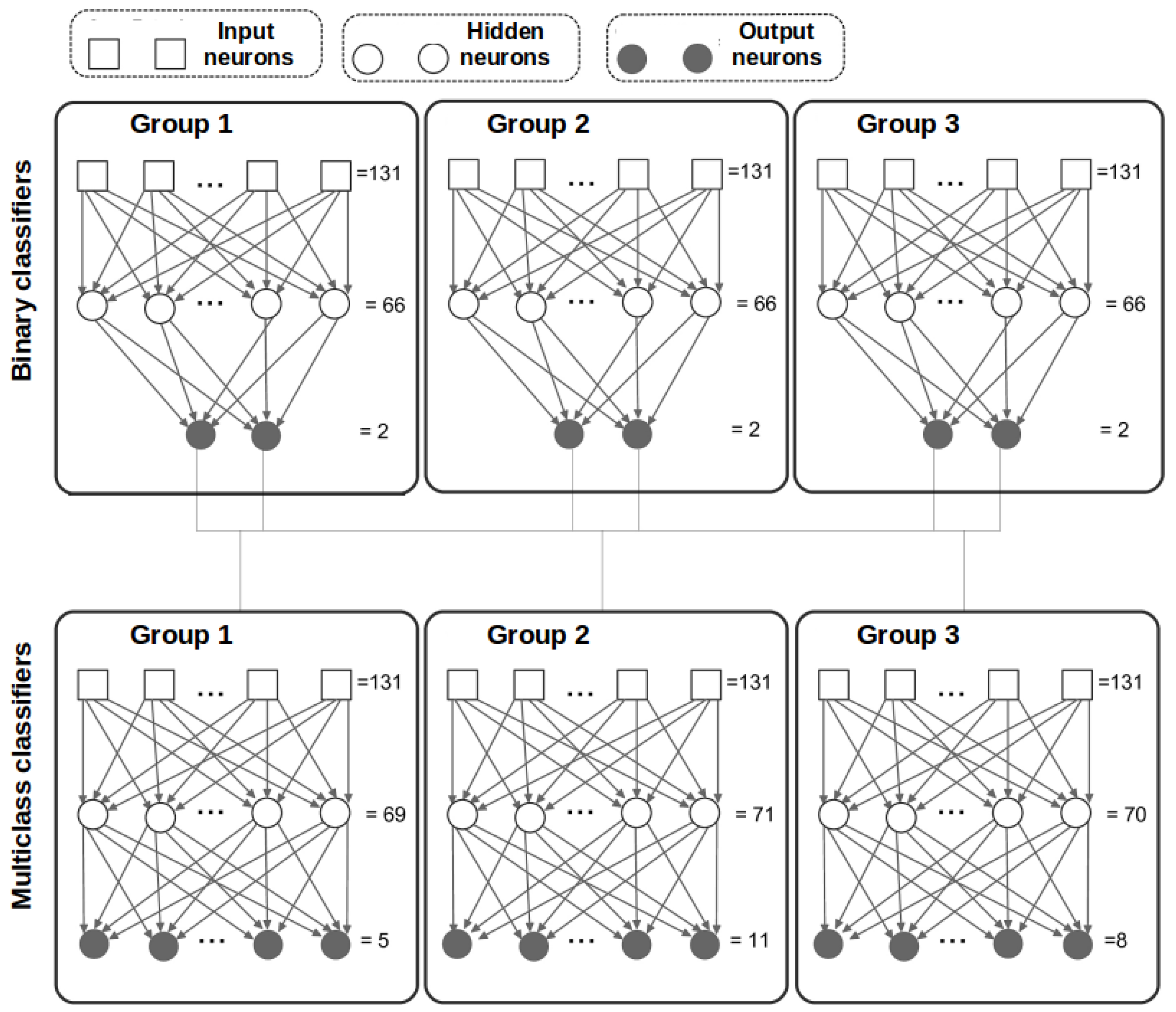
3.6. Experiment 4. Redefinition of the 2 Stage Classification

In experiment 3, in the pre-classification stage, accuracies above 90% were obtained using the following configuration; the 90% accuracy threshold was selected observing that the maximum accuracy reported in the literature was 94% in the work in Reference [26] using a refined ANN. In the present work it was decided to round this value to the nearest ten below, since a non-refined ANN is being used:

• Feature group $c_3$;
• MLP classifier; and
• $q_3$ (Phase 1, binary classifiers) and $q_4$ (Phase 2, multi-class classifiers) architectures.

In a new experiment, the same configuration was used, but this time the 3 wide groups were redefined during the training stage. This new group definition was based on the size characterization dictated by the System for Human Cytogenetic Nomeclature (ISCN) [40]. Changes to model previously presented in Figure 3, are shown in

Table 5. Redefinition of the initial two-stage model.

New Class	Chromosomes
	Model 1	Model 2
Group 1	1 to 7	1 to 5
Group 2	8 to 15	6 to 15 and 23
Group 3	16 to 24	16 to 22 and 24

.

In phase 1, the obtained accuracies were 99.49%, 97.85% and 98.64% for the groups 1, 2 and 3, respectively. In phase 2, the accuracies were 99.24%, 92.69% y 92.47% for the groups 1, 2 and 3. Results of experiment 4 are shown in Figure 11.

The results of the classification of the whole chromosome set using the modified model yielded a accuracy of 88.45%, which is higher than the result of the classification using the initial two-stage classification by 12.01%.

The classification algorithm used for this test was the MLP, that is an Artificial Neural Network (ANN). The default configuration of this algorithm in Weka is presented in Figure 12.

This configuration uses 6 ANN, with 131 neurons in the input layer, corresponding to the size of the feature set. The number of neurons in the hidden layer was defined as: $H{L}_{neurons}=(a+c)/2$, where a are the attributes and c the classes. Finally, the number of neurons in the output layer corresponds to the number of classification classes.

3.7. Application of the Proposed Model to the G-Band Images Dataset

The G-band image dataset (GID) is composed of 24 studies of chromosomes in metaphase. The dataset and its manual classification by an expert were provided by the laboratory of cytogenetics of the CHT. Using automatic and semi-automatic segmentation tools developed by our team, the chromosomes were individually segmented and a dataset of 1097 G-band chromosome images was composed. If the karyotypes were taken from healthy people, the total number of chromosomes of the dataset should be 1104, but some of the provided studies presented some anomaly in the number of chromosomes, for example, some studies lacked chromosome 4 or 18. It is worth noting that the number of elements of the G-band dataset is only 20% of that of the Q-band dataset. Figure 13 shows an example of the chromosomes in G bands.

The segmented GID was then used to train the ANN architecture presented in Figure 12. Using binary and multi-class classifiers, in phase 1, the accuracies were 95.26%, 90.56% and 93.6%, for the groups 1, 2, and 3, respectively. In phase 2, the accuracies were 91.12%, 77.08% and 84.4%, for the same groups. Finally, the overall accuracy was 80.99% for the whole set.

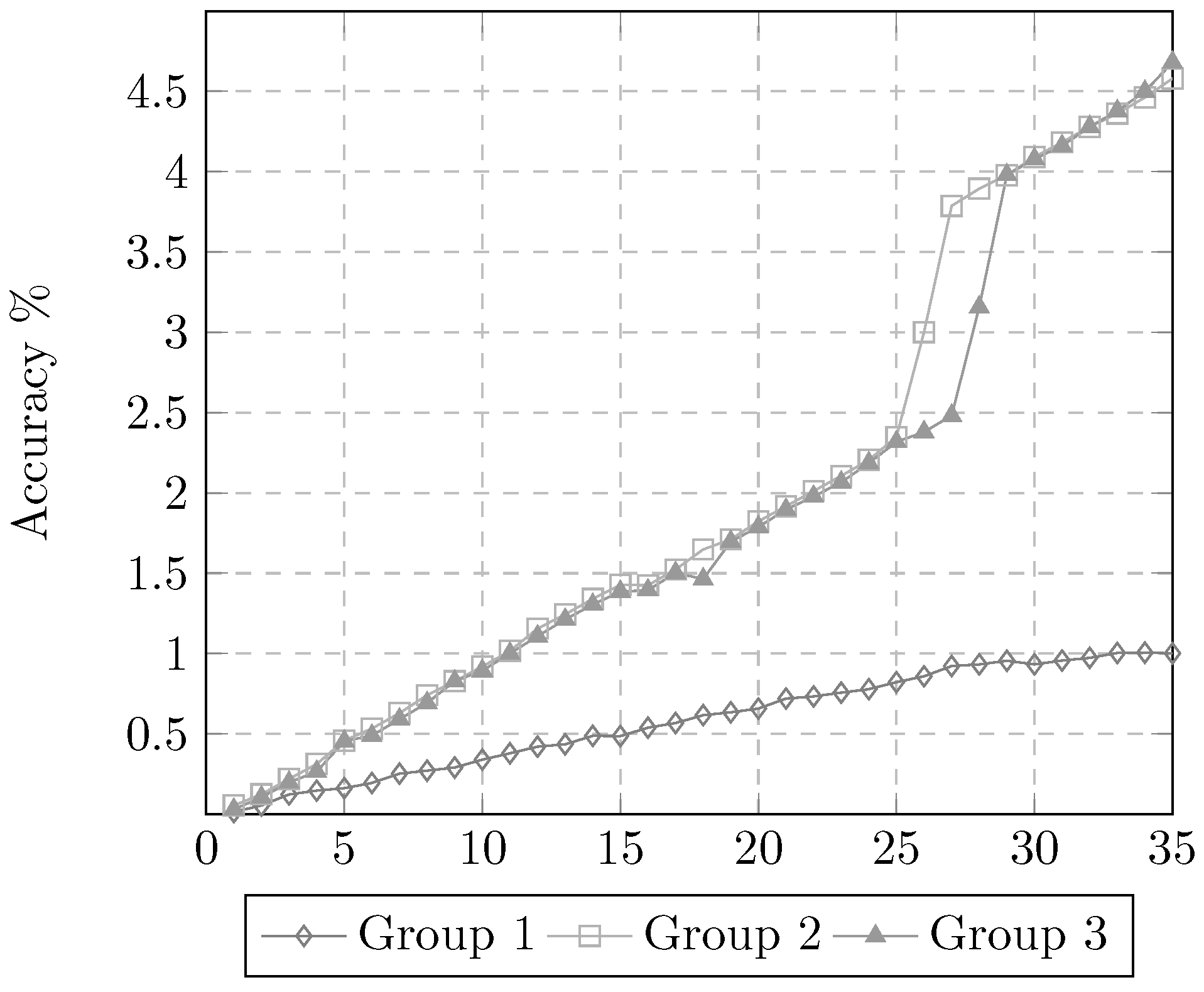
3.7.1. Changes in the Number of Neurons in the Hidden Layer

In order to improve the obtained accuracies in 3 wide classes for the GID, the number of neurons in the hidden layer of the ANN presented in Figure 12, was varied from 1 to the maximum number of neurons in the default configuration of Weka (70 neurons). The result of accuracy for the varying number of neurons is presented in Figure 14.

For the phase 1 binary classification, the highest accuracies were 94.71 %, 89.56% and 92.7%, for the groups 1, 2 and 3, respectively. In phase 2, the obtained percentages were 91.71 %, 76.51% y 86.4%, for the same groups. Using this new configuration, the overall accuracy was 82.36% for the whole set.

Table 6. Summary of best classification accuracy versus hidden neuron number.

	Original Configuration		Modified Configuration
	Binary Classification
Group	Neurons	Accuracy	Neurons	Accuracy
1	66	95.26	4	96.44
2	66	90.56	20	90.29
3	66	93.60	34	93.60
	Multiclass Classification
1	68	91.12	17	92.89
2	71	77.08	67	79.24
3	70	84.40	30	86.40

, summarizes the tested number of neurons in the hidden layer for each classifier, and their corresponding classification results.

It is worth noting that the accuracy of classification do not show a radical change when using less neurons. For example, in the case of the group 1, when using binary classifiers and varying number of hidden-layer neurons form 1 to 70, the classification results were between 94% and 95%; and for the rest of the groups the observed behavior was similar. This fact is important because if the high classification results persist even using less neurons, the training and evaluation times are reduced, without affecting the functionality of the classifier. Figure 15 shows the mean time for training a classifier. This test was carried out on computer with an Intel Core Duo 2, 4 GB of RAM memory, running Linux Mint operating System. This plot shows only 35 form 70 iterations, because the rest of the tests were done over different computers. The training time increases as more neurons are used, although the classification accuracy results are preserved.

3.7.2. Validation of the ANN Models

Figure 16 shows the confusion matrices for the MLP-ANN that obtained the best accuracy in both stages of the proposed system. For each group, a confussion matrix with the false positives (FP), false negatives (FN), true positives (TP), and true negatives (TN) is shown. In Figure 16a–c, the confussion matrices for the first classification stage are shown. The lower accuracy was found in the group 2, where a 0.91 accuracy is obtained. In Figure 16d, the confussion matrix has a minimun accuracy of 0.88 for chromosomes C4 and C5. In Figure 16e, the minimum obtained accuracy is 0.51 for the class C23. Finally, in Figure 16f, the lower accuracy is 0.5 for the class C24. The group that exhibits the lowest accuracies is the group 2 of the multi-class classification, where most of the tested classifiers have scores below 60%. Finally, the chromosome number 10 presented the lowest accuracy (35%).

In this section an ANN two-stages classification model applied to G-band chromosomes images was proposed. This model obtained a accuracy of 88.45% over a Q-band image dataset. The same model attained a percentage of 82.02% when it was applied over a G-band image dataset. It is worth noting that the G-band dataset was composed of only 24 karyotypes, while the number of karyotypes of the Q-band dataset was 119. A classification model trained with more information will obtain better results.

A two-stage classification scheme was proposed. In the first stage, the chromosomes are classified in 3 wide groups, based on the ISCN length characterization of chromosomes. In a second stage, the output of the first stage is used as input for a multi-class classifier applied over each wide class. This allowed us to improve the accuracies. The ANN used in this scheme was tuned by reducing the number of neurons in the hidden layer without affecting the final classification result.

3.7.3. Desktop Application for Semi-Automatic Chromosome Classification

In Figure 17, a screenshot of the developed semi-automated chromosome segmentation desktop app is shown. The cytogeneticist can read chromosome images from the microscope connected to the computer that hosts the desktop application. Once the chromosome image has been acquired, the cytogeneticist can choose between two segmentation modes: the automatic or the semi-automatic mode. In the semi-automatic mode, the cytogeneticist interacts with the app by manually selecting the approximated medial axis to aid the segmentation process of the displayed chromosomes. The segmented chromosome are then automatically classified by the previously trained two-stage classifier to generate a preliminary karyotype with the classification label for each chromosome.

The cytogeneticist would use the generated results to build the final karyogram, including the possibility to manually correct misclassified chromosomes. In Figure 18, an example of a preliminary karyogram is shown. This karyogram is the output generated by the proposed system, and may need additional intervention of the cytogeneticist. In this specific situation, the misclassified chromosomes must be manually arranged by the cytogeneticist to have the final karyogram complete.

4. Conclusions

Most of the works in the literature about chromosome classification are trained using Q-band image datasets. The two-stage classification model proposed in this work was trained with a dataset of images acquired with the more affordable and common G-band staining technique. The dataset composed of 24 images was provided by the CHT.

This work was limited to the study of the best classifier based on the classification accuracy for the task of classifying G-band chromosome images to build a karyogram. Only the classifiers available through the Weka platform were tested. The ANN that was finally selected was used with its default configuration. Deep-learning techniques were not studied because they require manually annotating large amounts of data for training, and it is a very time consuming and expensive process. The set of karyotype images provided by the CHT is composed of only 24 images, hence only classical classification algorithms were tested. Execution time for each classifier was not studied, but results showed that between 5 and 7 s are needed to classify a whole set of segmented chromosomes, once the trained model was obtained.

The MLP-ANNs have proven their effectiveness in modelling features that best describe a phenomena. In this work, the features extracted from the chromosome images are used to feed a MLP-ANN. Three sets of features were tested and the set best describing the chromosomes, in the aimed application context, was selected. This feature set is allows the ANN to distinguish between 24 different classes.

The main contribution of this work is the proposal of a two-stage chromosome classification scheme. In the first stage, the chromosomes are classified into 3 wide classes. This output is used as the input of a second stage, where the pre-classified chromosomes are assigned to a 1 of the 24 available classes. This scheme improved the classification accuracy from 76% to 88% when using the Q-band database.

The two stage chromosome classification scheme proposed in this work achieves results comparable with those found in the literature, even when a non-optimized MLP-ANN classifier was used. As a future work, the optimization of the network hyper-parameters parameters and topology will be explored. To objectively determine the most suited classification algorithm for the aimed application, a set of 51 algorithms was evaluated using a dataset different from the one used during the training stage. In this evaluation, the MLP-ANN obtained the best classification results, both with the multi-class classifiers and the binary ones. Using the Q-band dataset [26], the proposed classification scheme correctly classified 88% of the whole set, while using the G-band image dataset, it obtained an accuracy of 82%. It should be noted that the G-band image dataset is composed of only 24 karyotypes, while the Q-band is composed of 119 studies.

It was observed that reducing the number of neurons in the hidden layer of the MLP-ANN reduced the training time without affecting the classification results. In fact, for the 3 tested binary classifiers, starting from 4 neurons, the classification accuracy was similar to that obtained when using the 66 default neurons. Finally, the classification scheme presented in this work was implemented into an application that allowed the cytogeneticist from the CHT to reduce the required time to generate a cytogenetic report from several hours to some minutes.

The integration of an automatic system in all the processing phases: chromosome segmentation, chromosome classification and the automated diagnose of genetic diseases is desired. However, several issues must be solved to attain this state, such as the lack of a bigger set of labelled G-banding images. A bigger set of images would increase the classification accuracy of the existing models and could allow us to test of a more robust classification scheme based on deep learning techniques. Also, the integration of a fully automatic segmentation module would complete the proposed system.

References

1. Nair, R.M.; Remya, R.; Sabeena, K. Karyotyping Techniques of Chromosomes: A Survey. Int. J. Comput. Trends Technol. 2015, 22, 30–34. [Google Scholar] [CrossRef]
2. Kannan, T.P. Cytogenetics: Past, Present And Future. Malays. J. Med. Sci. 2009, 16, 4–9. [Google Scholar] [PubMed]
3. Lahmiri, S.; Shmuel, A. Performance of machine learning methods applied to structural MRI and ADAS cognitive scores in diagnosing Alzheimer’s disease. Biomed. Signal Process. Control 2019, 52, 414–419. [Google Scholar] [CrossRef]
4. Lahmiri, S.; Shmuel, A. Detection of Parkinson’s disease based on voice patterns ranking and optimized support vector machine. Biomed. Signal Process. Control 2019, 49, 427–433. [Google Scholar] [CrossRef]
5. Lahmiri, S.; Dawson, D.A.; Shmuel, A. Performance of machine learning methods in diagnosing Parkinson’s disease based on dysphonia measures. Biomed. Eng. Lett. 2018, 8, 29–39. [Google Scholar] [CrossRef]
6. Chantrapornchai, C.; Navapanitch, S.; Choksuchat, C. Parallel Patient Karyotype Information System using Multi-threads. Appl. Med. Inform. 2015, 37, 39–48. [Google Scholar]
7. Zhang, H.; Albitar, M. Computer-Assisted Karyotyping. U.S. Patent 9,336,430, 10 May 2016. [Google Scholar]
8. Markou, C.; Maramis, C.; Delopoulo, A.; Daiou, C.; Lambropoulos, A. Automatic Chromosome Classification using Support Vector Machines. In Pattern Recognition: Methods and Applications; Hosny, K., de la Calleja, J., Eds.; CreateSpace Independent Publishing Platform: Scotts Valley, CA, USA, 2013; Chapter 13. [Google Scholar]
9. Arora, T.; Dhir, R. A review of metaphase chromosome image selection techniques for automatic karyotype generation. Med. Biol. Eng. Comput. 2016, 54, 1147–1157. [Google Scholar] [CrossRef] [PubMed]
10. Silla, C.N., Jr.; Freitas, A.A. A Survey of Hierarchical Classification Across Different Application Domains. Data Min. Knowl. Discov. 2011, 22, 31–72. [Google Scholar] [CrossRef]
11. Xiong, Z.; Wu, Q.; Castlemen, K.R. Enhancement, Classification And Compression Of Chromosome Images. In Proceedings of the Workshop on Genomic Signal Processing and Statistics (GENSIPS), Raleigh, NC, USA, 12–13 October 2002. [Google Scholar]
12. Qiu, Y.; Song, J.; Lu, X.; Li, Y.; Zheng, B.; Li, S.; Liu, H. Feature Selection for the Automated Detection of Metaphase Chromosomes: Performance Comparison Using a Receiver Operating Characteristic Method. Anal. Cell. Pathol. 2014. [Google Scholar] [CrossRef] [Green Version]
13. Emary, I.M.M.E. On the Application of Artificial Neural Networks in Analyzing and Classifying the Human Chromosomes. J. Comput. Sci. 2006, 2, 72–75. [Google Scholar] [CrossRef] [Green Version]
14. Mashadi, N.T.; Seyedin, S.A. Direct classification of human G-banded chromosome images using support vector machines. In Proceedings of the 2007 9th International Symposium on Signal Processing and Its Applications, Sharjah, United Arab Emirates, 12–15 February 2007; pp. 1–4. [Google Scholar] [CrossRef]
15. Kusakci, A.O.; Gagula-Palalic, S. Human Chromosome Classification Using Competitive Support Vector Machine Teams. Southeast Eur. J. Soft Comput. 2014. [Google Scholar] [CrossRef] [Green Version]
16. Kou, Z.; Ji, L.; Zhang, X. Karyotyping of comparative genomic hybridization human metaphases by using support vector machines. Cytometry 2002, 47, 17–23. [Google Scholar] [CrossRef] [PubMed]
17. Hadziabdic, K. Classification of chromosomes using nearest neighbor classifier. South. Eur. J. Soft Comput. 2012. [Google Scholar] [CrossRef] [Green Version]
18. Sethakulvichai, W.; Manitpornsut, S.; Wiboonrat, M.; Lilakiatsakun, W.; Assawamakin, A.; Tongsima, S. Estimation of band level resolutions of human chromosome images. In Proceedings of the 2012 Ninth International Conference on Computer Science and Software Engineering (JCSSE), Bangkok, Thailand, 30 May–1 June 2012; pp. 276–282. [Google Scholar] [CrossRef]
19. Shah, P. Automatic Karyotyping of Human Chromosomes Using Band Patterns. Bangladesh J. Sci. Res. 2013, 2, 154–156. [Google Scholar] [CrossRef]
20. Legrand, B.; Chang, C.; Ong, S.; Neo, S.Y.; Palanisamy, N. Chromosome classification using dynamic time warping. Pattern Recognit. Lett. 2008, 29, 215–222. [Google Scholar] [CrossRef]
21. Ritter, G.; Pesch, C. Polarity-free automatic classification of chromosomes. Comput. Stat. Data Anal. 2001, 35, 351–372. [Google Scholar] [CrossRef]
22. Lerner, B.; Guterman, H.; Dinstein, I. A classification-driven partially occluded object segmentation (CPOOS) method with application to chromosome analysis. IEEE Trans. Signal Process. 1998, 46, 2841–2847. [Google Scholar] [CrossRef] [Green Version]
23. Abid, F.; Hamami, L. A survey of neural network based automated systems for human chromosome classification. Artif. Intell. Rev. 2016, 49, 41–56. [Google Scholar] [CrossRef]
24. Errington, P.A.; Graham, J. Application of artificial neural networks to chromosome classification. Cytometry 1993, 14, 627–639. [Google Scholar] [CrossRef]
25. Wang, X.; Zheng, B.; Li, S.; Mulvihill, J.J.; Wood, M.C.; Liu, H. Automated Classification of Metaphase Chromosomes: Optimization of an Adaptive Computerized Scheme. J. Biomed. Inform. 2009, 42, 22–31. [Google Scholar] [CrossRef] [Green Version]
26. Poletti, E.; Grisan, E.; Ruggeri, A. A modular framework for the automatic classification of chromosomes in Q-band images. Comput. Methods Programs Biomed. 2012, 105, 120–130. [Google Scholar] [CrossRef] [PubMed]
27. Nabil, A.; Sarra, F. Q-Banding. In Reference Module in Life Sciences; Elsevier: Oxford, UK, 2017; pp. 1–3. ISBN 978-0-12-809633-8. [Google Scholar] [CrossRef]
28. Yang, X.; Wen, D.; Cui, Y.; Cao, X.; Lacny, J.; Tseng, C. Computer Based Karyotyping. In Proceedings of the 2009 Third International Conference on Digital Society, Cancun, Mexico, 1–7 February 2009; pp. 310–315. [Google Scholar] [CrossRef]
29. Balaji, V.S.; Vidhya, S. A novel and maximum-likelihood segmentation algorithm for touching and overlapping human chromosome images. ARPN J. Eng. Appl. Sci. 2015, 10, 2777–2781. [Google Scholar]
30. Gagula-Palalic, S.; Can, M. Automatic Segmentation of Human Chromosomes. South. Eur. J. Soft Comput. 2012. [Google Scholar] [CrossRef] [Green Version]
31. Moradi, M.; Setarehdan, S.K.; Ghaffari, S.R. Automatic Locating the Centromere on Human Chromosome Pictures. In Proceedings of the 16th IEEE Conference on Computer-based Medical Systems, New York, NY, USA, 26–27 June 2003; IEEE Computer Society: Washington, DC, USA, 2003. CBMS’03. pp. 56–61. [Google Scholar]
32. Ritter, G.; Gao, L. Automatic segmentation of metaphase cells based on global context and variant analysis. Pattern Recognit. 2008, 41, 38–55. [Google Scholar] [CrossRef]
33. Kao, J.-H.; Chuang, J.-H.; Wang, T. Chromosome classification based on the band profile similarity along approximate medial axis. Pattern Recognit. 2008, 41, 77–89. [Google Scholar] [CrossRef]
34. Gagula-Palalic, S.; Can, M. Extracting Gray Level Profiles of Human Chromosomes by Curve Fitting. South. Eur. J. Soft Comput. 2012. [Google Scholar] [CrossRef]
35. Somasundaram, D.; Kumar, V.V. Separation of overlapped chromosomes and pairing of similar chromosomes for karyotyping analysis. Measurement 2014, 48, 274–281. [Google Scholar] [CrossRef]
36. Moradi, M.; Setarehdan, S.K. New Features for Automatic Classification of Human Chromosomes: A Feasibility Study. Pattern Recognit. Lett. 2006, 27, 19–28. [Google Scholar] [CrossRef]
37. Badawi, A.M.; Hassan, K.; Aly, E.; Messiha, R.A. Chromosomes classification based on neural networks, fuzzy rule based, and template matching classifiers. In Proceedings of the 2003 46th Midwest Symposium on Circuits and Systems, Cairo, Egypt, 27–30 December 2003; Volume 46, p. 383. [Google Scholar]
38. Poletti, E.; Grisan, E.; Ruggeri, A. Automatic classification of chromosomes in Q-band images. In Proceedings of the 2008 30th Annual International Conference of the IEEE Engineering in Medicine and Biology Society, Vancouver, BC, Canada, 20–25 August 2008; pp. 1911–1914. [Google Scholar]
39. Markou, C.; Maramis, C.; Delopoulos, A.; Daiou, C.; Lambropoulos, A. Automatic Chromosome Classification Using Support Vector Machines; iConceptPress: Hong Kong, China, 2012. [Google Scholar]
40. Shaffer, L.G.; McGowan-Jordan, J.; Schmid, M. ISCN 2013: An International System for Human Cytogenetic Nomenclature (2013); Karger Medical and Scientific Publishers: Basel, Switzerland, 2013. [Google Scholar]
Figure 1. Manual karyotype labeling performed by an expert cytogeneticist over an image obtained with the G-banding technique.
Applsci 10 02758 g001
Figure 2. Obtained Karyogram from the classified chromosomes (karyotype) in Figure 1.
Applsci 10 02758 g002
Figure 3. Four step methodology to generated a cytogenetic report.
Applsci 10 02758 g003
Figure 4. Schematic representation of the required phases to generate a model to classify G-band chromosome images and build a karyogram.
Applsci 10 02758 g004
Figure 5. Accuracy for experiment 1, using the feature group c 1 and feature group c 2 . Labels in the horizontal axis associate the tested algorithms with its corresponding name in Table 2.
Applsci 10 02758 g005
Figure 6. Accuracies using 10 Q-band images.
Applsci 10 02758 g006
Figure 7. Comparison of accuracies using 10 and 119 Q-band images.
Applsci 10 02758 g007
Figure 8. Experiments 2 and 3. Pre-classification using multiclass classifiers (experiment 2) and the q 2 architecture, and binary classifiers and the q 3 architecture (experiment 3). (a) Pre-classification using multi-class classifiers (G1, G2, and G3). (b) Binary group 1, conformed by chromosomes 1 to 5. (c) Binary group 2, conformed by chromosomes 7 to 15. (d) Binary group 3, conformed by chromosomes 16 to 24.
Applsci 10 02758 g008
Figure 9. Comparison of minimum and maximum accuracies for both, binary and multi-class schemes.
Applsci 10 02758 g009
Figure 10. Experiment 3. Post-classification using the q 4 architecture. (a) Multi-class group 1, conformed by chromosomes 1 to 5. (b) Multi-class group 2, conformed by chromosomes 7 to 15. (c) Multi-class group 3, conformed by chromosomes 16 to 24.
Applsci 10 02758 g010
Figure 11. Experiment 4. Results of the classification in 3 wide groups using the model 2 on the groups 1, 2 and 3.
Applsci 10 02758 g011
Figure 12. Achitecture of the ANN used in the 3 wide classes model.
Applsci 10 02758 g012
Figure 13. G-band chromosomes 1 and 2.
Applsci 10 02758 g013
Figure 14. Accuracies obtained for three wide classes when the number of neurons in the hidden layer is varied. (a) Phase 1 classification. (b) Phase 2 classification.
Applsci 10 02758 g014
Figure 15. Training time for the GID when using an increasing number of hidden-layer neurons.
Applsci 10 02758 g015
Figure 16. Phase 1 and 2 confusion matrices for the 3 wide classes classification. (a) Phase 1 confussion matrix for the Group 1 versus all classifier. (b) Phase 1 confussion matrix for the Group 2 versus all classifier. (c) Phase 1 confussion matrix for the Group 3 versus all classifier. (d) Phase 2 confussion matrix for group 1. (e) Phase 2 confussion matrix for group 2. (f) Phase 2 confussion matrix for group 3.
Applsci 10 02758 g016
Figure 17. Screenshot of the proposed chromosome segmentation application used in manual chromosome segmentation mode.
Applsci 10 02758 g017
Figure 18. Screenshot of the proposed chromosome segmentation application, where a preliminary karyogram is shown.
Applsci 10 02758 g018