Investigation of Phase-Locked Loop Statistics via Numerical Implementation of the Fokker–Planck Equation

Abstract

The goal of this paper is to explore the effect of various parameters on the information geometric structure of the phase-locked loop (PLL) statistics, both transient and stationary. Comprehensive treatment on the behavior of PLL statistics will be given. The behavior of the phase-error statistics of the first-order PLL, in the presence of additive white Gaussian noise (WGN) is investigated through solving the differential equations known as the Fokker–Planck (FP) equation using the implicit Crank–Nicolson finite-difference method. The PLL is one of the most commonly used circuits in electrical engineering. A full knowledge of probability density functions (PDFs) of the phase-error statistics becomes essential in understanding the PLLs. Several illustrative examples are presented to provide profound insights on understanding the PLL statistics both qualitatively and quantitatively. Results covered include the transient and stationary statistics for the nonmodulo-2π probability density function, modulo-2π probability density function, and cycle slipping density function, of the phase error. Various numerical settings of PLL parameters are involved, including the detuning factor and signal-to-noise ratio (SNR). The results presented in this paper elucidate the link between various parameters and the information geometry of the phase-error statistics and form a basis for future investigation on PLL designs.

1. Introduction

The phase-locked loop or phase lock loop (PLL) [1,2,3,4] is basically a nonlinear feedback control system that tracks the phase of the input signal by detecting the phase error and then adjusting the phase of the output. There are several different types; the simplest is an electronic circuit consisting of a variable frequency oscillator and a phase detector in a feedback loop. The oscillator generates a periodic signal, and the phase detector compares the phase of that signal with the phase of the input periodic signal, adjusting the oscillator to keep the phases matched.

The GPS receiver [5,6,7,8,9] contains a code tracking loop and a carrier tracking loop for tracking the Doppler-shifted carrier simultaneously. A carrier-tracking loop tracks the carrier phase and the code-tracking loop tracks the signal code to within a small fraction of the chip duration. Most GPS receiver designs have a mode of operation that employs a non-coherent delay-locked loop (DLL) for code tracking and a Costas PLL for tracking the Doppler-shifted carrier (the frequency change due to vehicle dynamics). The pseudoranges obtained from the code tracking provide a position fix, while the pseudorange rate (or delta range) estimates obtained from the Costas loop provide a velocity fix, which is accomplished by counting the number of Doppler frequency shifts of carrier cycles that occur over a finite time interval.

The statistics of a first-order PLL output with a white noise input have been shown to be a first-order Markov process. Furthermore, the time varying probability density for any Markov process can be described by the Fokker–Planck (FP) equation [10,11,12,13,14]. The FP equation is a second-order nonlinear, partial differential equation (PDE) that describes the time propagation of probability density functions and the transition probability for these stochastic processes. Viterbi employed the FP equation to describe the variation of probability distribution of the phase error over time. He attempted to solve that equation for time approaching infinity to obtain the steady-state phase-error probability distribution [1,10]. Since the analytical solution to the FP equation is relatively difficult, the numerical approach provides a good alternative. In fact, the transport (advection–diffusion) equation that frequently appears in the field of fluid dynamics [15,16,17,18] bears a very good analogy with the modified FP equation. Therefore, the transport PDE is selected as the model equation for the modified FP equation. Among the available numerical methods [19,20], the finite difference technique is the most attractive one to solve this type of equation.

Explicit and implicit methods are approaches used in the numerical analysis for obtaining numerical approximations to the solutions of differential equations of physical processes. Explicit methods calculate the state of a system at a later time from the state of the system at the current time, while implicit methods find a solution by solving an equation involving both the current state of the system and the later one. The problem of choosing appropriate discretization is present in all finite difference methods—both explicit and implicit. The requirement based on the explicit methods places a serve restriction on the grid spacing size in the time direction with a resultant increase in computation. On the other hand, implicit finite-difference methods are unconditionally stable and need not satisfy this constrain. Therefore, the implicit finite difference methods are computationally advantageous methods with respect to the explicit ones for solving the PDE’s. Implicit methods employed in the work include the backward-time/central space (BTCS) implicit method and the Crank–Nicolson (CN) method, which is second-order accurate both in time and space domains. The CN method offers a considerable improvement over the FTCS and BTCS implicit schemes, which are only first-order accurate in time.

Previous numerical solutions of various FP equations in both one-dimensional and two-dimensional have been implemented based on the CN approach [21,22,23,24]. Hollerbach, Dimanche, and Kim [21] investigated the effect of different orders of nonlinear interaction on the geometric structure by considering the case when the equilibrium is a stable point. Jacquet, Kim, and Hollerbach [22] presented the time-evolution of probability density functions (PDFs) in a toy model of self-organized shear flows. Using theoretical analyses of limiting cases, as well as numerical solutions of the full FP equation, a thorough parameter study of PDFs for different values of the correlation time and amplitude of stochastic forcing was presented. Hollerbach, Kim, and Mahi [23] reported the PDFs using direct numerical solutions of the FP equation for a classical double-well stochastic resonance, showing clear signature in information length. Kim, Jacquet, and Hollerbach [24] investigated the case where a stationary PDF that is unimodal for δ-correlated stochastic noise becomes bimodal when the noise has a finite correlation time. As for the periodic-in-space systems [25,26,27], the Fourier series approach might be potentially better than finite-differencing in space with the CN method. For example, in the work by Hollerbach and Kim [25], the effect of different spatially periodic, deterministic forces on the information geometry of stochastic processes was explored. Kim and Hollerbach [26] presented time-dependent PDFs for a nonlinear stochastic process with a cubic force using analytical and computational studies. Numerical simulation of the FP equation revealed detailed evolution of the time-dependent PDF. Guérin and Dean [27] studied the time-dependent dispersion properties of overdamped tracer particles diffusing in a near critically tilted one-dimensional periodic potential under the influence of an additional constant tilting force.

Stochastic noise is ubiquitous and plays a crucial role in the evolution of many different systems such as the PLL. Given uncertainty inherent in the systems, a probabilistic description is essential for understanding the dynamics of stochastic systems. A direct numerical solution to the transient behavior of the PLL phase-error process was carried out by Dominiak and Pickholtz [28] by comparing the FP equation to the one-dimensional heat-flow equation. The numerical method for solving the modified FP equation employed in references [29,30,31] is the Euler’s forward time/central space (FTCS) explicit method. To elucidate the link between various parameters and the information geometry of the phase-error statistics, in the presence of additive white Gaussian noise, it is useful to quantify the difference among different probability density functions (PDFs) and compare their evolution. Based on the preliminary study presented in reference [29], extension of the work for more comprehensive treatment and profound insights on the behavior of PLL statistics will be presented in this paper.

The remainder of this paper is organized as follows. In Section 2, the phase-locked loop and normalized FP equation are reviewed; applications of the FP equation are also addressed. In Section 3, the numerical methods using finite difference technique for discretization of the model equation, known as the transport (advection–diffusion) PDE are discussed; numerical formulations are then developed for the FP equation. Numerical implementation and analysis on the PLL statistics are given in Section 4. Illustration and discussion for both the transient and stationary statistics, including the nonmodulo-2π probability density function (PDF), modulo-2π PDF, and cycle slipping density function, with various parameters, such as the detuning factor and signal-to-noise ratio (SNR), are presented. Section 5 summarizes the main results of this paper.

2. The Phase-Locked Loop and Normalized Fokker–Planck Equation

In this section, a brief review on the FP equation and the related application issues to PLLs is provided. Detailed discussion can be referred to references [1,2,3,30,31,32,33]. The procedure is computationally efficient, and readily provides numerical results describing the phase-error process, the modulo-2π phase-error process, and the cycle-slipping statistics.

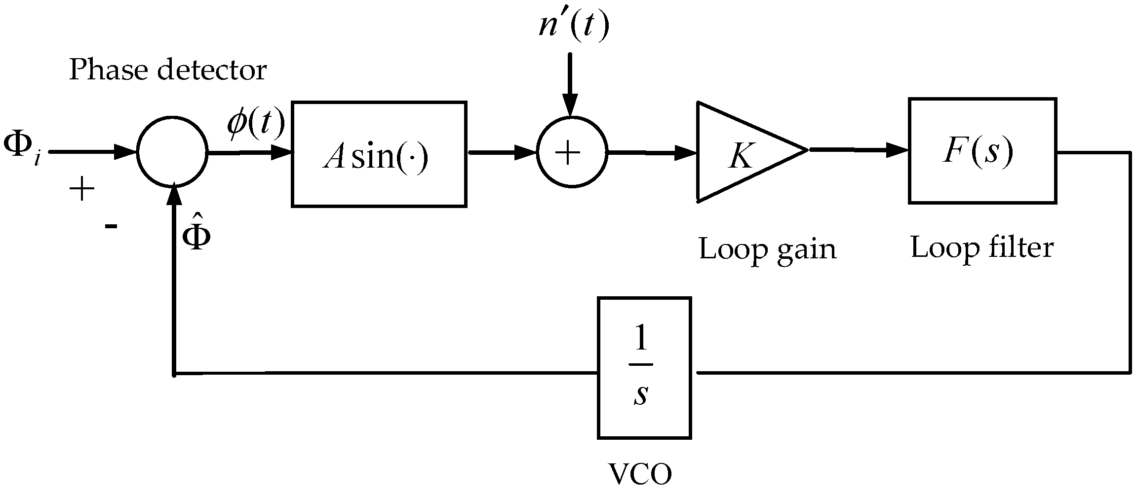
The basic PLL configuration contains a phase detector (PD), for detecting the phase error between the output and the input through feedback system; a loop filter; and a voltage-controlled oscillator (VCO), which is the oscillator to be synchronized by adjusting the phase difference. The mathematical block diagram of the phase-locked loop is shown as in Figure 1. The transfer function $F(s)$ represents the loop filter of a tracking loop. The loop filter is usually a low-pass filter used to suppress the noise and high-frequency signal components from the phase-detector/delay discriminator and provide a dc-controlled signal for the VCO. A first-order tracking loop is obtained when $F(s)=1$.

The equation describing the loop operation is the first-order differential equation given as [1,2,3,4,10,30]

$$\frac{d\varphi (t)}{dt}=(\omega -{\omega }_o)-K[A\sin \varphi (t)+n^{\prime }(t)]$$

(1)

where $\varphi ={\mathsf{\Phi }}_i-\mathsf{\Phi }$ is the error between the phase angle of the incoming signal and the output of the VCO, $K$ is the total loop gain, $A$ is the input signal voltage amplitude, ${\omega }_o$ is the quiescent frequency of the VCO, and $n^{\prime }(t)$ is a stationary white Gaussian noise (WGN) process. Assume that the input signal to the PLL is a pure sinusoid with the average power of $A^2$ Watt, a constant frequency $\omega$ rad/s, and that the signal is corrupted by a stationary white Gaussian noise with a single-sided power spectral density $N_0$ Watt/Hz. For a continuous Markov process, the instantaneous probability density function (PDF) of the phase error $\varphi$ at time $t$, $p(\varphi ,t)$, satisfies the partial differential equation

$$\frac{\partial p(\varphi ,t)}{\partial t}=-\frac{\partial }{\partial \varphi }[A(\varphi )p(\varphi ,t)]+\frac{1}{2}\frac{{\partial }^2}{\partial {\varphi }^2}[B(\varphi )p(\varphi ,t)]$$

(2)

with the initial condition

$$p(\varphi ,0)=\delta (\varphi -{\varphi }_o)$$

(3)

where ${\varphi }_o$ is the initial value of $\varphi$; $A(\varphi )$ and $B(\varphi )$ are normalized moments of the infinitesimal increment [10]. The equation that describes the stochastic behavior of the phase error $\varphi (t)$ of the first order PLL is the Fokker–Planck equation

$$\frac{\partial p(\varphi ,t)}{\partial t}=\frac{\partial }{\partial \varphi }[f(\varphi ,t)p(\varphi ,t)]+\frac{K^2{N}_0}{4}\frac{{\partial }^{2}p(\varphi ,t)}{\partial {\varphi }^2}$$

(4)

where

$$f(\varphi ,t)=AK\sin \varphi (t)+({\omega }_o-\omega )$$

(5)

After substituting Equation (5) into Equation (4), the Fokker–Planck equation that describes the PDF $p(\varphi ,t)$ of the Markov process phase error $\varphi (t)$ can be written as

$$\frac{\partial p(\varphi ,t)}{\partial t}=\frac{\partial }{\partial \varphi }[(AK\sin \varphi +{\omega }_o-\omega )p(\varphi ,t)]+\frac{K^2{N}_0}{4}\frac{{\partial }^{2}p(\varphi ,t)}{\partial {\varphi }^2}$$

(6)

Although the equation is linear in $p$, the complete solution for $p(\varphi ,t)$ is somewhat complicated by the nonlinear behavior of the variable coefficients [10,14].

After normalization, Equation (6) can be expressed as

$$\frac{\partial p(\varphi ,\tau )}{\partial \tau }=\frac{\partial }{\partial \varphi }[(\sin \varphi -\gamma )p(\varphi ,\tau )]+\frac{1}{\alpha }\frac{{\partial }^{2}p(\varphi ,\tau )}{\partial {\varphi }^2}$$

(7)

and alternatively

$$\frac{\partial p(\varphi ,\tau )}{\partial \tau }=(\sin \varphi -\gamma )\frac{\partial p(\varphi ,\tau )}{\partial \varphi }+p\cos \varphi +\frac{1}{\alpha }\frac{{\partial }^{2}p(\varphi ,\tau )}{\partial {\varphi }^2}$$

(8)

if the following variables are employed: loop noise bandwidth $B_L=AK/4$; close-loop signal-to-noise ratio (SNR) $\alpha =A^2/(N_o{B}_L)$; detuning factor $\gamma =(\omega -{\omega }_o)/(4B_L)$; and normalized time $\tau =4B_{L}t$.

2.1. Nonmodulo-2π Phase-Error PDF

An initial distribution of the dependent variable and two sets of boundary conditions are required for a complete description of the problem. Equation (7) can be solved for the PDF of phase error with the initial condition

$$\underset{t\to 0}{\lim }p(\varphi ,t)=\delta (\varphi -{\varphi }_o)$$

(9)

and normalizing condition

$${\displaystyle {\int }_{-\infty }^{\infty }p(\varphi ,\tau )}d\varphi =1$$

(10)

where $\delta (\varphi -{\varphi }_o)$ is the unit impulse function, also known as the Dirac delta function possessing the following property

$$\delta (\varphi -{\varphi }_o)=\{\begin{array}{c}\begin{array}{cc}0,& \varphi \ne {\varphi }_o\end{array}\\ \begin{array}{cc}\infty ,& \varphi ={\varphi }_o\end{array}\end{array};{\displaystyle {\int }_{-\infty }^{\infty }\delta (\varphi -{\varphi }_o)}d\varphi =1$$

(11)

The PDF $p(\varphi ,\tau )$ can be written as

$$p(\varphi ,\tau )=g(\varphi ,\tau )e^{k(\varphi )}$$

(12)

which can be substituted into Equation (7) and lead to the following equation

$$\frac{\partial g(\varphi ,\tau )}{\partial \tau }{e}^{k(\varphi )}=\frac{\partial }{\partial \varphi }[(\sin \varphi -\gamma )g(\varphi ,\tau )e^{k(\varphi )}]+\frac{1}{\alpha }\frac{{\partial }^2[g(\varphi ,\tau )e^{k(\varphi )}]}{\partial {\varphi }^2}$$

(13)

The function $k(\varphi )$ can be found to be [31]

$$k(\varphi )={\displaystyle \int -\alpha (\sin \varphi -\gamma )}d\varphi =\alpha (\cos \varphi +\gamma \varphi )$$

(14)

and consequently, Equation (12) becomes

$$p(\varphi ,\tau )=g(\varphi ,\tau )e^{\alpha (\cos \varphi +\gamma \varphi )}$$

(15)

where the density function $g(\varphi ,\tau )$ satisfies the following one-dimensional advection–diffusion parabolic PDE, called the modified FP equation

$$\frac{\partial g(\varphi ,\tau )}{\partial \tau }=(\gamma -\sin \varphi )\frac{\partial g(\varphi ,\tau )}{\partial \varphi }+\frac{1}{\alpha }\frac{{\partial }^{2}g(\varphi ,\tau )}{\partial {\varphi }^2}$$

(16)

Solving for $g(\varphi ,\tau )$ is computationally simpler than solving for $p(\varphi ,\tau )$, mainly due to the fact that coarser grid spacing is allowed for $g(\varphi ,\tau )$. Additionally, $p(\varphi ,\tau )$ can be reconstructed readily using Equation (15) without difficulty when $g(\varphi ,\tau )$ is obtained.

2.2. Modulo-2π Phase-Error PDF

A common form of partial solution to Equation (7) is the modulo-2π probability [1,2,3,4,10,11,12,13]

$$P(\varphi ,\tau )={\displaystyle \sum _{k=-\infty }^{\infty }p(\varphi +k2\pi ,\tau )}$$

(17)

where the capital letter $\mathrm{P}$ is used to denote the modulo-2π PDF while little letter $p$ denotes the unbounded nonmodulo-2π PDF, respectively. In the steady state, $p(\varphi ,\tau )$ is spread over all $\varphi$ since cyclic slipping event (lock on at $k2\pi$) have occurred. The relation between these two PDF’s can be expressed as

$$P(-\pi <\varphi <\pi ,\tau )=p(\varphi ,\tau )\mathrm{modulo}2\pi$$

(18)

which shows that $P(\varphi ,\tau )$ has a period of 2π rad. This is like the original function except that each 2π-wide region contains an identical distribution and $\mathrm{P}$ begins with impulses at $k2\pi$ for all $k$. As $\mathrm{P}$ diffuses with time, the probability that the phase will jump out of the primary interval $-\pi <\varphi <\pi$ is the same as the probability that it will jump into that interval. As time increases, $p(\varphi ,\tau )$ diffuses so the ultimate value approaches zero everywhere. Consider only the interval $-\pi <\varphi <\pi$ and set the boundary and normalized conditions, respectively:

$$P(\pi ,\tau )=P(-\pi ,\tau );{\displaystyle {\int }_{-\pi }^{\pi }P(\varphi ,\tau )}d\varphi =1$$

(19)

Hence the modulo-2π PDF describing the phase error is obtained.

2.3. Cyclic Slipping Density Function

A cycle slip is defined as an increase (positive cycle slip) or decrease (negative cycle slip) of the phase error by 2π. Cycle slipping in a phase-locked oscillator occurs where the dynamic phase error is larger than 2π. If the error should become too large that the VCO skips cycles, the loop is considered to have lost lock. The integral of this density becomes

$${\displaystyle {\int }_{-2\pi }^{2\pi }q(\varphi ,\tau )}d\varphi \to 0\mathrm{as}\tau \to \infty$$

(20)

As long as the loop phase error remains within the limits of a specified subinterval, the density function $q(\varphi ,\tau )$, accompanied with the initial condition $q(\varphi ,0)=\delta (\varphi )$, will satisfy the FP equation

$$\frac{\partial q(\varphi ,\tau )}{\partial \tau }=\frac{\partial }{\partial \phi }[(\sin \varphi -\gamma )q(\varphi ,\tau )]+\frac{1}{\alpha }\frac{{\partial }^{2}q(\varphi ,\tau )}{\partial {\varphi }^2}$$

(21)

and thus

$$\frac{\partial q(\varphi ,\tau )}{\partial \tau }=(\sin \varphi -\gamma )\frac{\partial q(\varphi ,\tau )}{\partial \varphi }+q(\varphi ,\tau )\cos \varphi +\frac{1}{\alpha }\frac{{\partial }^{2}q(\varphi ,\tau )}{\partial {\varphi }^2}$$

(22)

The use of $q(\varphi ,\tau )$ for the bounded case is to distinguish it from the unbounded nonmodulo-2π function $p(\varphi ,\tau )$. The numerical algorithm used to generate $q(\varphi ,\tau )$ is the same as for generating $p(\varphi ,\tau )$, except that the end points $q({\varphi }_l,\tau )$ and $q(-{\varphi }_l,\tau )$ are forced to be zero, whereas the end points for $p(\varphi ,\tau )$ were found by extrapolation, which simulates an infinite interval.

3. Numerical Formulations for the Normalized Fokker–Planck Equation

The solution procedure of a PDE depends on the type of the equation. Imposition of initial and/or boundary conditions also depends on the type of PDE. To make this paper self-contained, the main steps for discretization of the typical model equations are introduced first. After that, numerical formulations using the implicit method for the normalized Fokker–Planck equation are presented.

3.1. Discretization of the Model Equation

The heat conduction equation is a parabolic PDE with the form

$$\frac{\partial u}{\partial t}=\rho \frac{{\partial }^{2}u}{\partial x^2}$$

(23)

which is typically characterized by a diffusivity (or dispersion) coefficient $\rho$. The convective (or advection) equation such as the wave equation is categorized as a hyperbolic type given by

$$\frac{\partial u}{\partial t}+v\frac{\partial u}{\partial x}=0$$

(24)

Consider the one-dimensional transport equation with both convection and diffusion terms,

$$\frac{\partial u}{\partial t}=-v\frac{\partial u}{\partial x}+\rho \frac{{\partial }^{2}u}{\partial x^2},\mathrm{where}v=\mathrm{const},\rho =\mathrm{const}>0$$

(25)

where $u$ is a scalar, being convected with a known velocity $v$ and being diffused. Equation (25) is a one-dimensional non-linear convective diffusion equation, or a hyperbolic parabolic equation; it is hyperbolic due to the convective term, $v\partial u/\partial x$, and it is parabolic due to the diffusive term, $\rho {\partial }^{2}u/\partial x^2$. Like the diffusion equation the transport equation is strictly parabolic. Closed-form solution $u(x,t)$ of Equation (25) is usually not available except for very simplified cases. It can, however, be obtained numerically in most applications, for example, by the finite difference and the finite element methods. The transport equation, as the model equation in this paper, will be implemented.

Explicit methods are easier to solve than implicit methods in terms of time and effort spent on a computer. However, there exist several disadvantages in explicit methods. For the explicit finite difference method to be stable, the grid spacing in the time domain and grid spacing in the space domain need to satisfy certain requirements. The choice of grid spacing is made in accordance with the condition of stability. Implicit methods offer great advantage on the stability of the finite difference equations, since most are unconditionally stable. Therefore, a larger grid size in time is permitted. It should be noted that the selection of a larger time step is limited due to accuracy consideration because an increase in time step will increase the truncation error of the finite difference equation.

In the finite-difference methods, partial derivatives are approximated using Taylor’s series; hence, solutions can be obtained using the first-, second-, or higher-order accurate methods. In this paper, the following finite difference approximations are selected for the partial derivatives:

$$\frac{\partial u(x,t)}{\partial t}=\frac{u(x,t+\Delta t)-u(x,t)}{\Delta t}+O(\Delta t)\approx \frac{u_j^{n+1}-u_j^n}{\Delta t}$$

(26)

$$\frac{\partial u(x,t)}{\partial x}=\frac{u(x+\Delta x,t)-u(x-\Delta x,t)}{2\Delta x}+O{(\Delta x)}^2\approx \frac{u_{j+1}^{n+1}-u_{j-1}^{n+1}}{2\Delta x}$$

(27)

$$\frac{{\partial }^{2}u(x,t)}{\partial x^2}=\frac{u(x+\Delta x,t)-2u(x,t)+u(x-\Delta x,t)}{{(\Delta x)}^2}+O{(\Delta x)}^2\approx \frac{u_{j+1}^{n+1}-2u_j^{n+1}+u_{j-1}^{n+1}}{{(\Delta x)}^2}$$

(28)

An equation is defined as being implicit when more than one unknown appears in the finite difference equation. For the implicit methods, a set of simultaneous equations needs to be solved, which requires more computation time per time step for the implicit methods. Implicit methods generally possess better stability properties and higher accuracy than the explicit methods. For implicit formulation, most are unconditionally stable. Implicit methods include (1) the backward time/central space (BTCS) implicit method, and (2) the Crank–Nicolson (CN) method. For the model equation, the BTCS implicit scheme, also known as the simple (Laasonen) implicit scheme, leads to the following formulation

$$\frac{u_j^{n+1}-u_j^n}{\Delta t}=-\nu \frac{u_{j+1}^{n+1}-u_{j-1}^{n+1}}{2\Delta x}+\rho \frac{u_{j+1}^{n+1}-2u_j^{n+1}+u_{j-1}^{n+1}}{{(\Delta x)}^2}$$

(29)

or

$$u_j^{n+1}+\frac{c}{2}(u_{j+1}^{n+1}-u_{j-1}^{n+1})-d(u_{j+1}^{n+1}-2u_j^{n+1}+u_{j-1}^{n+1})=u_j^n$$

(30)

which can be rearranged as

$$-(d+\frac{c}{2})u_{j-1}^{n+1}+(1+2d)u_j^{n+1}-(d-\frac{c}{2})u_{j+1}^{n+1}=u_j^n$$

(31)

By considering all spatial nodes Equation (31) produces a tridiagonal system of equations that can be solved efficiently using the Thomas algorithm [17].

The CN scheme evaluates the spatial derivative at the average of the $n$th and $(n+1)$-th time levels, i.e., at the $(n+1/2)$-th time level. For the model equation, the CN scheme gives

$$\frac{u_j^{n+1}-u_j^n}{\Delta t}=-0.5v\left(\frac{u_{j+1}^n-u_{j-1}^n}{2\Delta x}+\frac{u_{j+1}^{n+1}-u_{j-1}^{n+1}}{2\Delta x}\right)+0.5\rho \left(\frac{u_{j-1}^n-2u_j^n+u_{j+1}^n}{{(\Delta x)}^2}+\frac{u_{j-1}^{n+1}-2u_j^{n+1}+u_{j+1}^{n+1}}{{(\Delta x)}^2}\right)$$

(32)

which can be rewritten as

$$-(d+\frac{c}{2})u_{j-1}^{n+1}+2(1+d)u_j^{n+1}-(d-\frac{c}{2})u_{j+1}^{n+1}=(d+\frac{c}{2})u_{j-1}^n+2(1-d)u_j^n+(d-\frac{c}{2})u_{j+1}^n$$

(33)

Equation (33) is consistent with Equation (25) with a truncation error of $O[{(\Delta t)}^2,{(\Delta x)}^2]$ since the Taylor expression is made about $(j,n+1/2)$, hence second-order accurate spatial differences are inserted into this algorithm. The CN method offers a considerable improvement over the FTCS and BTCS implicit schemes whose local truncation errors are only first-order accurate in time. A von Neumann stability analysis indicates that the CN scheme is unconditionally stable.

3.2. Discretization of the Normalized Fokker–Planck Equation

The modified FP equation is a one-dimensional non-linear hyperbolic parabolic PDE in which both convection and diffusion terms are involved. The numerical algorithms for the FP equation can be obtained based on the procedures discussed in Section 3.1. The equation to be solved is Equation (16), which is analogous to the model equation, Equation (25), with the relations:

$$\nu =\sin \phi -\gamma ;\rho =\frac{1}{\alpha }$$

(34)

The implicit finite difference methods are computationally advantageous methods with respect to the explicit ones since they are unconditionally stable. In addition to the Euler’s BTCS implicit method, the CN method is second-order accurate both in time and space domains.

Applying the Euler’s BTCS implicit scheme for the FP equation, we have the following formulation for numerical implementation

$$\frac{g_j^{n+1}-g_j^n}{\Delta \tau }=(\gamma -\sin \varphi )\frac{g_{j+1}^{n+1}-g_{j-1}^{n+1}}{2\Delta \varphi }+\frac{1}{\alpha }\frac{g_{j+1}^{n+1}-2g_j^{n+1}+g_{j-1}^{n+1}}{{(\Delta \varphi )}^2}$$

(35)

and

$$g_j^{n+1}-g_j^n=(\gamma -\sin \varphi )\frac{\Delta \tau }{2\Delta \varphi }(g_{j+1}^{n+1}-g_{j-1}^{n+1})+\frac{\Delta \tau }{\alpha {\left(\Delta \varphi \right)}^2}(g_{j+1}^{n+1}-2g_j^{n+1}+g_{j-1}^{n+1})$$

(36)

which can be rearranged

$$\left[\left(\gamma -\sin \varphi \right)\frac{\Delta \tau }{2\Delta \varphi }-\frac{\Delta \tau }{\alpha {\left(\Delta \varphi \right)}^2}\right]g_{j-1}^{n+1}+\left[1+\frac{2\Delta \tau }{\alpha {(\Delta \varphi )}^2}\right]g_j^{n+1}-\left[\left(\gamma -\sin \varphi \right)\frac{\Delta \tau }{2\Delta \varphi }+\frac{\Delta \tau }{\alpha {(\Delta \varphi )}^2}\right]g_{j+1}^{n+1}=g_j^n$$

(37)

Equation (37) can be represented as

$$-(\eta +\frac{\xi }{2})g_{j-1}^{n+1}+(1+2\eta )g_j^{n+1}-(\eta -\frac{\xi }{2})g_{j+1}^{n+1}=g_j^n$$

(38)

where $\xi =\left(\sin \phi -\gamma \right)\frac{\Delta \tau }{\Delta \phi }$, representing the Courant number, and $\eta =\frac{\Delta \tau }{\alpha {(\Delta \varphi )}^2}$, representing the diffusion number.

Employing the CN scheme, we have

$$\frac{g_j^{n+1}-g_j^n}{\Delta \tau }=\left(\gamma -\sin \varphi \right)\frac{{\overline{\delta }}_{\varphi }{g}_j^n+{\overline{\delta }}_{\varphi }{g}_j^{n+1}}{4\Delta \varphi }+\frac{1}{\alpha }\frac{{\delta }_{\varphi }^2{g}_j^n+{\delta }_{\varphi }^2{g}_j^{n+1}}{2{(\Delta \varphi )}^2}$$

(39)

With the finite-difference operators defined as

$${\overline{\delta }}_{\varphi }{g}_j^n=g_{j+1}^n-g_{j-1}^n;{\delta }_{\varphi }^2{g}_j^n=g_{j+1}^n-2g_j^n+g_{j-1}^n$$

(40)

the CN implicit formulation, after rearrangement, is given by

$$-(\eta +\frac{\xi }{2})g_{j-1}^{n+1}+2(1+\eta )g_j^{n+1}-(\eta -\frac{\xi }{2})g_{j+1}^{n+1}=(\eta +\frac{\xi }{2})g_{j-1}^n+2(1-\eta )g_j^n+(\eta -\frac{\xi }{2})g_{j+1}^n$$

(41)

4. Numerical Implementation and Analysis of the Phase-Locked Loop Statistics

In this section, numerical implementation and analysis of the first-order phase-locked loop statistics are presented by solving the normalized FP equation. Computer codes were developed using the Matlab^® software. According to Equation (9), the initial condition is supposed to be a Dirac delta function. Since the delta function is a continuous-time signal and therefore, for numerically resolved purpose, the value $1/\Delta \varphi$ is used for approximating the delta function. In the following illustrative examples, the initial value of phase error ${\varphi }_0=0$ is utilized for discussion.

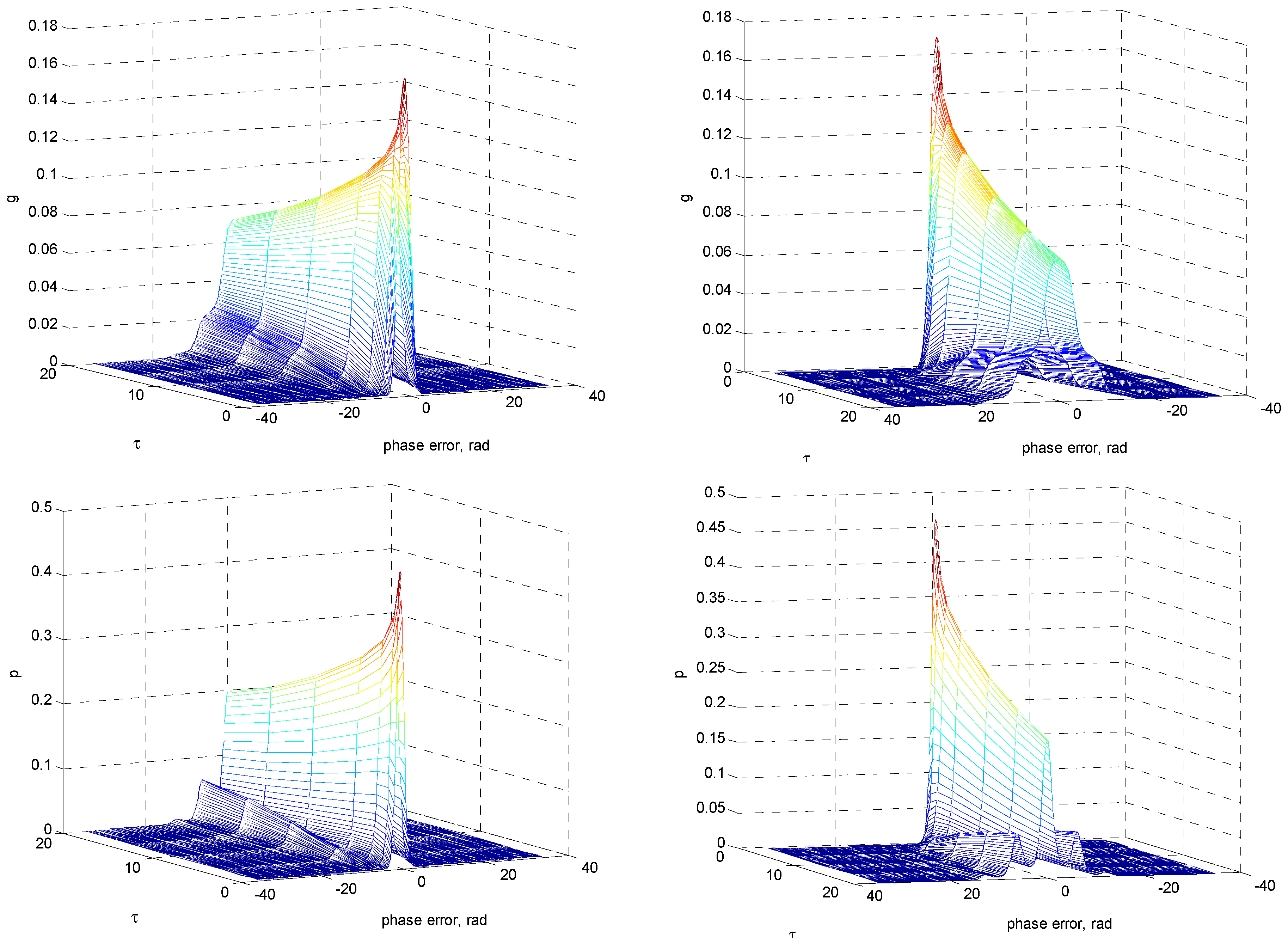
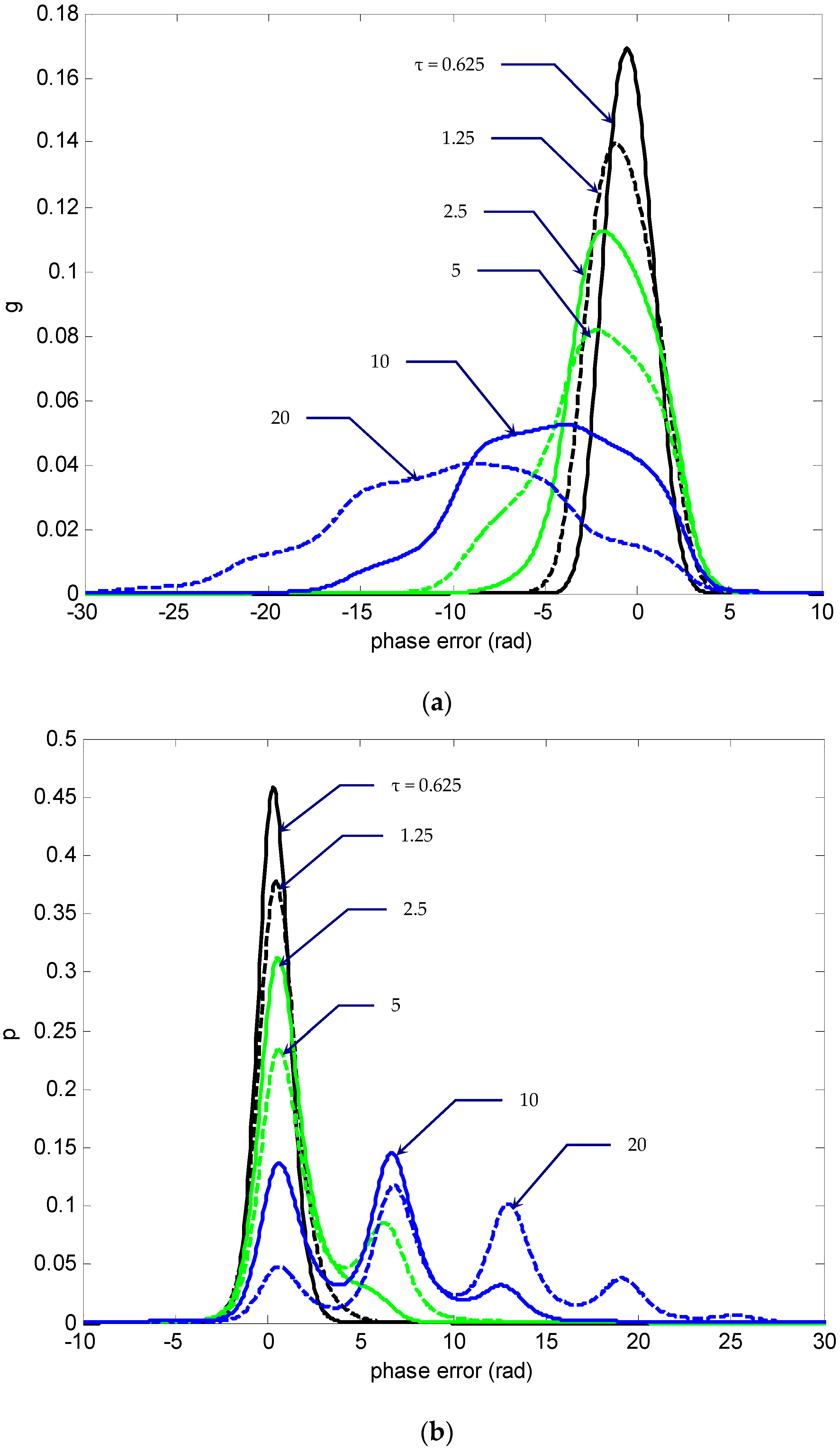
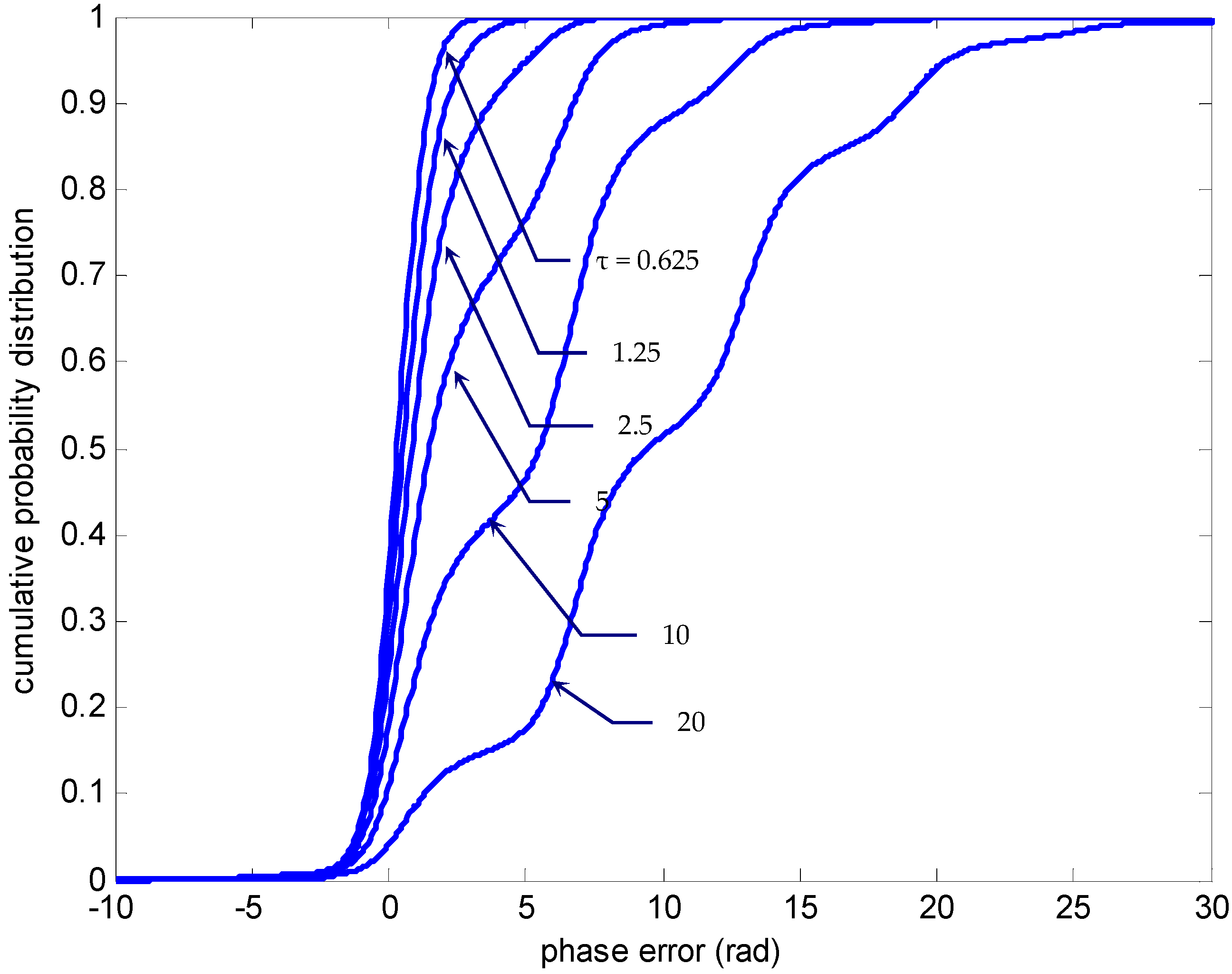
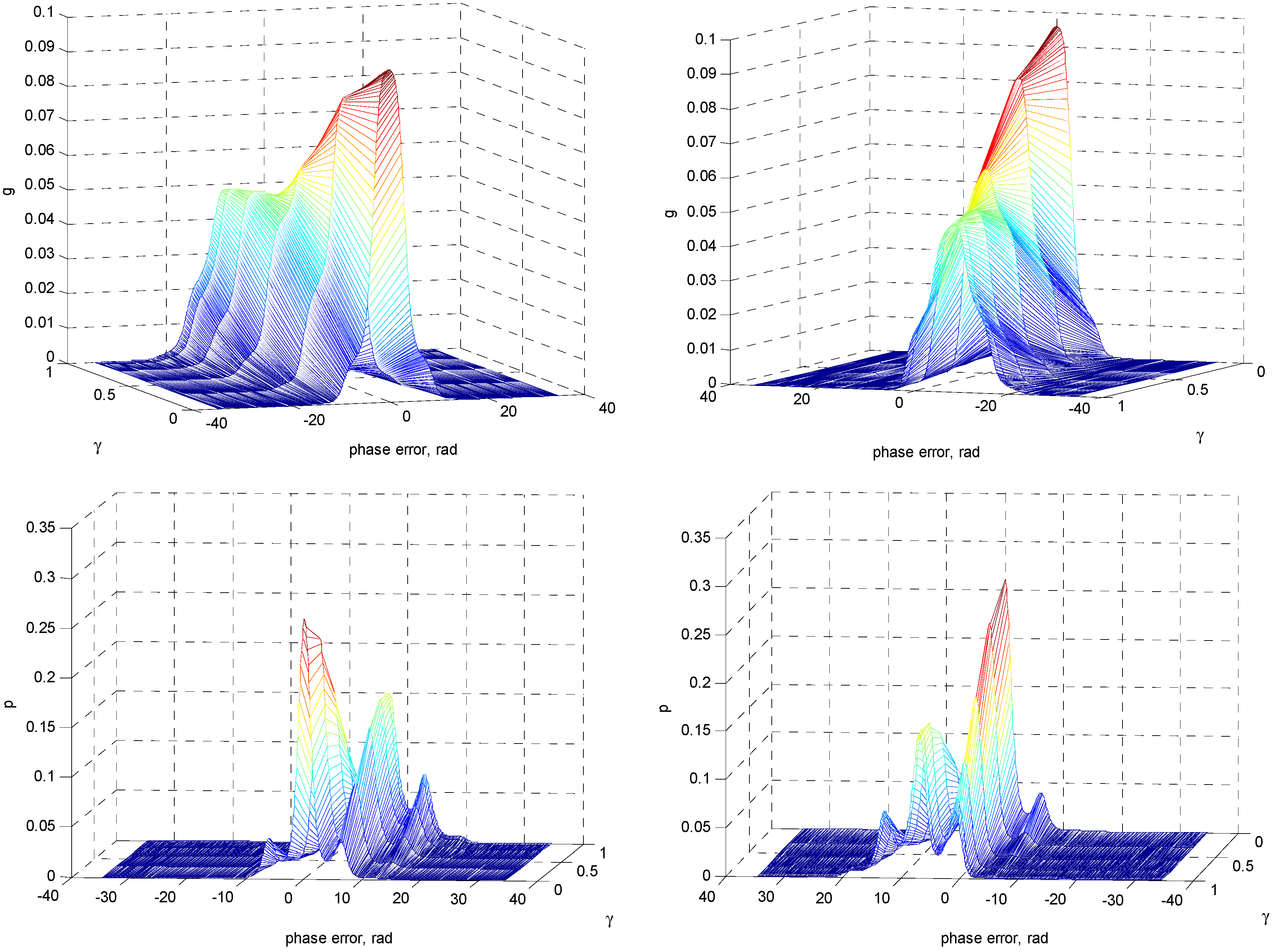
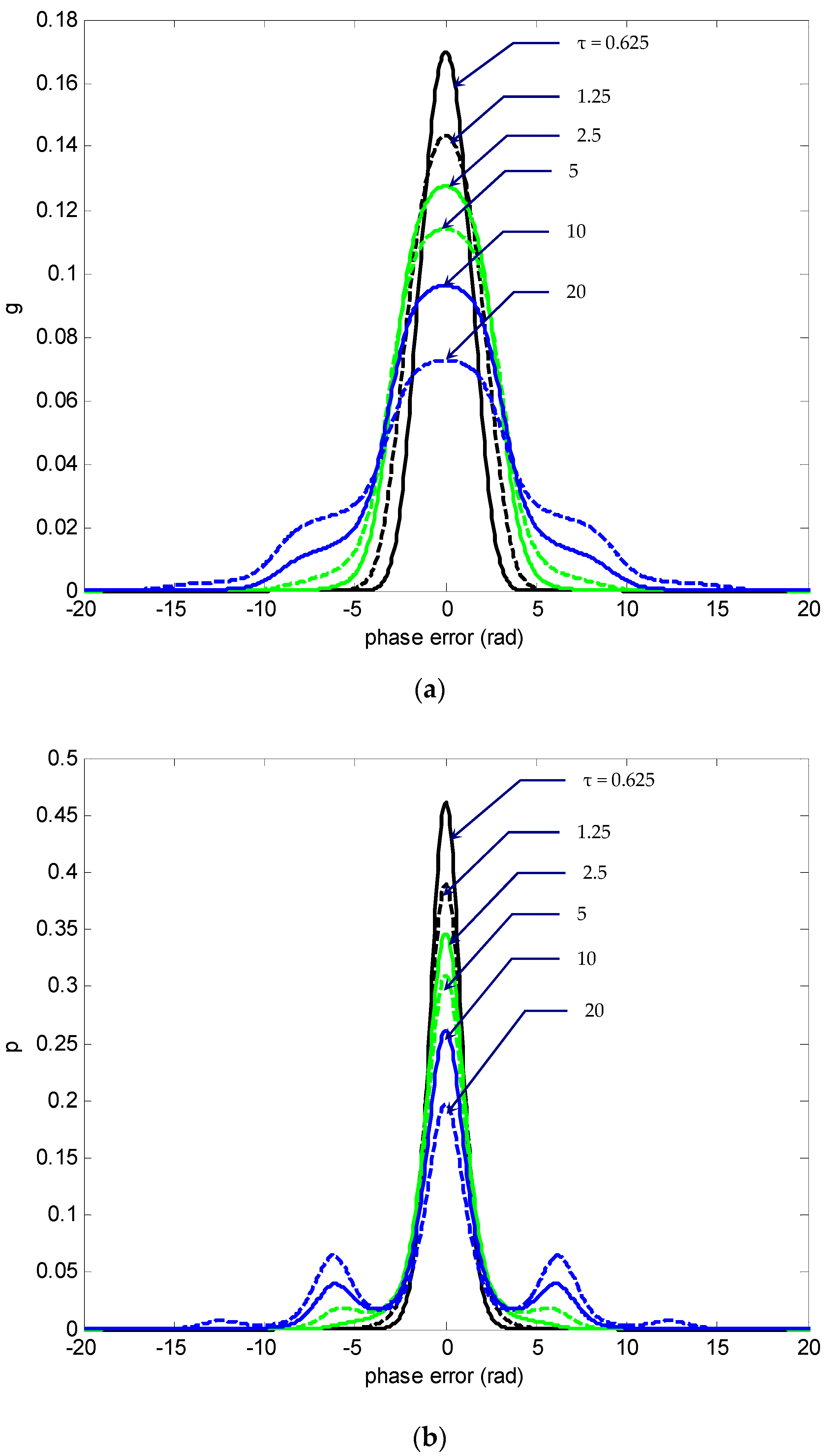
First of all, the time-evolution of PDFs is investigated to reveal detailed evolution of the time-dependent PDFs of the PLL. Typical results for the time-evolution of nonmodulo-2π transient statistics for SNR $\alpha =1$ and detuning factor $\gamma =0$ are shown in Figure 2, Figure 3 and Figure 4. The grid spacing for the phase-error domain is chosen as $\Delta \varphi =\pi /50$ rad; the grid spacing in the time marching direction is set as 0.01. Figure 2 shows the transition phase-error density function $g(\varphi ,\tau )$ and the PDF $p(\varphi ,\tau )$. The numbers beside individual curves indicate the normalized times, switching τ from 0.625 to 20. The corresponding cumulative probability distribution of the phase-error is depicted in Figure 3. Typical time-evolution of $p(\varphi ,\tau )$, as shown in Figure 2b, revealed that as P diffused with time, the probability that the phase would jump out of the primary interval $-\pi <\varphi <\pi$ was the same as the probability that it would jump into that interval, implying that the possibility of larger phase error increased. In the case of $\gamma =0$, both of the error density functions $g(\varphi ,\tau )$ and $p(\varphi ,\tau )$ diffuse with time while remaining symmetric with respect to the phase-error axis, and thus the initial global peak values of the density functions g and p at zero phase error ($\varphi =0$) decreased as time progresses. As functions of $\varphi$, the local peak positions of p appeared at a period of 2π rad. The amplitudes of local peaks were monotonically nonincreasing when moving outwards from their mean values with respect to the phase-error axis. The figures and later ones as well only show part of the results. In Figure 2 and Figure 3, the results at a phase error between −20 and 20 rad were the area of interest. Figure 4 provides the three-dimensional plots for nonmodulo-2π transition g and p, respectively, for more profound insights into the statistics information, especially the relation between g/p and phase error, as time progresses. Both the front view and back view are shown such that better understanding on the behavior of PLL statistics is accessible. The result enabled us to mathematically quantify the difference among different PDFs, providing a meaningful conceptual link between the stochastic process and information geometry, and could be utilized for optimizing various desired outcomes.

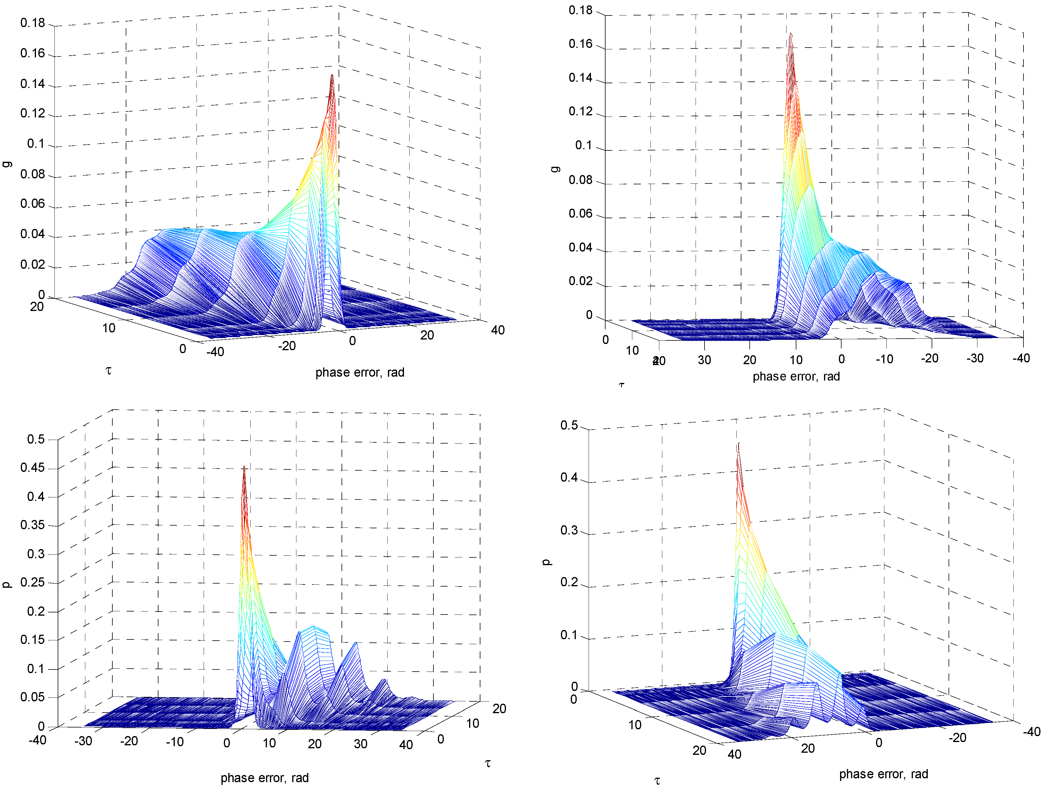
Figure 5, Figure 6 and Figure 7 provide information basically similar to that of Figure 2, Figure 3 and Figure 4, and thus the parameter values were identical except that the detuning factor was now changed to $\gamma =\sin (\pi /4)$. The identical numerical values including the normalized time (τ), the grid size for the phase-error domain ($\Delta \varphi$) and the grid size in the time marching direction ($\Delta \tau$) were utilized for comparison. It can be seen that in this case the density functions diffused to one direction as time progresses, given a certain SNR (e.g.,$\alpha =1$ as demonstrated here). The error probabilities g and p diffused virtually in opposite directions. In this example, g virtually diffused leftwards while p diffused rightwards. As can be seen, p had a right-skewed (or positively skewed) distribution, and most data fell to the right (positive direction) of the graph’s peak. The histogram skewed in such a way that its right side (or “tail”) was longer than its left side. Again, for the density function p, there were local peaks appearing with a period of 2π rad. It should be noticed that the position of global peak of p, which initially appeared at the phase error near by zero, moved rightwards as time progressed. As can be seen, the peak position appeared at 2π rad away from its original position when τ exceeded a certain value, e.g., τ = 10 in this illustration. According to Equation (10), if the solution is properly resolved, the total probability remains constant (=1) for all time. The cumulative probability distribution can be used to check the result. As compared to the actual total probability, the numerically calculated cumulative probabilities for various normalized time are summarized in

Table 1. The numerically calculated cumulative probabilities at various normalized time, for $\gamma =0$ and $\gamma =\sin (\pi /4)$.

Normalized Time (τ)	Cumulative Probabilities
	$\mathit{\gamma }=0$	$\mathit{\gamma }=\mathbf{sin}(\mathit{\pi }/4)$
0.625	0.9998	0.9999
1.25	0.9997	0.9999
2.5	0.9997	0.9996
5	0.9997	0.9990
10	0.9997	0.9978
20	0.9997	0.9954

. The errors using the numerical approach was of the order of 0.02% to 0.5% depending on the various τ, for $\gamma =0$ and $\gamma =\sin (\pi /4)$, respectively. For better resolution that is required, a smaller grid can be utilized.

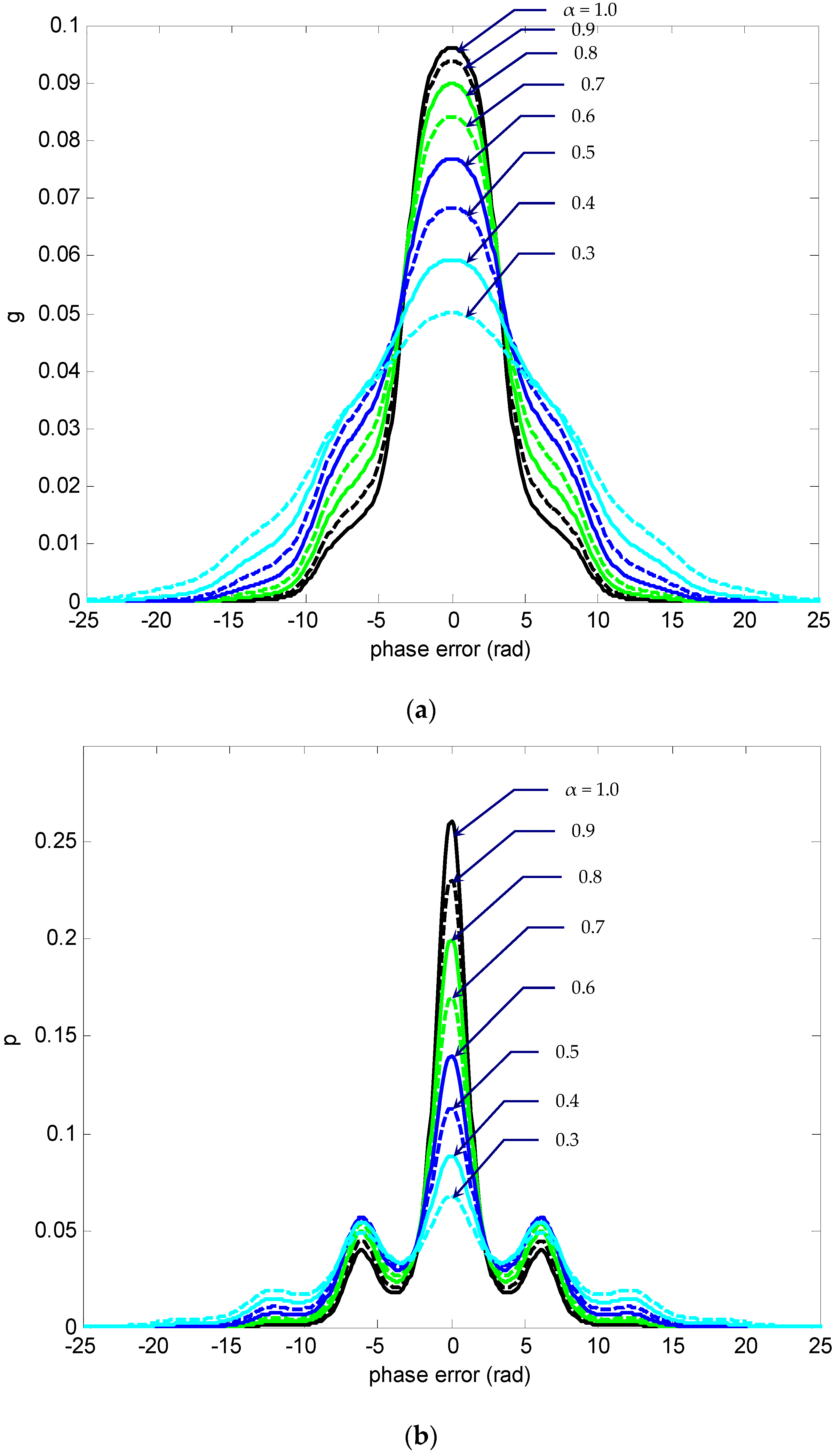
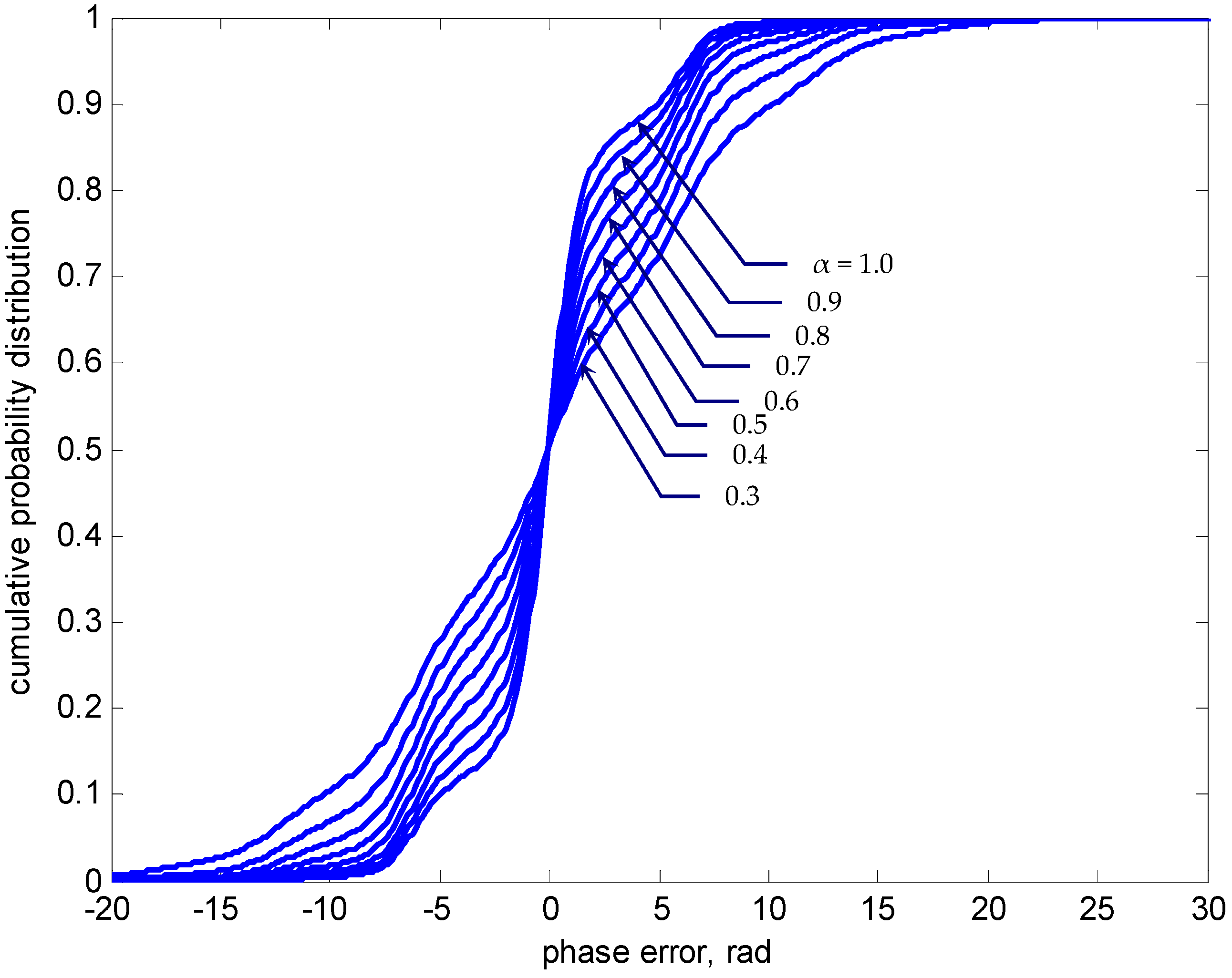
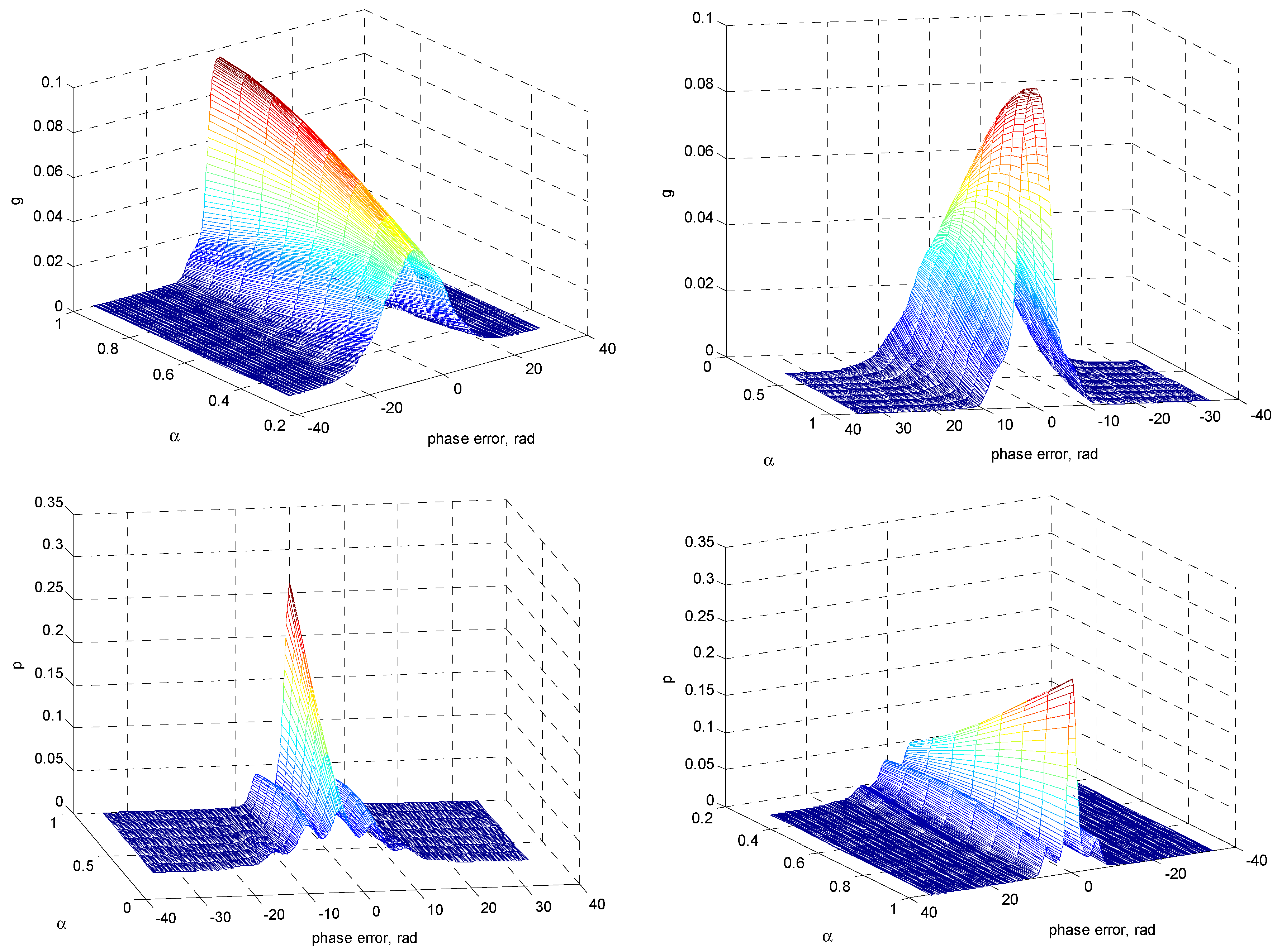
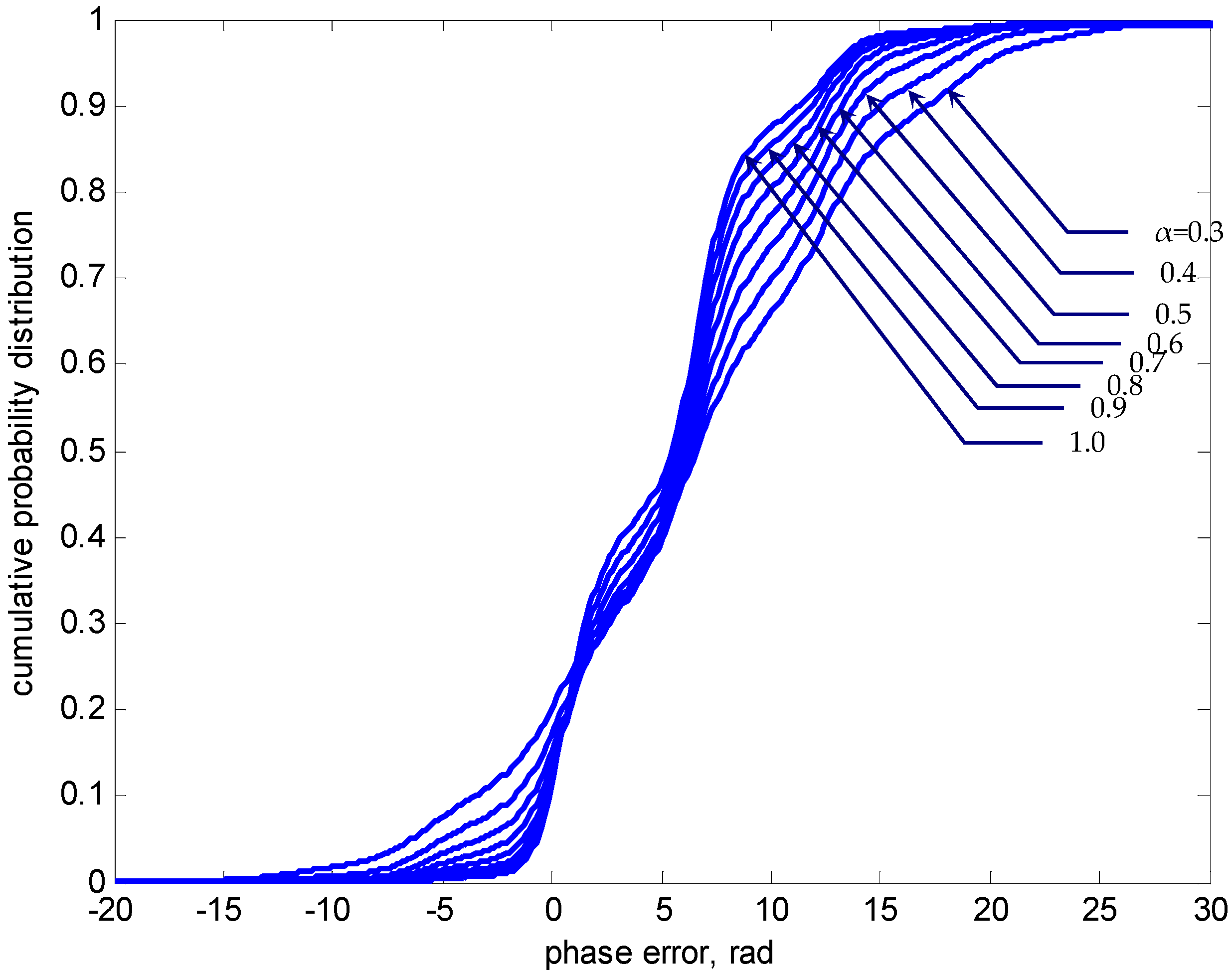
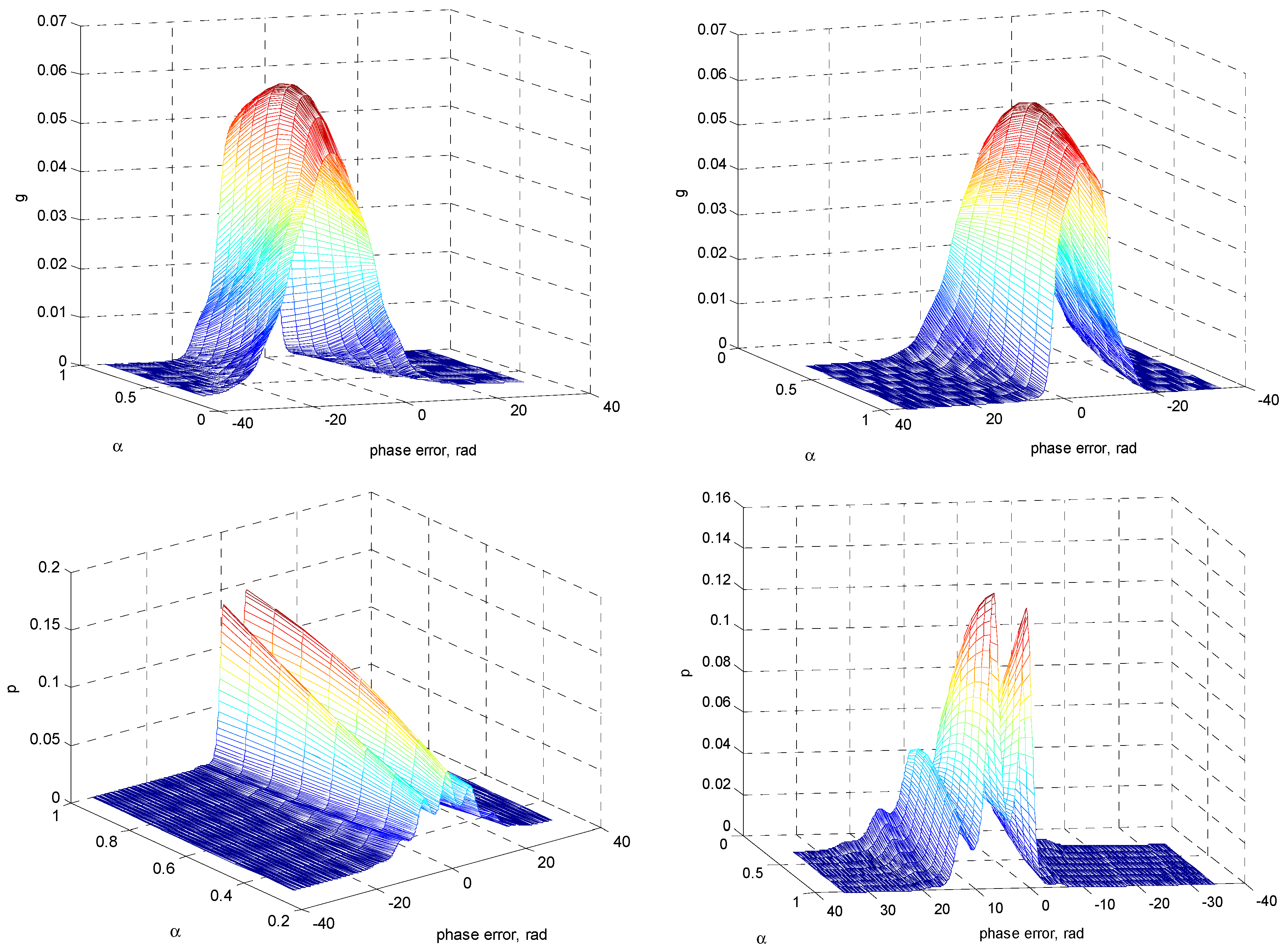
In the next example, an illustration of how the SNR α influences the information geometry of the phase-error statistics is presented. Figure 8, Figure 9 and Figure 10 provide the results of the nonmodulo-2π statistics at normalized time $\tau =10$ for SNR α in the range 0.3–1 where the detuning factor $\gamma =0$ was utilized. The results are shown to capture the effect of different SNR values and understand the information changes on the error-phase statistics of PLL. Figure 8 presents the phase-error density function $g(\varphi ,\tau )$ and the PDF $p(\varphi ,\tau )$ and Figure 9 shows the corresponding cumulative probability distribution of $p(\varphi ,\tau )$. The numbers beside individual curves indicate the various SNR values. Again, three-dimensional plots for nonmodulo-2π g and p, respectively, are given in Figure 10. As in the presented case where $\gamma =0$ was utilized, both the density functions g and p remained symmetric with respect to the phase-error axis as α varied. As α decreased, the global peak values of the density functions at $\varphi =0$ decreased and thus the initial narrow density functions became ‘flatter’, implying that the variance the phase error increased, and the possibility of a larger phase error increased. As functions of $\varphi$, the local peak positions appeared at a period of 2π rad when moving outwards, with the peak amplitudes monotonically nonincreasing.

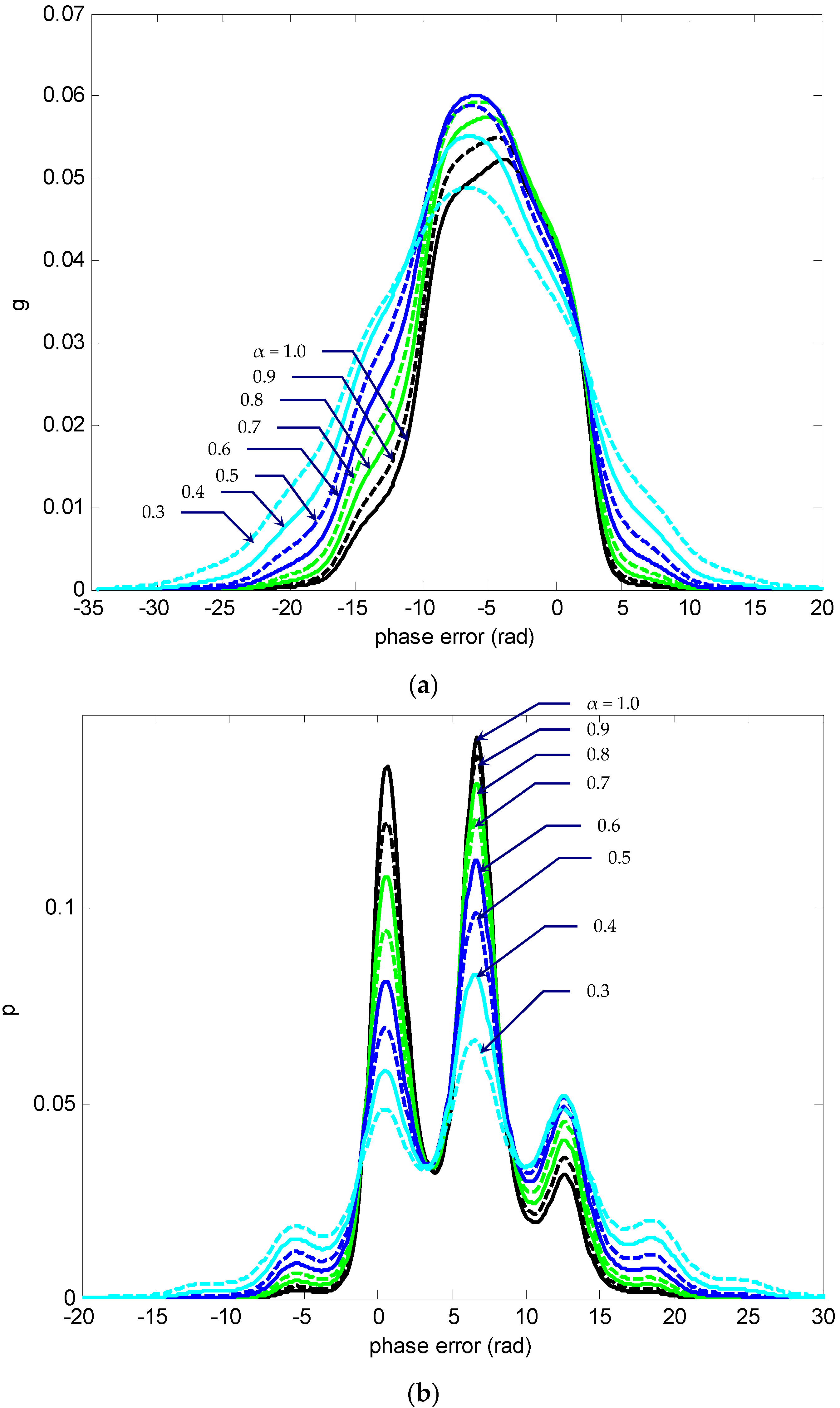
Figure 11, Figure 12 and Figure 13 elucidated information similar to that of Figure 8, Figure 9 and Figure 10, and the parameter values were identical except that the detuning factor $\gamma =\sin (\pi /4)$ was utilized. It can be seen that the density functions g and p virtually stretched (or expanded) to one direction where they stretched to opposite directions. As shown in this example, g had a left-skewed distribution, while p had a right-skewed distribution. The density p shows that the peak values appeared at the phase error near by 2π rad. As α decreased, p tended to be flatter, and the variance of the phase error increased. Three-dimensional plots of information geometry were provided such that more comprehensive understanding could be gained on the relationship among the parameters, p/q, $\varphi$, and α.

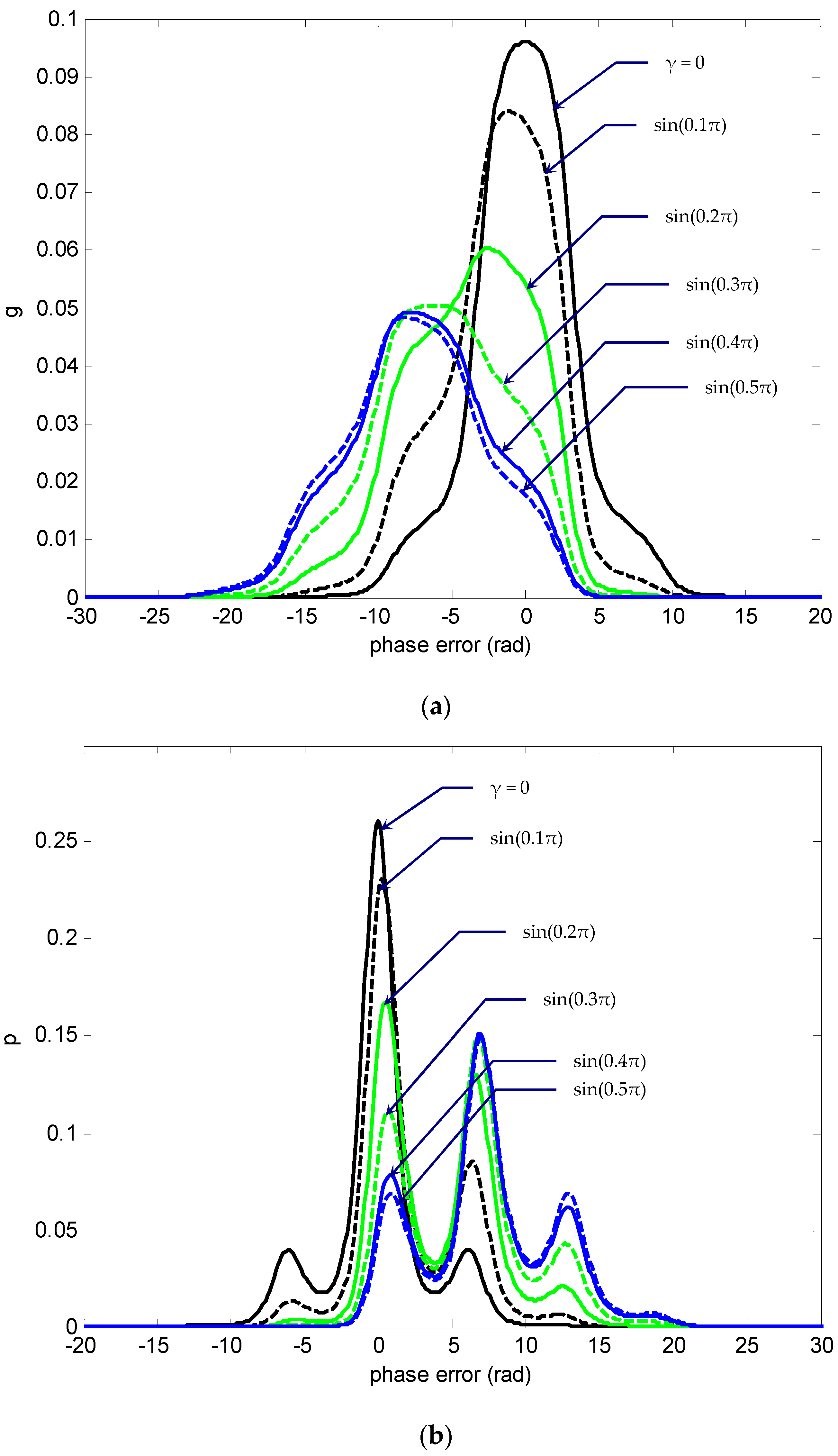
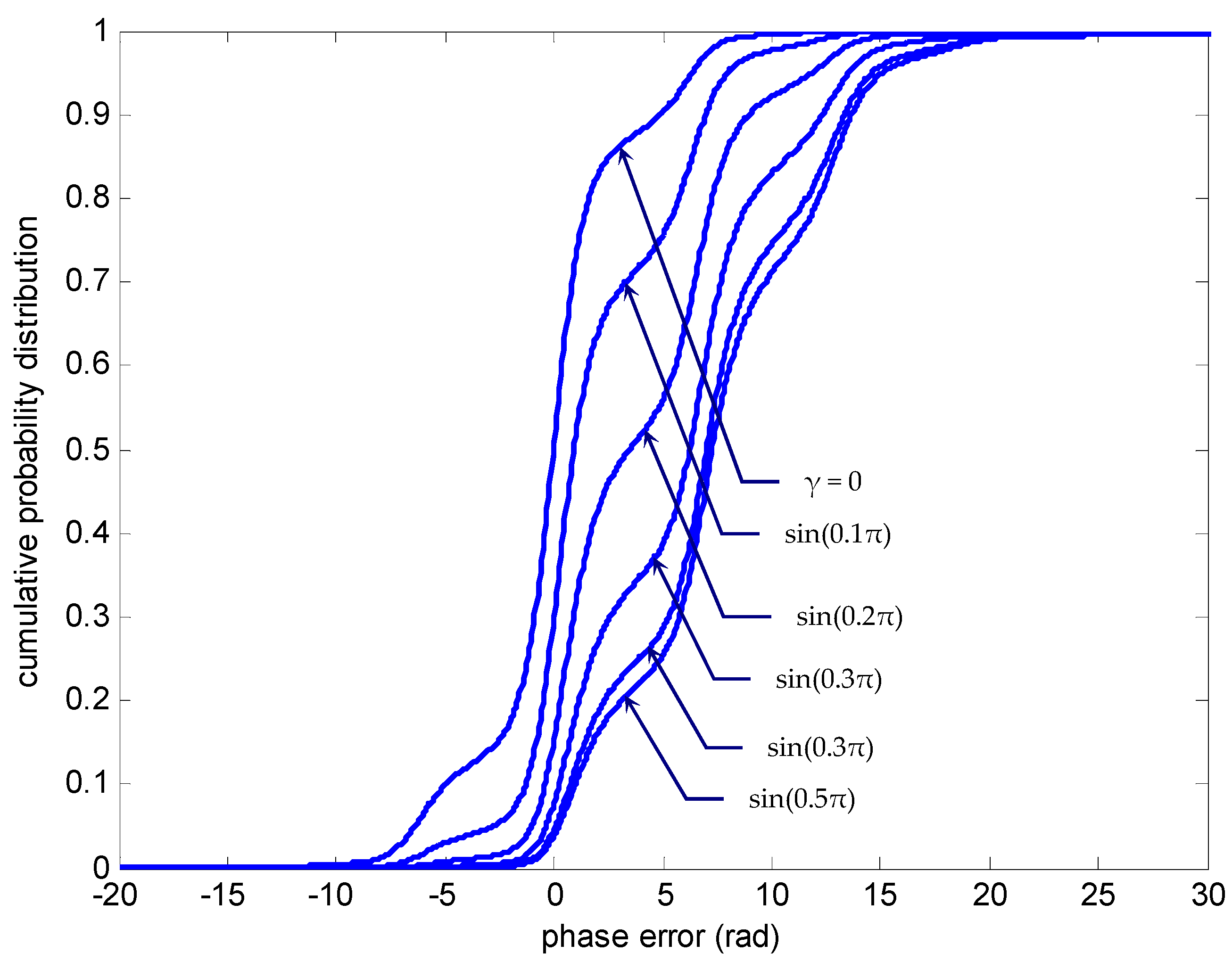
To elucidate the effect of detuning factor $\gamma$ on the error-phase statistics of PLL, the following illustrations are shown. Figure 14, Figure 15 and Figure 16 provide the results for the nonmodulo-2π statistics at normalized time $\tau =10$ for various detuning factors $\gamma$, where the signal was assumed to be sufficient and a high SNR value $\alpha =1$ was utilized for illustration. The numbers beside individual curves indicate the detuning factor $\gamma$, from $\gamma =0$ to $\sin (0.5\pi )$. The density functions stretched to one direction as the detuning factor $\gamma$ increased, where g and p stretched to opposite directions. As can be seen in this example, g moved leftwards while p went rightwards. Furthermore, the increase of the $\gamma$ value caused the density functions to flatten, revealing the possibility of the larger phase error increasing. The global peak of the density function p, which initially appeared at the phase error near by zero, moved rightwards with the increase of $\gamma$. As can be seen from the graphs, the peak position appeared at 2π rad away from its original position when $\gamma$ was sufficiently large, e.g., $\sin (0.3\pi )$ in this example. The three-dimensional plots provided elucidated more comprehensive geometry information on the relationship among the parameters, p/q, $\varphi$, and $\gamma$.

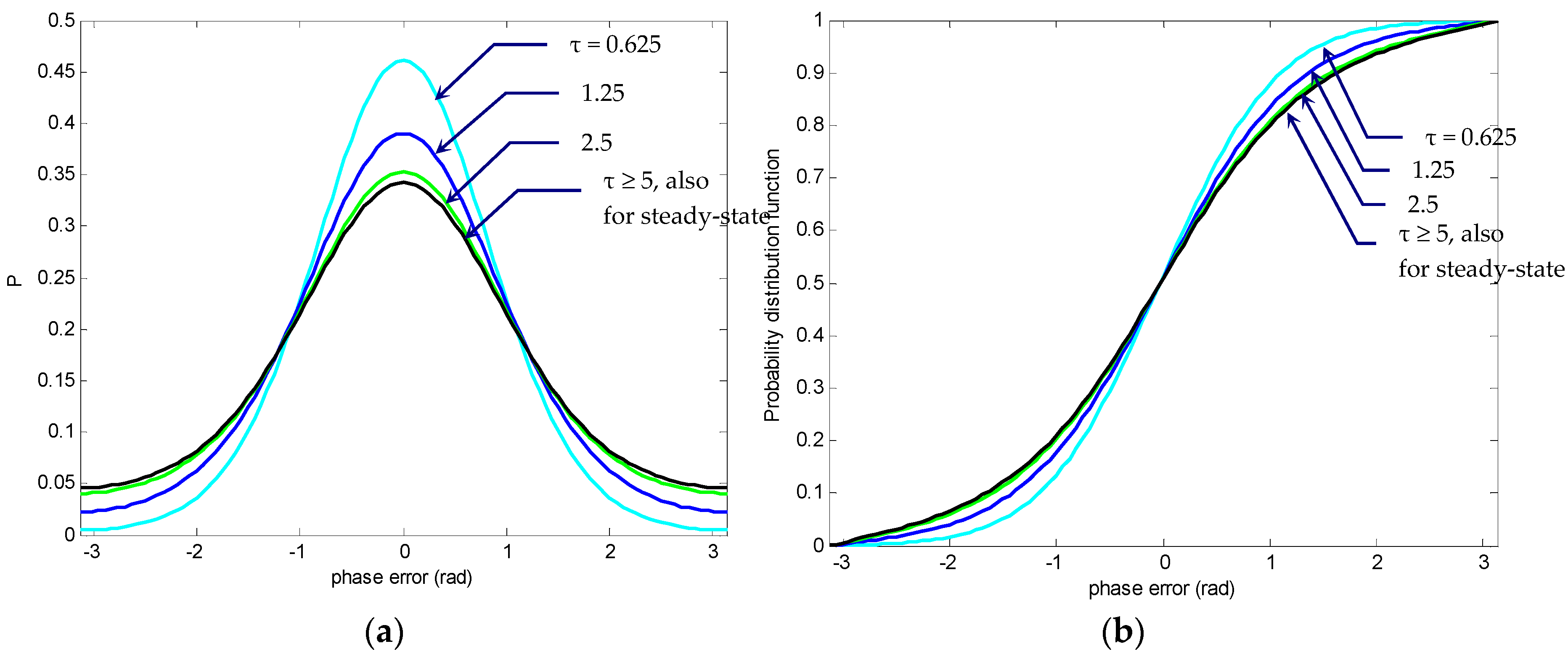
In the following discussion, the modulo-2π PDF, $P(\varphi ,\tau )$ (denoted by a capital letter P) as well as the cumulative probability distribution, and the cycle slipping density function $q(\varphi ,\tau )$ of the phase error for the first-order PLL are presented. The time-evolution of modulo-2π phase-error PDF $P(\varphi ,\tau )$ and cumulative probability distribution is shown in Figure 17. In this illustrative example, the SNR $\alpha =1$ and detuning factor $\gamma =0$ were utilized. The numbers beside individual curves indicate the normalized times, switching τ from 0.625 to 5. The steady state was reached when the normalized time $\tau \ge 5$. Since the total time steps for simulation were set as 1000, the grid spacing in the time marching direction was $\Delta \tau =\tau /1000$, which is dependent on the normalized time τ. As time τ progressed, the peak value of $P(\varphi ,\tau )$ at zero phase error ($\varphi =0$) was decreasing, while remaining symmetric with respect to the phase-error axis.

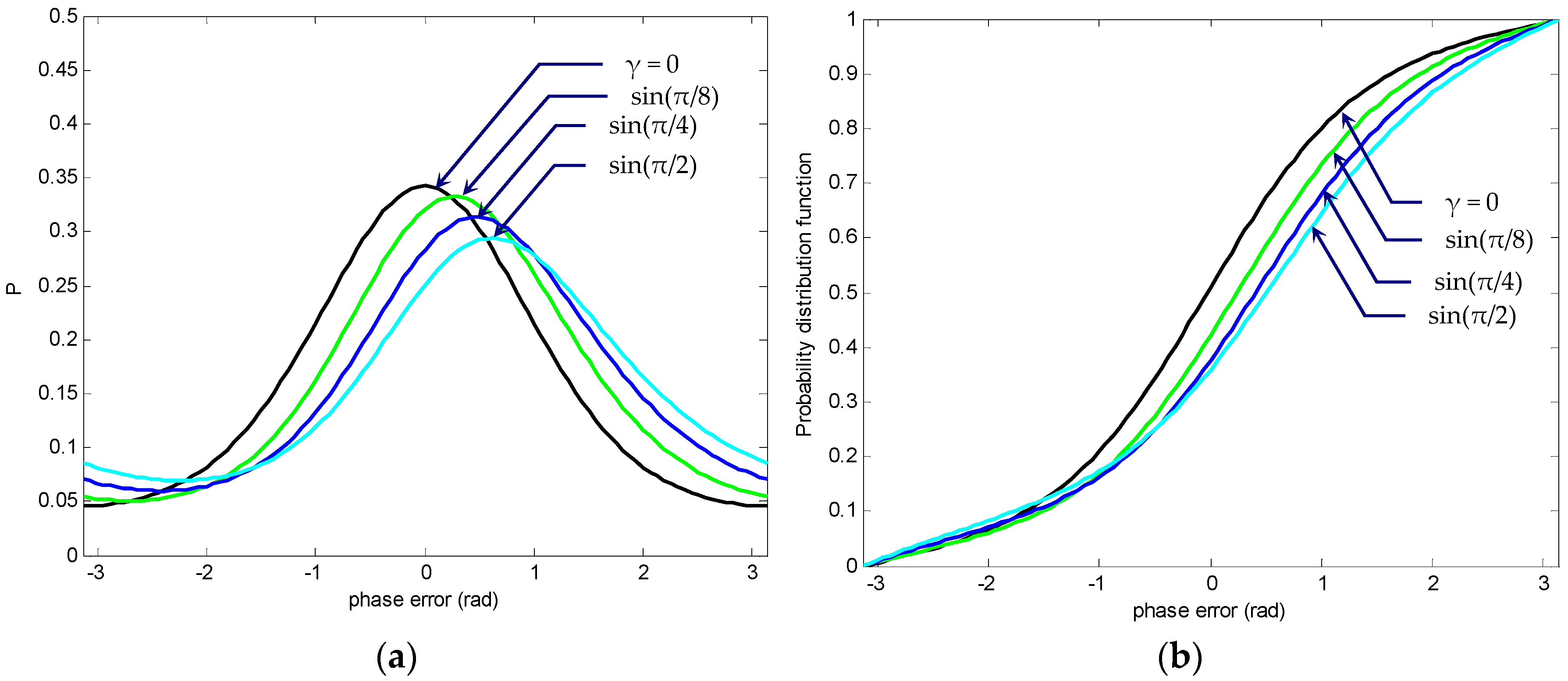
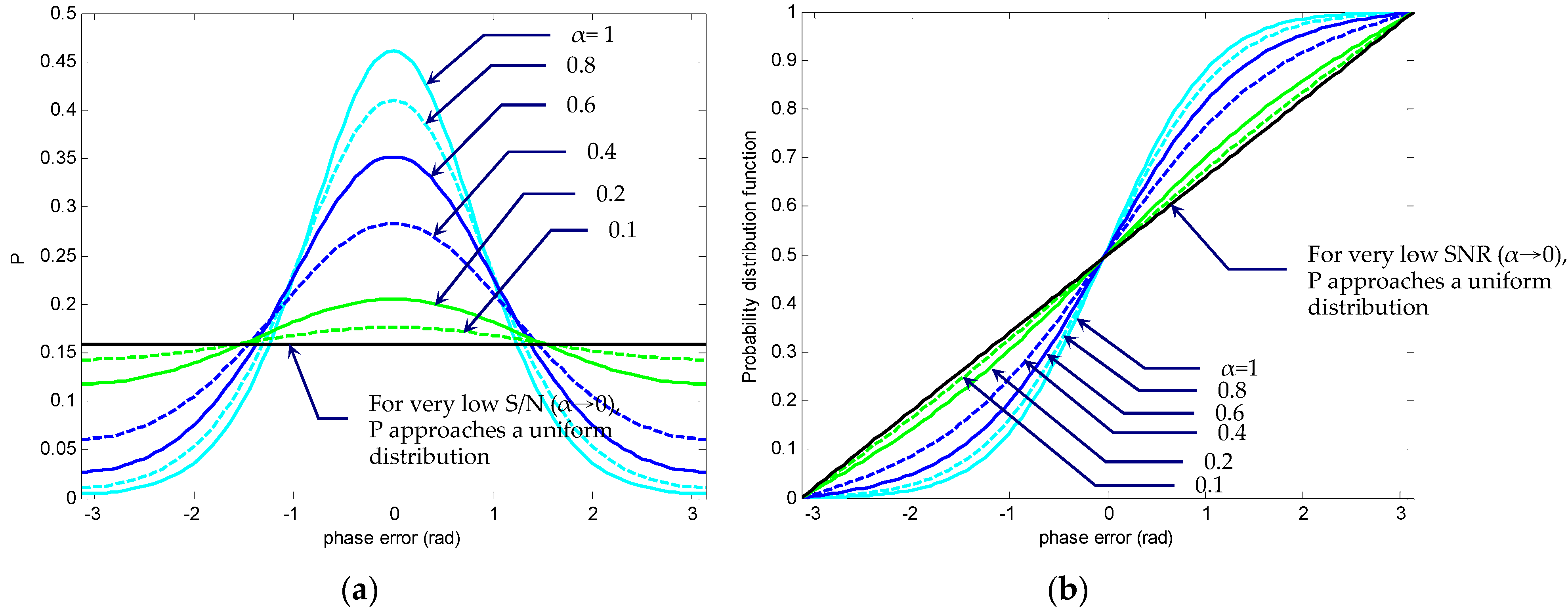
Figure 18 provides the comparison on variation of modulo-2π phase-error steady state PDF $P(\varphi )$ and cumulative probability distribution function for various detuning factor $\gamma$ where SNR $\alpha =1$ was utilized. The numbers beside individual curves indicate the detuning factors in the range 0–$\sin (\pi /2)$. It can be seen that, initially with a symmetric shape, $P(\varphi )$ became the left-skewed distribution. The peak moved rightwards with its amplitude decreasing as $\gamma$ increased. Figure 19 provides the variation of modulo-2π phase-error steady state PDF and cumulative probability distribution function, respectively, of the phase error at τ = 0.625 for the SNR values α in the range 0–1 in the case of $\gamma =0$. The numbers beside individual curves indicate the SNR values α. It can be seen that, the peak value of $P(\varphi )$ appeared at $\varphi =0$ and was monotonically decreasing, while remaining symmetric with respect to the phase-error axis as α was increased. For a very high SNR ($\alpha =1$),$P(\varphi )$ resembled a unity Gaussian distribution, while for very low SNR ($\alpha \to 0$), it became flat and approached a uniform distribution from –π to π, with the PDF $P(\varphi )=1/(2\pi \mathrm{rad})$, implying that the phase was completely unknown.

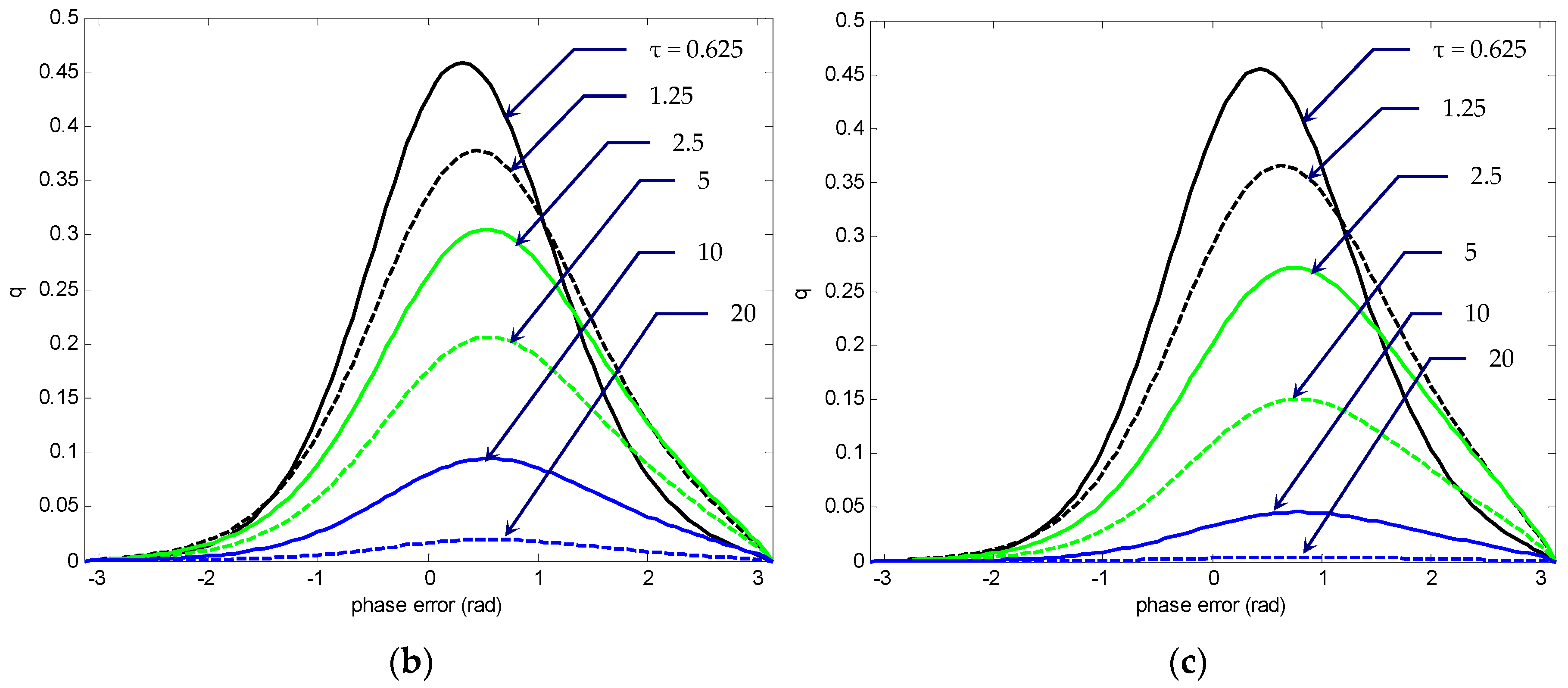
The function $q(\varphi ,\tau )$ for the primary cycle slip was essentially identical to the $p(\varphi ,\tau )$ function until a significant amount of probability mass was lost at the absorbing boundaries at $\varphi =\pm \pi$. The inclusion of absorbing boundaries around some subinterval of $\varphi$, e.g., [−π, π], enabled one to determine the probability that the phase error had not yet exceeded the limits of that subinterval at any prior time. The end points were held at zero to simulate the effect of the slip boundary. Figure 20 shows the time-evolution of primary cyclic slipping density function $q(\varphi ,\tau )$. The curves were plotted for the conditions SNR $\alpha =1$, where three values of detuning factor, $\gamma =0$, $\sin (\pi /4)$ and $\sin (\pi /2)$, respectively, are depicted.

The results provide us a meaningful conceptual link between the stochastic process and information geometry. Through the above examples of physical realizations, the results underscore the natural, intuitive interpretation of information profiles and changes associated with the stochastic process in the phase-locked loop, and can be utilized for optimizing various desired outcomes.

5. Conclusions

Information geometry of the phase-error statistics for the first-order phase-locked loop was presented. A thorough parameter study of PDFs for different values of the PLL parameters was presented by solving the Fokker–Planck equation numerically. Due to the fact that the modified Fokker–Planck equation bears a very good analogy with the transport equation, the numerical algorithms were derived for the transport equation and then applied to solve the Fokker–Planck equation. The implicit Crank–Nicolson finite-difference method was employed in that it is computationally advantageous in terms of both accuracy and stability.

Illustrative examples include the transient and stationary statistics for the nonmodulo-2π probability density functions and cumulative probability distribution functions, modulo-2π probability density functions and probability distribution functions, and cycle slipping density function of the phase error, with various settings of parameters involved, including the detuning factor γ and SNR α. The property of skewness on the probability density/histogram due to the non-zero detuning factor γ was discussed. Additionally, shown for the nonmodulo-2π PLL statistics were the three-dimensional plots for g and p, respectively, of the phase error for profound insights into the PLL behavior. As for the modulo-2π statistics, the time-evolutions of phase-error PDF and cumulative probability distribution function, respectively, were shown. Comparison on the variation of steady-state modulo-2π phase-error statistics, for a specific SNR with various detuning factors was presented. Furthermore, variation of modulo-2π statistics of the phase error for various SNR values was also involved. Furthermore, the time-evolution of cyclic slipping density function for varying detuning factor was addressed.

The results presented in this paper provided comprehensive treatment and elucidated the statistics of the PLL phase error from different perspectives, qualitatively and quantitatively in some extent, and are useful for future PLL investigation and designs.

References

1. Spilker, J.J. Digital Communications by Satellite; Prentice-Hall: Englewood Cliffs, NJ, USA, 1977. [Google Scholar]
2. Egan, W.F. Phase-Lock Basics; John Wiley & Sons: New York, NY, USA, 1998. [Google Scholar]
3. Gardner, F.M. Phaselock Techniques, 2nd ed.; John Wiley & Sons: New York, NY, USA, 1979. [Google Scholar]
4. Spilker, J.J., Jr. Fundamentals of Signal Tracking Theory. In Global Positioning System Theory and Applications; Parkinson, B.W., Spilker, J.J., Jr., Eds.; AIAA, Inc.: Washington, DC, USA, 1996; Volume I, Chapter 7; pp. 245–327. [Google Scholar]
5. Van Dierendonck, A.J. GPS Receivers. In Global Positioning System Theory and Applications; Parkinson, B.W., Spilker, J.J., Jr., Eds.; AIAA, Inc.: Washington, DC, USA, 1996; Volume I, Chapter 8; pp. 329–407. [Google Scholar]
6. Kaplan, E.D. (Ed.) Understanding GPS: Principles and Applications; Artech House Publishers: Boston, MA, USA, 1996. [Google Scholar]
7. Borre, K.; Akos, D.; Bertelsen, N.; Rinder, P.; Jensen, S.H. A Software-Defined GPS and Galileo Receiver: A Single-Frequency Approach; Springer: New York, NY, USA, 2007. [Google Scholar]
8. Tsui, J.B.Y. Global Positioning System Receivers: A Software Approach; John Wiley & Sons: New York, NY, USA, 2000. [Google Scholar]
9. Pospelov, S.S.; Botchkovski, A.L.; Krauss P., A.; Berberich, S. GNSS Software Receiver. GPS Solut. 2000, 4, 48–55. [Google Scholar] [CrossRef]
10. Viterbi, A.J. Phase-Locked Loop Dynamics in the presence of noise by Fokker-Planck Techniques. Proc. IEEE 1963, 51, 1737–1754. [Google Scholar] [CrossRef] [Green Version]
11. Zhang, W. An analytical solution of the Fokker-Planck equation in the Phase-Locked Loop Transient Analysis. IEEE Trans. Commun. 1987, 35, 773–775. [Google Scholar] [CrossRef]
12. Zorzano, M.P.; Mais, H.; Vazquez, L. Numerical solution of two dimensional Fokker-Planck equations. Appl. Math. Comput. 1999, 98, 109–117. [Google Scholar] [CrossRef]
13. Challa, S. Nonlinear filter design using Fokker-Planck-Kolmogorov probability density evolutions. IEEE Trans. Aerosp. Electron. Syst. 2000, 36, 309–315. [Google Scholar] [CrossRef]
14. Frank, T.D. Linear and nonlinear Fokker-Planck Equations. In Encyclopedia of Complexity and Systems Science; Meyers, R.A., Ed.; Springer Science+Business Media LLC: Berlin, Germany, 2017. [Google Scholar] [CrossRef]
15. Fletcher, C.A. Computational Techniques for Fluid Dynamics, 2nd ed.; Springer: New York, NY, USA, 1991; Volume I. [Google Scholar]
16. Ferziger, J.H.; Peric, M. Computational Methods for Fluid Dynamics, 3rd ed.; Springer: New York, NY, USA, 1993. [Google Scholar]
17. Tannehill, J.C.; Anderson, D.A.; Pletcher, R.H. Computational Fluid Mechanics and Heat Transfer, 2nd ed.; Taylor & Francis: Philadelphia, PA, USA, 1997. [Google Scholar]
18. Hoffmann, K.A.; Chiang, S.T. Computational Fluid Dynamics for Engineers; Engineering Publishing System: Wichita, KS, USA, 1993; Volume I. [Google Scholar]
19. Ames, W.F. Numerical Methods for Partial Differential Equations; Academic Press: San Diego, CA, USA, 1992. [Google Scholar]
20. Lapidus, L.; Pinder, G.F. Numerical Solution of Partial Differential Equations in Science and Engineering; John Wiley & Sons: New York, NY, USA, 1982. [Google Scholar]
21. Hollerbach, R.; Dimanche, D.; Kim, E.-J. Information Geometry of Nonlinear Stochastic Systems. Entropy 2018, 20, 550. [Google Scholar] [CrossRef] [Green Version]
22. Jacquet, Q.; Kim, E.-J.; Hollerbach, R. Time-Dependent Probability Density Functions and Attractor Structure in Self-Organised Shear Flows. Entropy 2018, 20, 613. [Google Scholar] [CrossRef] [Green Version]
23. Hollerbach, R.; Kim, E.-J.; Mahi, Y. Information length as a new diagnostic in the periodically modulated double-well model of stochastic resonance. Phys. A: Stat. Mech. Its Appl. 2019, 525, 1313–1322. [Google Scholar] [CrossRef] [Green Version]
24. Kim, E.-J.; Jacquet, Q.; Hollerbach, R. Information geometry in a reduced model of self-organised shear flows without the uniform coloured noise approximation. J. Stat. Mech.: Theory Exp. 2019, 2019, 023204. [Google Scholar] [CrossRef] [Green Version]
25. Hollerbach, R.; Kim, E.-J. Information Geometry of Spatially Periodic Stochastic Systems. Entropy 2019, 21, 681. [Google Scholar] [CrossRef] [Green Version]
26. Kim, E.; Hollerbach, R. Time-dependent probability density function in cubic stochastic processes. Phys. Rev. E 2016, 94, 052118. [Google Scholar] [CrossRef] [PubMed] [Green Version]
27. Guérin, T.; Dean, D.S. Universal time-dependent dispersion properties for diffusion in a one-dimensional critically tilted potential. Phys. Rev. E 2017, 95, 012109. [Google Scholar] [CrossRef] [PubMed] [Green Version]
28. Dominak, K.E.; Pickholtz, R.L. Transient behavior of a phase-locked loop in the presence of noise. IEEE Trans. Commun. 1970, 18, 452–456. [Google Scholar] [CrossRef]
29. Jwo, D. Implicit methods for solving PLL transient statistics. Information 2014, 17, 2487–2507. [Google Scholar]
30. Ohlson, J.E.; Rutherford, A. Transient statistics of the first-order phase-locked loop. IEEE Trans. Commun. 1974, 22, 698–703. [Google Scholar] [CrossRef]
31. Brunt, S.M.; Darnell, M.; Grayson, M. Cycle-slipping probability of first-order phase-locked loop using transient analysis. IEEE Proc.-Commun. 1997, 144, 357–360. [Google Scholar] [CrossRef]
32. Anders, J.; Mathis, W. Noise analysis of phase locked loops using stochastic differential equations. In Proceedings of the 5th Vienna Conference on Mathematical Modelling, Vienna, Austria, 8–10 February 2006. [Google Scholar]
33. Mehrotra, A. Noise analysis of phase-locked loops. IEEE Trans. Circuits Syst.-I Fundam. Theory Appl. 2002, 49, 1309–1316. [Google Scholar] [CrossRef]
Figure 1. Mathematical block diagram of the phase-locked loop (PLL). The basic PLL configuration contains a phase detector (PD), for detecting the phase error between the output and the input through feedback system; a loop filter; and a voltage-controlled oscillator (VCO). The loop filter F ( s ) is usually a low-pass filter used to suppress the noise and high-frequency signal components from the phase-detector/delay discriminator and provide a dc-controlled signal for the VCO [1,2,3].
Applsci 10 02625 g001
Figure 2. The time-evolution of the nonmodulo-2π (a) density function g ( ϕ , τ ) and (b) PDF p ( ϕ , τ ) , of the phase error for the signal-to-noise ratio (SNR) α = 1 ( γ = 0 ).
Applsci 10 02625 g002
Figure 3. The time-evolution of the nonmodulo-2π cumulative probability distribution of the phase error for SNR α = 1 ( γ = 0 ).
Applsci 10 02625 g003
Figure 4. Three-dimensional plots for nonmodulo-2π transition g and p, respectively, for SNR α = 1 as time progresses: front view (left) and back view (right) ( γ = 0 ).
Applsci 10 02625 g004
Figure 5. The time-evolution of the nonmodulo-2π (a) density function g ( ϕ , τ ) and (b) PDF p ( ϕ , τ ) , of the phase error for SNR α = 1 ( γ = sin ( π / 4 ) ).
Applsci 10 02625 g005
Figure 6. The time-evolution of the nonmodulo-2π cumulative probability distribution of the phase error for SNR α = 1 ( γ = sin ( π / 4 ) ).
Applsci 10 02625 g006
Figure 7. Three-dimensional plots for the nonmodulo-2π transition g and p, respectively, for SNR α = 1 as time progresses: front view (left) and back view (right; γ = sin ( π / 4 ) ).
Applsci 10 02625 g007
Figure 8. Nonmodulo-2π phase-error (a) density function g ( ϕ , τ ) and (b) PDF p ( ϕ , τ ) , at τ = 10 for various SNR values ( γ = 0 ).
Applsci 10 02625 g008
Figure 9. Nonmodulo-2π phase-error cumulative probability distribution at τ = 10 for various SNR values ( γ = 0 ).
Applsci 10 02625 g009
Figure 10. Three-dimensional plots for nonmodulo-2π g and p, respectively, at τ = 10 for various SNR values: front view (left) and back view (right; γ = 0 ).
Applsci 10 02625 g010
Figure 11. Nonmodulo-2π phase-error (a) density function g ( φ , τ ) and (b) PDF p ( ϕ , τ ) , at τ = 10 for various SNR values ( γ = sin ( π / 4 ) ).
Applsci 10 02625 g011
Figure 12. Nonmodulo-2π phase-error cumulative probability distribution at τ = 10 for various SNR values ( γ = sin ( π / 4 ) ).
Applsci 10 02625 g012
Figure 13. Three-dimensional plots for nonmodulo-2π g and p, respectively, at τ = 10 for various SNR values: front view (left) and back view (right; γ = sin ( π / 4 ) ).
Applsci 10 02625 g013
Figure 14. Nonmodulo-2π phase-error (a) density function g ( ϕ , τ ) and (b) PDF p ( ϕ , τ ) , at τ = 10 for various detuning factor γ when SNR α = 1 .
Applsci 10 02625 g014
Figure 15. Nonmodulo-2π phase-error cumulative probability distribution at τ = 10 for various detuning factors γ when SNR α = 1 .
Applsci 10 02625 g015
Figure 16. Three-dimensional plots for nonmodulo-2π g and p, respectively, at τ = 10 for various detuning factors γ when SNR α = 1 : front view (left) and back view (right).
Applsci 10 02625 g016
Figure 17. The time-evolution of modulo-2π phase-error: (a) PDF, P ( ϕ , τ ) and (b) cumulative probability distribution function, for SNR α = 1 ( γ = 0 ).
Applsci 10 02625 g017
Figure 18. Variation of modulo-2π phase-error steady state: (a) PDF and (b) cumulative probability distribution function, for SNR α = 1 with various detuning factors γ ( τ 5 or steady-state).
Applsci 10 02625 g018
Figure 19. Variation of modulo-2π phase-error steady state: (a) PDF and (b) cumulative probability distribution function at τ = 0.625 for various SNR values ( γ = 0 ).
Applsci 10 02625 g019
Figure 20. The time-evolution of primary cyclic slipping density function q ( ϕ , τ ) for SNR α = 1 : (a) γ = 0 ; (b) γ = sin ( π / 4 ) ; and (c) γ = sin ( π / 2 ) .
Applsci 10 02625 g020aApplsci 10 02625 g020b