Asymptotic Performance Analysis of Maximum Likelihood Algorithm for Direction-of-Arrival Estimation: Explicit Expression of Estimation Error and Mean Square Error

Abstract

This paper proposes a new method to get explicit expressions of some quantities associated with performance analysis of the maximum likelihood DOA algorithm in the presence of an additive Gaussian noise on the antenna elements. The motivation of the paper is to make a quantitative analysis of the ML DOA algorithm in the case of multiple incident signals. We present a simple method to derive a closed-form expression of the MSE of the DOA estimate based on the Taylor series expansion. Based on the Taylor series expansion and approximation, we get explicit expressions of the MSEs of estimates of azimuth angles of all incident signals. The validity of the derived expressions is shown by comparing the analytic results with the simulation results.

1. Introduction

There has been a lot of research on the direction-of-arrival (DOA) estimation [1,2,3,4,5,6,7,8,9,10,11,12,13,14,15,16,17,18,19]. Our interest in this paper is the performance analysis of the maximum likelihood (ML)-based DOA estimation algorithm.

In [8], a performance analysis of the ML DOA estimation algorithm for low SNR and small number of snapshots is considered. A threshold effect in the ML DOA algorithm is exploited, and the authors derive approximations to the mean square error and probability of outlier.

If the noise variance at each sensor in the array antenna system is equal, the noise covariance matrix is considered to be multiples of an identity matrix. In [9], nonuniform white noise, whose covariance matrix can be expressed as an arbitrary diagonal covariance, is considered, and the new ML DOA algorithm for nonuniform noise is proposed, and the performance analysis of the proposed algorithm is also presented.

In [10], the authors addressed the DOA estimation using sparse sensor arrays, where the sensor noises can be uncorrelated between different subarrays due to large intersubarray spacings. The authors proposed a new maximum-likelihood estimator, which can be extended to the uncalibrated arrays with sensor gain and phase mismatch.

A new computationally efficient ML DOA algorithm exploiting spatial aliasing is proposed in [11]. Generally, spatial aliasing is undesirable since it degrades the DOA estimation accuracy. In [11], the authors adopted a nested array structure with a doubly spaced aperture. The computational burden of the ML DOA estimation algorithm is reduced by the highly compressed search range and the small number of candidate angles to be searched. The authors also presented Monte Carlo simulation based mean square error (MSE). However, analytic performance analysis of the proposed scheme is not presented in [11].

A new ML DOA algorithm for use with a uniform linear array is proposed [12]. The scheme is superior to the conventional ML algorithm when the true DOAs of two incident signals are very close to each other. The formulation for the new DOA algorithm is based on an asymptotic approximation of the unconditional maximum likelihood (UML) procedure when two closely space signals are incident on the ULA. Taylor approximation is also adopted for derivation of the new algorithm. Empirical MSE is illustrated to validate the proposed scheme. However, the authors do not present analytic performance analysis of the new DOA algorithm.

To overcome the problem of large computational complexity for implementation of the ML DOA estimation algorithm, based on a spatially overcomplete array output formulation, an efficient ML DOA estimator is proposed in [13]. Empirical performance from Monte Carlo simulation is present to illustrate the superiority of the proposed scheme over the other DOA algorithms. Analytic performance analysis is not given.

Although the ML estimator is known to be optimal in DOA estimation, its computational cost can be quite prohibitive, especially for a large number of incident signals. To solve this problem, in [14], three kinds of natural computing algorithms, differential evolution, clonal selection algorithm, and the particle swarm optimization, are applied for implementation of the multivariable nonlinear optimization of the cost function of the ML DOA estimation algorithm. It turns out that all three natural computing algorithms are capable of optimizing the ML DOA cost function, irrespective of the number of incident signals and their nature. In addition, the number of points evaluated by natural computing algorithms is much smaller than that associated with exhaustive grid search-based algorithms, justifying the application of these natural computing algorithms to the optimization of the cost function of the ML DOA estimation algorithm.

In [15], a new implementation of ML DOA estimation, which outperforms the other DOA algorithms for closely spaced incident signals, is proposed. The concept of Monte Carlo importance sampling is applied. The superiority of the proposed scheme comes from its better convergence to a global maximum in comparison with other iterative approaches. Although analytical performance analysis of the proposed scheme is not presented, empirical performance of the propose algorithm and the other DOA algorithms is given. Note that Monte Carlo simulation is employed to get empirical performance in terms of the MSE of the DOA estimate.

A heuristic optimization algorithm, called gravitational search algorithm, is presented to optimize the cost function of the ML DOA estimation algorithm for a uniform circular array [16]. It is empirically shown that the proposed algorithm is superior to the MUSIC algorithm and particle swarm optimization-based ML algorithm. Analytic performance analysis of the proposed scheme is not presented in [16].

To reduce computational burden of optimizing the cost function of ML DOA estimation algorithm, the artificial bee colony (ABC) algorithm is applied to maximize the cost function of the ML DOA estimation algorithm [17]. It is empirically shown that the proposed scheme is superior to other ML-based DOA estimation methods in the view point of efficiency in computation and statistical performance. Analytic performance analysis of the proposed scheme is not presented in [17].

DOA estimation of narrowband sources in unknown nonuniform white noise is considered in [18]. The stepwise concentration of the log-likelihood function with respect to the signal parameters and noise parameters is obtained by alternating minimization of the Kullback–Leibler divergence. Closed-form expressions for the signal parameters and noise parameters are derived, implying that the proposed scheme results in significant reduction in computational complexity in comparison with exhaustive multidimensional search-based ML DOA algorithms.

In [19], a new wideband ML DOA estimation algorithm for an unknown nonuniform sensor noise is proposed to reduce the performance degradation due to nonuniformity of the noise. Two associated implementation schemes are proposed: one is iterative and the other is non-iterative. Simulation results show that the performance of two processing algorithms is consistent with the Cramer–Rao lower bound. Analytic performance analysis, more specifically the Cramer–Rao lower bound, of the proposed algorithm is presented in [19].

In this paper, we are concerned with quantitative study on how much estimation error is induced due to an additive Gaussian noise on array antennas. More specifically, mean-squared error (MSE) of direction-of-arrival estimation in terms of a standard deviation of an additive noise is derived. In this paper, performance analysis of azimuth estimation using uniform linear array (ULA) is presented.

In this paper, the estimate with no superscript denotes the estimate of the original ML algorithm. Note that no approximation is used in getting the estimate with no superscript. In this paper, the estimate with the superscript $(u=1)$ denotes the estimate by using the first approximation, and that with the superscript $(u=1,v)$ represents the estimate by using the first approximation and the second approximation.

The difference between the estimate with no superscript and the estimate with the superscript $(u=1)$ quantifies the error due to the first approximation since the first approximation is applied in getting the estimate with the superscript $(u=1)$. Note that no approximation is applied in getting the estimate with no superscript. Similarly, the difference between the estimate with the superscript $(u=1)$ and the estimate with the superscript $(u=1,v)$ quantifies the error due to the second approximation since the first approximation and the second approximations are applied in getting the estimate with the superscript $(u=1,v)$. Based on this intuition, by comparing these three estimates, we can easily determine which approximation results in the dominant approximation error. This inspection cannot be obtained from the scheme presented in the previous study [7,8,9,19].

In this paper, Gaussian noise is used to model measurement uncertainty. The effect of Gaussian noise on the accuracy of the azimuth estimate is rigorously derived. Furthermore, an explicit expression of the MSE of the azimuth estimate is also derived. In comparison with the previous studies on the performance analysis of the maximum likelihood algorithm [7,8,9,19], a more explicit representation of the MSE of the azimuth estimate is proposed in this paper.

Many previous studies on the ML DOA estimation algorithm focused on how the performance of the ML DOA estimation algorithm can be improved by proposing new algorithms or by modifying the ML DOA estimation algorithm [9,10,11,12,13,14,15,16,17,18,19]. Note that our contribution in this paper does not lie in how much improvement can be achieved by proposing an improved ML DOA algorithm. Our contribution lies in a reduction in computational cost in getting the MSE of an existing ML DOA algorithm by adopting an analytic approach, rather than the Monte Carlo simulation-based MSE under measurement uncertainty which is assumed to be Gaussian distributed. That is, the scheme described how analytic MSE can be obtained with much less computational complexity than the Monte Carlo simulation-based MSE.

In this paper, the derivation is based on the Taylor series expansion of the sample covariance matrix since the cost function of the ML DOA estimation algorithm can be explicitly written in terms of the sample covariance matrix. The difference between the sample covariance matrix associated with noisy measurement and that associated with noiseless sample covariance matrix is explicitly expressed in terms of additive noises on the antenna arrays. Azimuth estimation error is explicitly expressed in terms of the additive noises. Finally, the MSE of the azimuth estimate is given in terms of the statistics of an additive noise. To the best of our knowledge, no previous study presented these explicit expressions of the azimuth estimation error and the MSE of the azimuth estimate in terms of the statistics of an additive noise.

The proposed scheme can be used in predicting how accurate the estimate of the ML DOA estimation algorithm is without a computationally intensive Monte Carlo simulation. The performance of the ML algorithm depends on various parameters including the number snapshots, the number antenna elements in the array, inter-element spacing between adjacent antenna elements, and the SNR. Therefore, Monte Carlo simulations for different values of the various parameters can be computationally intensive. Therefore, the scheme presented in this paper can be adopted to predict the accuracy of the ML DOA algorithm for different values of various parameters.

2. Maximum Likelihood Algorithm

In this section, the maximum likelihood (ML) for use with the uniform linear array (ULA) algorithm is briefly described.

In the case of ULA, for the incident signal from ${\theta }_c$, the array vector associated with the m-th antenna can be written as

$$a_m\left({\theta }_c\right)=exp\left[j\frac{2\pi }{\lambda }\left(m-1\right)\Delta sin{\theta }_c\right],$$

(1)

where $\lambda$ is wavelength and $\Delta$ is the distance between two neighboring elements.

Using (1), $\mathbf{A}\left({\theta }_1,{\theta }_2,\cdots ,{\theta }_d\right)$ is defined as

$$\mathbf{A}\left({\theta }_1,{\theta }_2,\cdots ,{\theta }_d\right)=\left[\begin{array}{cccc}{a}_1\left({\theta }_1\right)& a_1\left({\theta }_2\right)& \cdots & a_1\left({\theta }_d\right)\\ ⋮& ⋮& \ddots & ⋮\\ a_M\left({\theta }_1\right)& a_M\left({\theta }_2\right)& \cdots & a_M\left({\theta }_d\right)\end{array}\right]$$

(2)

where the number of incident signals is d.

Projection matrix on to the column space of $\mathbf{A}\left({\theta }_1,{\theta }_2,\cdots ,{\theta }_d\right)$ can be expressed as [6]

$${\mathbf{P}}_{\mathbf{A}\left({\theta }_1,{\theta }_2,\cdots ,{\theta }_d\right)}=\mathbf{A}\left({\theta }_1,{\theta }_2,\cdots ,{\theta }_d\right){\left(\mathbf{A}{\left({\theta }_1,{\theta }_2,\cdots ,{\theta }_d\right)}^H\mathbf{A}\left({\theta }_1,{\theta }_2,\cdots ,{\theta }_d\right)\right)}^{-1}\mathbf{A}{\left({\theta }_1,{\theta }_2,\cdots ,{\theta }_d\right)}^H.$$

(3)

The incident signals on the array antenna elements can be written as, for $i=1,\cdots ,L$,

$$\begin{array}{l}\hfill \begin{array}{c}\mathbf{x}\left(t_i\right)=\mathbf{A}\left({\theta }_1,{\theta }_2,\cdots ,{\theta }_d\right)\mathbf{s}\left(t_i\right)\hfill \\ \left[\begin{array}{c}{x}_1\left(t_i\right)\\ ⋮\\ x_M\left(t_i\right)\end{array}\right]=\mathbf{A}\left({\theta }_1,{\theta }_2,\cdots ,{\theta }_d\right)\left[\begin{array}{c}{s}_1\left(t_i\right)\\ s_2\left(t_i\right)\\ ⋮\\ s_d\left(t_i\right)\end{array}\right].\hfill \end{array}\end{array}$$

(4)

The noisy incident signals can be expressed as

$$\begin{array}{lll}\hfill {\mathbf{x}}^{\prime }\left(t_i\right)& =& \mathbf{A}\left({\theta }_1,{\theta }_2,\cdots ,{\theta }_d\right)\mathbf{s}\left(t_i\right)+\mathbf{n}\left(t_i\right)\hfill \\ \hfill \left[\begin{array}{c}{x}_1^{\prime }\left(t_i\right)\\ ⋮\\ x_M^{\prime }\left(t_i\right)\end{array}\right]& =& \mathbf{A}\left({\theta }_1,{\theta }_2,\cdots ,{\theta }_d\right)\left[\begin{array}{c}{s}_1\left(t_i\right)\\ s_2\left(t_i\right)\\ ⋮\\ s_d\left(t_i\right)\end{array}\right]+\left[\begin{array}{c}{n}_1\left(t_i\right)\\ ⋮\\ n_M\left(t_i\right)\end{array}\right].\hfill \end{array}$$

(5)

It is assumed that the entries of the Gaussian vector are independent and identically distributed Gaussian random variables with the same mean and the same variance. Note that the noise are complex-valued and that the real part and the imaginary part of the noise are independent Gaussian random variables with non-zero mean $\mu$. The variance of the real part is denoted by $\frac{{\sigma }^2}{2}$, which is equal to the variance of the imaginary part,$\frac{{\sigma }^2}{2}$.

Let L denote the number of the snapshots. $\widehat{\mathbf{R}}$ is a sample covariance matrix given by

$$\widehat{\mathbf{R}}=\frac{1}{L}{\displaystyle \sum _{t_i=1}^L}\left\{\mathbf{x}\left(t_i\right)\mathbf{x}{\left(t_i\right)}^H\right\}=\left[\begin{array}{ccc}{\widehat{R}}_{11}& \cdots & {\widehat{R}}_{1M}\\ ⋮& \ddots & ⋮\\ {\widehat{R}}_{M1}& \cdots & {\widehat{R}}_{MM}\end{array}\right]$$

(6)

where $\mathbf{x}\left(t_i\right)$ is given by (4).

From (5), we get

$${\widehat{\mathbf{R}}}^{\prime }=\frac{1}{L}{\displaystyle \sum _{t_i=1}^L}\left\{{\mathbf{x}}^{\prime }\left(t_i\right){\mathbf{x}}^{\prime }{\left(t_i\right)}^H\right\}=\left[\begin{array}{ccc}{\widehat{R}}_{11}^{\prime }& \cdots & {\widehat{R}}_{1M}^{\prime }\\ ⋮& \ddots & ⋮\\ {\widehat{R}}_{M1}^{\prime }& \cdots & {\widehat{R}}_{MM}^{\prime }\end{array}\right].$$

(7)

$\delta \mathbf{R}$ is defined as

$$\delta \mathbf{R}={\widehat{\mathbf{R}}}^{\prime }-\widehat{\mathbf{R}}.$$

(8)

In the ML algorithm, the estimates, $\left[{\widehat{\theta }}_1,{\widehat{\theta }}_2,\cdots ,{\widehat{\theta }}_d\right]$, are obtained from

$$\left[{\widehat{\theta }}_1,{\widehat{\theta }}_2,\cdots ,{\widehat{\theta }}_d\right]=arg\left(\underset{{\theta }_1,{\theta }_2,\cdots ,{\theta }_d}{max}\left[\mathrm{tr}\left({\mathbf{P}}_{\mathbf{A}\left({\theta }_1,{\theta }_2,\cdots ,{\theta }_d\right)}{\widehat{\mathbf{R}}}^{\prime }\right)\right]\right),$$

(9)

where ${\widehat{\theta }}_c$ is given by ${\widehat{\theta }}_c={\theta }_c^{\left(0\right)}+\delta {\theta }_c$$\left(c=1,\cdots ,d\right)$, and $\mathrm{tr}\left({\mathbf{P}}_{\mathbf{A}\left({\theta }_1,{\theta }_2,\cdots ,{\theta }_{\mathrm{d}}\right)}{\widehat{\mathbf{R}}}^{\prime }\right)$ can be written as

$$\begin{array}{ccc}\hfill \mathrm{tr}\left({\mathbf{P}}_{\mathbf{A}\left({\theta }_1,{\theta }_2,\cdots ,{\theta }_d\right)}{\widehat{\mathbf{R}}}^{\prime }\right)& =& \mathrm{tr}\left(\left[\begin{array}{ccc}{P}_{11}\left({\theta }_1,{\theta }_2,\cdots ,{\theta }_d\right)& \cdots & P_{1M}\left({\theta }_1,{\theta }_2,\cdots ,{\theta }_d\right)\\ ⋮& \ddots & ⋮\\ P_{M1}\left({\theta }_1,{\theta }_2,\cdots ,{\theta }_d\right)& \cdots & P_{MM}\left({\theta }_1,{\theta }_2,\cdots ,{\theta }_d\right)\end{array}\right]\left[\begin{array}{ccc}{\widehat{R}}_{11}^{\prime }& \cdots & {\widehat{R}}_{1M}^{\prime }\\ ⋮& \ddots & ⋮\\ {\widehat{R}}_{M1}^{\prime }& \cdots & {\widehat{R}}_{MM}^{\prime }\end{array}\right]\right)\hfill \\ & =& {\displaystyle \sum _{k=1}^M}{\displaystyle \sum _{l=1}^M}{P}_{kl}\left({\theta }_1,{\theta }_2,\cdots ,{\theta }_d\right){\widehat{R^{\prime }}}_{lk}\hfill \end{array}$$

(10)

where M is the number of antenna elements.

3. Closed-Form Expression of Estimation Error

From (1) and (3), we get

$$a_m\left({\theta }_c\right)\times a_m^{*}\left({\theta }_c\right)=1.$$

(11)

From (11), we obtain

$$\begin{array}{c}\mathbf{A}{\left({\theta }_1,\cdots ,{\theta }_d\right)}^H\mathbf{A}\left({\theta }_1,\cdots ,{\theta }_d\right)\hfill \\ =\left[\begin{array}{ccccc}M& B\left({\theta }_1,{\theta }_2\right)& B\left({\theta }_1,{\theta }_3\right)& \cdots & B\left({\theta }_1,{\theta }_d\right)\\ B^{*}\left({\theta }_1,{\theta }_2\right)& M& B\left({\theta }_2,{\theta }_3\right)& \cdots & B\left({\theta }_2,{\theta }_d\right)\\ B^{*}\left({\theta }_1,{\theta }_3\right)& B^{*}\left({\theta }_2,{\theta }_3\right)& M& \cdots & B\left({\theta }_3,{\theta }_d\right)\\ ⋮& ⋮& & \ddots & ⋮\\ B^{*}\left({\theta }_1,{\theta }_d\right)& B^{*}\left({\theta }_2,{\theta }_d\right)& B^{*}\left({\theta }_3,{\theta }_d\right)& \cdots & M\end{array}\right],\hfill \end{array}$$

(12)

where, from (1), $B({\theta }_k,{\theta }_l)$ is defined as

$$\begin{array}{lll}\hfill B({\theta }_k,{\theta }_l)& \equiv & {\displaystyle \sum _{m=1}^M}exp\left[j\frac{2\pi }{\lambda }\left(m-1\right)\Delta \left(sin{\theta }_l-sin{\theta }_k\right)\right]\hfill \\ & =& \frac{1-exp\left[j\frac{2\pi }{\lambda }\Delta \left(sin{\theta }_l-sin{\theta }_k\right)M\right]}{1-exp\left[j\frac{2\pi }{\lambda }\Delta \left(sin{\theta }_l-sin{\theta }_k\right)\right]}.\hfill \end{array}$$

(13)

Using (12), ${\left({\left(\mathbf{A}{\left({\theta }_1,\cdots ,{\theta }_d\right)}^H\mathbf{A}\left({\theta }_1,\cdots ,{\theta }_d\right)\right)}^{-1}\right)}_{k,l}$ can be written as

$$\begin{array}{l}\hfill \begin{array}{c}{\left({\left(\mathbf{A}{\left({\theta }_1,\cdots ,{\theta }_d\right)}^H\mathbf{A}\left({\theta }_1,\cdots ,{\theta }_d\right)\right)}^{-1}\right)}_{k,l}\hfill \\ =\frac{1}{det\left(\mathbf{A}{\left({\theta }_1,\cdots ,{\theta }_d\right)}^H\mathbf{A}\left({\theta }_1,\cdots ,{\theta }_d\right)\right)}·{\left(\mathrm{adj}\left(\mathbf{A}{\left({\theta }_1,\cdots ,{\theta }_d\right)}^H\mathbf{A}\left({\theta }_1,\cdots ,{\theta }_d\right)\right)\right)}_{k,l}.\hfill \end{array}\end{array}$$

(14)

$\mathrm{adj}\left(·\right)$ denotes adjoint of a matrix. $k,l$-th element of the adjoint of $\mathbf{A}{\left({\theta }_1,\cdots ,{\theta }_d\right)}^H\mathbf{A}\left({\theta }_1,\cdots ,{\theta }_d\right)$ can be expressed as

$$\begin{array}{l}\hfill \begin{array}{c}{\left(\mathrm{adj}\left(\mathbf{A}{\left({\theta }_1,\cdots ,{\theta }_d\right)}^H\mathbf{A}\left({\theta }_1,\cdots ,{\theta }_d\right)\right)\right)}_{k,l}\hfill \\ ={\left(-1\right)}^{k+l}·det\left(\left[\begin{array}{cccccc}M& \cdots & B^{*}\left({\theta }_1,{\theta }_{k-1}\right)& B^{*}\left({\theta }_1,{\theta }_{k+1}\right)& \cdots & B^{*}\left({\theta }_1,{\theta }_d\right)\\ ⋮& \ddots & ⋮& ⋮& & ⋮\\ B\left({\theta }_1,{\theta }_{l-1}\right)& \cdots & B^{*}\left({\theta }_{l-1},{\theta }_{k-1}\right)& B^{*}\left({\theta }_{l-1},{\theta }_{k+1}\right)& \cdots & B^{*}\left({\theta }_{l-1},{\theta }_d\right)\\ B\left({\theta }_1,{\theta }_{l+1}\right)& \cdots & B^{*}\left({\theta }_{l+1},{\theta }_{k-1}\right)& B^{*}\left({\theta }_{l+1},{\theta }_{k+1}\right)& \cdots & B^{*}\left({\theta }_{l+1},{\theta }_d\right)\\ ⋮& & ⋮& ⋮& \ddots & ⋮\\ B\left({\theta }_1,{\theta }_d\right)& \cdots & B\left({\theta }_{k-1},{\theta }_d\right)& B\left({\theta }_{k+1},{\theta }_d\right)& \cdots & M\end{array}\right]\right)\hfill \end{array},\end{array}$$

(15)

where the determinant can be obtained in many ways, one of which is a cofactor expansion.

Generally, the number of incident signals is d. From (14) and (15), an explicit expression of the entry at the k-th row and l-th column of ${\left(\mathbf{A}{\left({\theta }_1,\cdots ,{\theta }_d\right)}^H\mathbf{A}\left({\theta }_1,\cdots ,{\theta }_d\right)\right)}^{-1}$ can be obtained. However, it is very complicated to express the determinant in (15) in terms of the entries of $\mathbf{A}{\left({\theta }_1,\cdots ,{\theta }_d\right)}^H\mathbf{A}\left({\theta }_1,\cdots ,{\theta }_d\right)$ for all $k=1,\cdots ,d$ and $l=1,\cdots ,d$. In addition, due to very complicated expression, expressing each entry of ${\left(\mathbf{A}{\left({\theta }_1,\cdots ,{\theta }_d\right)}^H\mathbf{A}\left({\theta }_1,\cdots ,{\theta }_d\right)\right)}^{-1}$ in terms of the entries of $\mathbf{A}{\left({\theta }_1,\cdots ,{\theta }_d\right)}^H\mathbf{A}\left({\theta }_1,\cdots ,{\theta }_d\right)$ may impair the readability of this paper. Therefore, the number of signals in this paper is set to two.

Using (12) in (3), the entries of ${\mathbf{P}}_{\mathbf{A}\left({\theta }_1,{\theta }_2\right)}$ can be written as

$$\begin{array}{ll}\hfill P_{kl}\left({\theta }_1,{\theta }_2\right)=& \frac{1}{det\left({\theta }_1,{\theta }_2\right)}\left[\left(a_k\left({\theta }_1\right)M-a_k\left({\theta }_2\right)B^{*}\left({\theta }_1,{\theta }_2\right)\right)a_l^{*}\left({\theta }_1\right)\right]\\ & \hfill +\frac{1}{det\left({\theta }_1,{\theta }_2\right)}\left[\left(a_k\left({\theta }_2\right)M-a_k\left({\theta }_1\right)B\left({\theta }_1,{\theta }_2\right)\right)a_l^{*}\left({\theta }_2\right)\right]\end{array}$$

(16)

where $det\left({\theta }_1,{\theta }_2\right)$ is given in Appendix B.

The numerator of $P_{kl}\left({\theta }_1,{\theta }_2\right)$ is defined as $Q_{kl}\left({\theta }_1,{\theta }_2\right)$:

$$\begin{array}{ll}\hfill Q_{kl}\left({\theta }_1,{\theta }_2\right)& =\left(a_k\left({\theta }_1\right)M-a_k\left({\theta }_2\right)B^{*}\left({\theta }_1,{\theta }_2\right)\right)a_l^{*}\left({\theta }_1\right)\\ & \hfill +\left(a_k\left({\theta }_2\right)M-a_k\left({\theta }_1\right)B\left({\theta }_1,{\theta }_2\right)\right)a_l^{*}\left({\theta }_2\right).\end{array}$$

(17)

Let ${\theta }_1^{\left(0\right)}$ and ${\theta }_2^{\left(0\right)}$ denote the true incident angles of two incident signals and let ${\widehat{\theta }}_1$ and ${\widehat{\theta }}_2$ denote the estimates of two incident signals. From (9) and (10), $f_{kl}\left({\theta }_1,\theta 2\right)$ and $g_{kl}\left({\theta }_1,\theta 2\right)$ in Appendix I, the estimates, $\left[{\widehat{\theta }}_1,{\widehat{\theta }}_2\right]$, satisfy

$$\begin{array}{ccc}\hfill {\left.\frac{\partial }{\partial {\theta }_1}\mathrm{tr}\left({\mathbf{P}}_{\mathbf{A}\left({\theta }_1,{\theta }_2\right)}{\widehat{\mathbf{R}}}^{\prime }\right)\right|}_{\genfrac{}{}{0pt}{}{{\theta }_1={\widehat{\theta }}_1\hfill }{{\theta }_2={\widehat{\theta }}_2\hfill }}& =& {\displaystyle \sum _{k=1}^M}{\displaystyle \sum _{l=1}^M}{\left.\frac{\partial P_{kl}\left({\theta }_1,{\theta }_2\right)}{\partial {\theta }_1}{R}_{lk}^{\prime }\right|}_{\genfrac{}{}{0pt}{}{{\theta }_1={\widehat{\theta }}_1\hfill }{{\theta }_2={\widehat{\theta }}_2\hfill }}\hfill \\ & =& {\displaystyle \sum _{k=1}^M}{\displaystyle \sum _{l=1}^M}{f}_{kl}\left({\widehat{\theta }}_1,{\widehat{\theta }}_2\right)R_{lk}^{\prime }=0\hfill \end{array}$$

(18)

$$\begin{array}{ccc}\hfill {\left.\frac{\partial }{\partial {\theta }_2}\mathrm{tr}\left({\mathbf{P}}_{\mathbf{A}\left({\theta }_1,{\theta }_2\right)}{\widehat{\mathbf{R}}}^{\prime }\right)\right|}_{\genfrac{}{}{0pt}{}{{\theta }_1={\widehat{\theta }}_1\hfill }{{\theta }_2={\widehat{\theta }}_2\hfill }}& =& {\displaystyle \sum _{k=1}^M}{\displaystyle \sum _{l=1}^M}{\left.\frac{\partial P_{kl}\left({\theta }_1,{\theta }_2\right)}{\partial {\theta }_2}{R}_{lk}^{\prime }\right|}_{\genfrac{}{}{0pt}{}{{\theta }_1={\widehat{\theta }}_1\hfill }{{\theta }_2={\widehat{\theta }}_2\hfill }}\hfill \\ & =& {\displaystyle \sum _{k=1}^M}{\displaystyle \sum _{l=1}^M}{g}_{kl}\left({\widehat{\theta }}_1,{\widehat{\theta }}_2\right)R_{lk}^{\prime }=0.\hfill \end{array}$$

(19)

The derivatives of ML cost function with respect to ${\theta }_1$ and ${\theta }_2$ should be zero at the true incident angles for the noiseless sample covariance matrix:

$$\begin{array}{lll}\hfill {\left.\frac{\partial \left({\mathbf{P}}_{\mathbf{A}\left({\theta }_1,{\theta }_2\right)}\widehat{\mathbf{R}}\right)}{\partial {\theta }_1}\right|}_{\begin{array}{c}{\theta }_1={\theta }_1^{\left(0\right)}\\ {\theta }_2={\theta }_2^{\left(0\right)}\end{array}}& =& {\displaystyle \sum _{k=1}^M}{\displaystyle \sum _{l=1}^M}{\left.\frac{\partial P_{kl}\left({\theta }_1,{\theta }_2\right)}{\partial {\theta }_1}{\widehat{R}}_{lk}\right|}_{\begin{array}{c}{\theta }_1={\theta }_1^{\left(0\right)}\\ {\theta }_2={\theta }_2^{\left(0\right)}\end{array}}\hfill \\ & =& {\displaystyle \sum _{k=1}^M}{\displaystyle \sum _{l=1}^M}{f}_{kl}\left({\theta }_1^{\left(0\right)},{\theta }_2^{\left(0\right)}\right){\widehat{R}}_{lk}=0\hfill \end{array}$$

(20)

$$\begin{array}{lll}\hfill {\left.\frac{\partial \left({\mathbf{P}}_{\mathbf{A}\left({\theta }_1,{\theta }_2\right)}\widehat{\mathbf{R}}\right)}{\partial {\theta }_2}\right|}_{\begin{array}{c}{\theta }_1={\theta }_1^{\left(0\right)}\\ {\theta }_2={\theta }_2^{\left(0\right)}\end{array}}& =& {\displaystyle \sum _{k=1}^M}{\displaystyle \sum _{l=1}^M}{\left.\frac{\partial P_{kl}\left({\theta }_1,{\theta }_2\right)}{\partial {\theta }_2}{\widehat{R}}_{lk}\right|}_{\begin{array}{c}{\theta }_1={\theta }_1^{\left(0\right)}\\ {\theta }_2={\theta }_2^{\left(0\right)}\end{array}}\hfill \\ & =& {\displaystyle \sum _{k=1}^M}{\displaystyle \sum _{l=1}^M}{g}_{kl}\left({\theta }_1^{\left(0\right)},{\theta }_2^{\left(0\right)}\right){\widehat{R}}_{lk}=0.\hfill \end{array}$$

(21)

Substituting $f_{kl}\left({\theta }_1,{\theta }_2\right)$ and $g_{kl}\left({\theta }_1,{\theta }_2\right)$ with the Tayler series approximation in Appendix J, and, using

$${\widehat{R^{\prime }}}_{lk}={\widehat{R}}_{lk}+\delta R_{lk},$$

(22)

we have

$$\begin{array}{l}{\displaystyle \sum _{k=1}^M}{\displaystyle \sum _{l=1}^M}{f}_{kl}\left({\theta }_1^{\left(0\right)},{\theta }_2^{\left(0\right)}\right)\left[{\widehat{R}}_{lk}+\delta R_{lk}\right]\hfill \\ +{\displaystyle \sum _{k=1}^M}{\displaystyle \sum _{l=1}^M}\delta {\theta }_1\left({\left.\frac{\partial f_{kl}\left({\theta }_1,{\theta }_2\right)}{\partial {\theta }_1}\right|}_{\begin{array}{c}{\theta }_1={\theta }_1^{\left(0\right)}\\ {\theta }_2={\theta }_2^{\left(0\right)}\end{array}}\right)\left[{\widehat{R}}_{lk}+\delta R_{lk}\right]\hfill \\ +{\displaystyle \sum _{k=1}^M}{\displaystyle \sum _{l=1}^M}\delta {\theta }_2\left({\left.\frac{\partial f_{kl}\left({\theta }_1,{\theta }_2\right)}{\partial {\theta }_2}\right|}_{\begin{array}{c}{\theta }_1={\theta }_1^{\left(0\right)}\\ {\theta }_2={\theta }_2^{\left(0\right)}\end{array}}\right)\left[{\widehat{R}}_{lk}+\delta R_{lk}\right]=0\hfill \end{array}$$

(23)

$$\begin{array}{l}{\displaystyle \sum _{k=1}^M}{\displaystyle \sum _{l=1}^M}{g}_{kl}\left({\theta }_1^{\left(0\right)},{\theta }_2^{\left(0\right)}\right)\left[{\widehat{R}}_{lk}+\delta R_{lk}\right]\hfill \\ +{\displaystyle \sum _{k=1}^M}{\displaystyle \sum _{l=1}^M}\delta {\theta }_1\left({\left.\frac{\partial g_{kl}\left({\theta }_1,{\theta }_2\right)}{\partial {\theta }_1}\right|}_{\begin{array}{c}{\theta }_1={\theta }_1^{\left(0\right)}\\ {\theta }_2={\theta }_2^{\left(0\right)}\end{array}}\right)\left[{\widehat{R}}_{lk}+\delta R_{lk}\right]\hfill \\ +{\displaystyle \sum _{k=1}^M}{\displaystyle \sum _{l=1}^M}\delta {\theta }_2\left({\left.\frac{\partial g_{kl}\left({\theta }_1,{\theta }_2\right)}{\partial {\theta }_2}\right|}_{\begin{array}{c}{\theta }_1={\theta }_1^{\left(0\right)}\\ {\theta }_2={\theta }_2^{\left(0\right)}\end{array}}\right)\left[{\widehat{R}}_{lk}+\delta R_{lk}\right]=0,\hfill \end{array}$$

(24)

where the first order derivatives of $f_{kl}\left({\theta }_1,{\theta }_2\right)$ and $g_{kl}\left({\theta }_1,{\theta }_2\right)$ with respect to ${\theta }_1$ and ${\theta }_2$ are given in Appendix A.

Using (20) and (21) in (23) and (24), and rearranging terms yields

$$\begin{array}{c}\hfill \left[\begin{array}{cc}{\displaystyle \sum _{k=1}^M}{\displaystyle \sum _{l=1}^M}\left({\left.\frac{\partial f_{kl}\left({\theta }_1,{\theta }_2\right)}{\partial {\theta }_1}\right|}_{\genfrac{}{}{0pt}{}{{\theta }_1={\theta }_1^{\left(0\right)}\hfill }{{\theta }_2={\theta }_2^{\left(0\right)}\hfill }}\right)\left({\widehat{R}}_{lk}+\delta R_{lk}\right)& {\displaystyle \sum _{k=1}^M}{\displaystyle \sum _{l=1}^M}\left({\left.\frac{\partial f_{kl}\left({\theta }_1,{\theta }_2\right)}{\partial {\theta }_2}\right|}_{\genfrac{}{}{0pt}{}{{\theta }_1={\theta }_1^{\left(0\right)}\hfill }{{\theta }_2={\theta }_2^{\left(0\right)}\hfill }}\right)\left({\widehat{R}}_{lk}+\delta R_{lk}\right)\\ {\displaystyle \sum _{k=1}^M}{\displaystyle \sum _{l=1}^M}\left({\left.\frac{\partial g_{kl}\left({\theta }_1,{\theta }_2\right)}{\partial {\theta }_1}\right|}_{\genfrac{}{}{0pt}{}{{\theta }_1={\theta }_1^{\left(0\right)}\hfill }{{\theta }_2={\theta }_2^{\left(0\right)}\hfill }}\right)\left({\widehat{R}}_{lk}+\delta R_{lk}\right)& {\displaystyle \sum _{k=1}^M}{\displaystyle \sum _{l=1}^M}\left({\left.\frac{\partial g_{kl}\left({\theta }_1,{\theta }_2\right)}{\partial {\theta }_2}\right|}_{\genfrac{}{}{0pt}{}{{\theta }_1={\theta }_1^{\left(0\right)}\hfill }{{\theta }_2={\theta }_2^{\left(0\right)}\hfill }}\right)\left({\widehat{R}}_{lk}+\delta R_{lk}\right)\end{array}\right]\left[\begin{array}{c}\delta {\theta }_1^{\left(u=1\right)}\\ \delta {\theta }_2^{\left(u=1\right)}\end{array}\right]\\ \hfill \hspace{1em}\hspace{1em}\hspace{1em}\hspace{1em}\hspace{1em}\hspace{1em}\hspace{1em}\hspace{1em}=-\left[\begin{array}{c}{\displaystyle \sum _{k=1}^M}{\displaystyle \sum _{l=1}^M}{f}_{kl}\left({\theta }_1^{\left(0\right)},{\theta }_2^{\left(0\right)}\right)\delta R_{lk}\\ {\displaystyle \sum _{k=1}^M}{\displaystyle \sum _{l=1}^M}{g}_{kl}\left({\theta }_1^{\left(0\right)},{\theta }_2^{\left(0\right)}\right)\delta R_{lk}\end{array}\right].\end{array}$$

(25)

We define ${\mathbf{C}}^{\left(u=1\right)}$ and $\mathbf{b}$ as follows:

$${\mathbf{C}}^{\left(u=1\right)}\equiv \left[\begin{array}{cc}{\displaystyle \sum _{k=1}^M}{\displaystyle \sum _{l=1}^M}\left({\left.\frac{\partial f_{kl}\left({\theta }_1,{\theta }_2\right)}{\partial {\theta }_1}\right|}_{\genfrac{}{}{0pt}{}{{\theta }_1={\theta }_1^{\left(0\right)}\hfill }{{\theta }_2={\theta }_2^{\left(0\right)}\hfill }}\right)\left({\widehat{R}}_{lk}+\delta R_{lk}\right)& {\displaystyle \sum _{k=1}^M}{\displaystyle \sum _{l=1}^M}\left({\left.\frac{\partial f_{kl}\left({\theta }_1,{\theta }_2\right)}{\partial {\theta }_2}\right|}_{\genfrac{}{}{0pt}{}{{\theta }_1={\theta }_1^{\left(0\right)}\hfill }{{\theta }_2={\theta }_2^{\left(0\right)}\hfill }}\right)\left({\widehat{R}}_{lk}+\delta R_{lk}\right)\\ {\displaystyle \sum _{k=1}^M}{\displaystyle \sum _{l=1}^M}\left({\left.\frac{\partial g_{kl}\left({\theta }_1,{\theta }_2\right)}{\partial {\theta }_1}\right|}_{\genfrac{}{}{0pt}{}{{\theta }_1={\theta }_1^{\left(0\right)}\hfill }{{\theta }_2={\theta }_2^{\left(0\right)}\hfill }}\right)\left({\widehat{R}}_{lk}+\delta R_{lk}\right)& {\displaystyle \sum _{k=1}^M}{\displaystyle \sum _{l=1}^M}\left({\left.\frac{\partial g_{kl}\left({\theta }_1,{\theta }_2\right)}{\partial {\theta }_2}\right|}_{\genfrac{}{}{0pt}{}{{\theta }_1={\theta }_1^{\left(0\right)}\hfill }{{\theta }_2={\theta }_2^{\left(0\right)}\hfill }}\right)\left({\widehat{R}}_{lk}+\delta R_{lk}\right)\end{array}\right]$$

(26)

$$\mathbf{b}\equiv -\left[\begin{array}{c}{\displaystyle \sum _{k=1}^M}{\displaystyle \sum _{l=1}^M}{f}_{kl}\left({\theta }_1^{\left(0\right)},{\theta }_2^{\left(0\right)}\right)\delta R_{lk}\\ {\displaystyle \sum _{k=1}^M}{\displaystyle \sum _{l=1}^M}{g}_{kl}\left({\theta }_1^{\left(0\right)},{\theta }_2^{\left(0\right)}\right)\delta R_{lk}\end{array}\right].$$

(27)

Using (26) and (27) in (25), (25) can be written as

$${\mathbf{C}}^{\left(u=1\right)}\left[\begin{array}{c}\delta {\theta }_1^{\left(u=1\right)}\\ \delta {\theta }_2^{\left(u=1\right)}\end{array}\right]=\mathbf{b}.$$

(28)

The solution of (28) and the associated estimates are given by

$$\left[\begin{array}{c}\delta {\theta }_1^{\left(u=1\right)}\\ \delta {\theta }_2^{\left(u=1\right)}\end{array}\right]={\left({\mathbf{C}}^{\left(u=1\right)}\right)}^{-1}\mathbf{b}$$

(29)

$$\begin{array}{l}\hfill \left\{\begin{array}{c}{\widehat{\theta }}_1^{\left(u=1\right)}={\theta }_1^{\left(0\right)}+\delta {\theta }_1^{\left(u=1\right)}\\ {\widehat{\theta }}_2^{\left(u=1\right)}={\theta }_2^{\left(0\right)}+\delta {\theta }_2^{\left(u=1\right)}\end{array}\right.\end{array}$$

(30)

where the superscript $\left(u=1\right)$ indicates that the first order Taylor expansion is used. This approximation is called U approximation.

At high SNR, it is true that ${\widehat{R}}_{lk}$ is much larger than $\delta R_{lk}$:

$${\widehat{R}}_{lk}+\delta R_{lk}\simeq {\widehat{R}}_{lk}.$$

(31)

This approximation is called V approximation.

Using (31) in (25) yields

$$\begin{array}{c}\hfill \left[\begin{array}{cc}{\displaystyle \sum _{k=1}^M}{\displaystyle \sum _{l=1}^M}\left({\left.\frac{\partial f_{kl}\left({\theta }_1,{\theta }_2\right)}{\partial {\theta }_1}\right|}_{\genfrac{}{}{0pt}{}{{\theta }_1={\theta }_1^{\left(0\right)}\hfill }{{\theta }_2={\theta }_2^{\left(0\right)}\hfill }}\right){\widehat{R}}_{lk}& {\displaystyle \sum _{k=1}^M}{\displaystyle \sum _{l=1}^M}\left({\left.\frac{\partial f_{kl}\left({\theta }_1,{\theta }_2\right)}{\partial {\theta }_2}\right|}_{\genfrac{}{}{0pt}{}{{\theta }_1={\theta }_1^{\left(0\right)}\hfill }{{\theta }_2={\theta }_2^{\left(0\right)}\hfill }}\right){\widehat{R}}_{lk}\\ {\displaystyle \sum _{k=1}^M}{\displaystyle \sum _{l=1}^M}\left({\left.\frac{\partial g_{kl}\left({\theta }_1,{\theta }_2\right)}{\partial {\theta }_1}\right|}_{\genfrac{}{}{0pt}{}{{\theta }_1={\theta }_1^{\left(0\right)}\hfill }{{\theta }_2={\theta }_2^{\left(0\right)}\hfill }}\right){\widehat{R}}_{lk}& {\displaystyle \sum _{k=1}^M}{\displaystyle \sum _{l=1}^M}\left({\left.\frac{\partial g_{kl}\left({\theta }_1,{\theta }_2\right)}{\partial {\theta }_2}\right|}_{\genfrac{}{}{0pt}{}{{\theta }_1={\theta }_1^{\left(0\right)}\hfill }{{\theta }_2={\theta }_2^{\left(0\right)}\hfill }}\right){\widehat{R}}_{lk}\end{array}\right]\left[\begin{array}{c}\delta {\theta }_1^{\left(u=1,v\right)}\\ \delta {\theta }_2^{\left(u=1,v\right)}\end{array}\right]\\ \hfill \hspace{1em}\hspace{1em}\hspace{1em}\hspace{1em}\hspace{1em}\hspace{1em}\hspace{1em}=-\left[\begin{array}{c}{\displaystyle \sum _{k=1}^M}{\displaystyle \sum _{l=1}^M}{f}_{kl}\left({\theta }_1^{\left(0\right)},{\theta }_2^{\left(0\right)}\right)\delta R_{lk}\\ {\displaystyle \sum _{k=1}^M}{\displaystyle \sum _{l=1}^M}{g}_{kl}\left({\theta }_1^{\left(0\right)},{\theta }_2^{\left(0\right)}\right)\delta R_{lk}\end{array}\right]\end{array}$$

(32)

where the superscript $\left(u=1,v\right)$ indicates that both U approximation and V approximation are used to get the estimates.

Let ${\mathbf{C}}^{\left(u=1,v\right)}$ be defined by

$${\mathbf{C}}^{\left(u=1,v\right)}\equiv \left[\begin{array}{cc}{\displaystyle \sum _{k=1}^M}{\displaystyle \sum _{l=1}^M}\left({\left.\frac{\partial f_{kl}\left({\theta }_1,{\theta }_2\right)}{\partial {\theta }_1}\right|}_{\genfrac{}{}{0pt}{}{{\theta }_1={\theta }_1^{\left(0\right)}\hfill }{{\theta }_2={\theta }_2^{\left(0\right)}\hfill }}\right){\widehat{R}}_{lk}& {\displaystyle \sum _{k=1}^M}{\displaystyle \sum _{l=1}^M}\left({\left.\frac{\partial f_{kl}\left({\theta }_1,{\theta }_2\right)}{\partial {\theta }_2}\right|}_{\genfrac{}{}{0pt}{}{{\theta }_1={\theta }_1^{\left(0\right)}\hfill }{{\theta }_2={\theta }_2^{\left(0\right)}\hfill }}\right){\widehat{R}}_{lk}\\ {\displaystyle \sum _{k=1}^M}{\displaystyle \sum _{l=1}^M}\left({\left.\frac{\partial g_{kl}\left({\theta }_1,{\theta }_2\right)}{\partial {\theta }_1}\right|}_{\genfrac{}{}{0pt}{}{{\theta }_1={\theta }_1^{\left(0\right)}\hfill }{{\theta }_2={\theta }_2^{\left(0\right)}\hfill }}\right){\widehat{R}}_{lk}& {\displaystyle \sum _{k=1}^M}{\displaystyle \sum _{l=1}^M}\left({\left.\frac{\partial g_{kl}\left({\theta }_1,{\theta }_2\right)}{\partial {\theta }_2}\right|}_{\genfrac{}{}{0pt}{}{{\theta }_1={\theta }_1^{\left(0\right)}\hfill }{{\theta }_2={\theta }_2^{\left(0\right)}\hfill }}\right){\widehat{R}}_{lk}\end{array}\right].$$

(33)

The solution of (32) and the associated estimates are given by

$$\left[\begin{array}{c}\delta {\theta }_1^{\left(u=1,v\right)}\\ \delta {\theta }_2^{\left(u=1,v\right)}\end{array}\right]={\left({\mathbf{C}}^{\left(u=1,v\right)}\right)}^{-1}\mathbf{b}$$

(34)

$$\left\{\begin{array}{c}{\widehat{\theta }}_1^{\left(u=1,v\right)}={\theta }_1^{\left(0\right)}+\delta {\theta }_1^{\left(u=1,v\right)}\\ {\widehat{\theta }}_2^{\left(u=1,v\right)}={\theta }_2^{\left(0\right)}+\delta {\theta }_2^{\left(u=1,v\right)}\end{array}.\right.$$

(35)

4. Closed-Form Expression of Mean Square Error of ${\widehat{\mathbf{\theta }}}_{\mathbf{1}}^{\left(\mathit{u},\mathit{v}\right)}$ and ${\widehat{\mathbf{\theta }}}_{\mathbf{2}}^{\left(\mathit{u},\mathit{v}\right)}$

From (34), analytic mean square errors (MSEs) of $\delta {\theta }_1^{\left(u=1,v\right)}$ and $\delta {\theta }_2^{\left(u=1,v\right)}$ are given by

$$\begin{array}{lll}\hfill E\left[{\left(\delta {\theta }_1^{\left(u=1,v\right)}\right)}^2\right]& =& E\left[{\left|\delta {\theta }_1^{\left(u=1,v\right)}\right|}^2\right]=E\left[\delta {\theta }_1^{\left(u=1,v\right)}{\left(\delta {\theta }_1^{\left(u=1,v\right)}\right)}^{*}\right]\hfill \\ & =& {\left({\left({\mathbf{C}}^{\left(u=1,v\right)}\right)}^{-1}E\left[{\mathbf{bb}}^H\right]{\left({\left({\mathbf{C}}^{\left(u=1,v\right)}\right)}^H\right)}^{-1}\right)}_{11}\hfill \end{array}$$

(36)

$$\begin{array}{lll}\hfill E\left[{\left(\delta {\theta }_2^{\left(u=1,v\right)}\right)}^2\right]& =& E\left[{\left|\delta {\theta }_2^{\left(u=1,v\right)}\right|}^2\right]=E\left[\delta {\theta }_2^{\left(u=1,v\right)}{\left(\delta {\theta }_2^{\left(u=1,v\right)}\right)}^{*}\right]\hfill \\ & =& {\left({\left({\mathbf{C}}^{\left(u=1,v\right)}\right)}^{-1}E\left[{\mathbf{bb}}^H\right]{\left({\left({\mathbf{C}}^{\left(u=1,v\right)}\right)}^H\right)}^{-1}\right)}_{22}\hfill \end{array}$$

(37)

where the subscript 11 represents the entry at the first row and at the first column. The subscript 22 is similarly defined. From (27), $E\left[{\mathbf{bb}}^H\right]$ can be expressed as

$$\begin{array}{l}\hfill \begin{array}{c}{\left(E\left[{\mathbf{bb}}^H\right]\right)}_{11}={\displaystyle \sum _{k=1}^M}{\displaystyle \sum _{l=1}^M}{\displaystyle \sum _{k^{\prime }=1}^M}{\displaystyle \sum _{l^{\prime }=1}^M}{f}_{kl}\left({\theta }_1^{\left(0\right)},{\theta }_2^{\left(0\right)}\right)f_{k^{\prime }{l}^{\prime }}^{*}\left({\theta }_1^{\left(0\right)},{\theta }_2^{\left(0\right)}\right)E\left[\delta R_{lk}\delta R_{l^{\prime }{k}^{\prime }}^{*}\right]\hfill \\ {\left(E\left[{\mathbf{bb}}^H\right]\right)}_{12}={\displaystyle \sum _{k=1}^M}{\displaystyle \sum _{l=1}^M}{\displaystyle \sum _{k^{\prime }=1}^M}{\displaystyle \sum _{l^{\prime }=1}^M}{f}_{kl}\left({\theta }_1^{\left(0\right)},{\theta }_2^{\left(0\right)}\right)g_{k^{\prime }{l}^{\prime }}^{*}\left({\theta }_1^{\left(0\right)},{\theta }_2^{\left(0\right)}\right)E\left[\delta R_{lk}\delta R_{l^{\prime }{k}^{\prime }}^{*}\right]\hfill \\ {\left(E\left[{\mathbf{bb}}^H\right]\right)}_{21}={\displaystyle \sum _{k=1}^M}{\displaystyle \sum _{l=1}^M}{\displaystyle \sum _{k^{\prime }=1}^M}{\displaystyle \sum _{l^{\prime }=1}^M}{g}_{kl}\left({\theta }_1^{\left(0\right)},{\theta }_2^{\left(0\right)}\right)f_{k^{\prime }{l}^{\prime }}^{*}\left({\theta }_1^{\left(0\right)},{\theta }_2^{\left(0\right)}\right)E\left[\delta R_{lk}\delta R_{l^{\prime }{k}^{\prime }}^{*}\right]\hfill \\ {\left(E\left[{\mathbf{bb}}^H\right]\right)}_{22}={\displaystyle \sum _{k=1}^M}{\displaystyle \sum _{l=1}^M}{\displaystyle \sum _{k^{\prime }=1}^M}{\displaystyle \sum _{l^{\prime }=1}^M}{g}_{kl}\left({\theta }_1^{\left(0\right)},{\theta }_2^{\left(0\right)}\right)g_{k^{\prime }{l}^{\prime }}^{*}\left({\theta }_1^{\left(0\right)},{\theta }_2^{\left(0\right)}\right)E\left[\delta R_{lk}\delta R_{l^{\prime }{k}^{\prime }}^{*}\right]\hfill \end{array}\end{array}$$

(38)

where $E\left[\delta R_{lk}\delta R_{l^{\prime }{k}^{\prime }}^{*}\right]$ is given in Appendix G.

5. Numerical Results

In Section 3, U approximation and V approximation have been described and analytic mean square error(MSE) have been derived in Section 4. Empirical MSEs of the azimuths are defined as

$$\mathrm{Simulation}\hspace{1em}E\left[{\left({\widehat{\theta }}_1-{\theta }_1^{\left(0\right)}\right)}^2\right]=\frac{1}{W}{\displaystyle \sum _{w=1}^W}{\left({\widehat{\theta }}_{1\left(w\right)}-{\theta }_1^{\left(0\right)}\right)}^2$$

(39)

$$\mathrm{Simulation}\hspace{1em}E\left[{\left({\widehat{\theta }}_1^{\left(u=1\right)}-{\theta }_1^{\left(0\right)}\right)}^2\right]=\frac{1}{W}{\displaystyle \sum _{w=1}^W}{\left({\widehat{\theta }}_{1\left(w\right)}^{\left(u=1\right)}-{\theta }_1^{\left(0\right)}\right)}^2$$

(40)

$$\mathrm{Simulation}\hspace{1em}E\left[{\left({\widehat{\theta }}_1^{\left(u=1,v\right)}-{\theta }_1^{\left(0\right)}\right)}^2\right]=\frac{1}{W}{\displaystyle \sum _{w=1}^W}{\left({\widehat{\theta }}_{1\left(w\right)}^{\left(u=1,v\right)}-{\theta }_1^{\left(0\right)}\right)}^2$$

(41)

$$\mathrm{Simulation}\hspace{1em}E\left[{\left({\widehat{\theta }}_2-{\theta }_2^{\left(0\right)}\right)}^2\right]=\frac{1}{W}{\displaystyle \sum _{w=1}^W}{\left({\widehat{\theta }}_{2\left(w\right)}-{\theta }_2^{\left(0\right)}\right)}^2$$

(42)

$$\mathrm{Simulation}\hspace{1em}E\left[{\left({\widehat{\theta }}_2^{\left(u=1\right)}-{\theta }_2^{\left(0\right)}\right)}^2\right]=\frac{1}{W}{\displaystyle \sum _{w=1}^W}{\left({\widehat{\theta }}_{2\left(w\right)}^{\left(u=1\right)}-{\theta }_2^{\left(0\right)}\right)}^2$$

(43)

$$\mathrm{Simulation}\hspace{1em}E\left[{\left({\widehat{\theta }}_2^{\left(u=1,v\right)}-{\theta }_2^{\left(0\right)}\right)}^2\right]=\frac{1}{W}{\displaystyle \sum _{w=1}^W}{\left({\widehat{\theta }}_{2\left(w\right)}^{\left(u=1,v\right)}-{\theta }_2^{\left(0\right)}\right)}^2$$

(44)

where W denotes the number of repetitions. The subscript (w) denotes the estimate associated with the w-th repetition out of W repetitions.

${\widehat{\theta }}_1$ and ${\widehat{\theta }}_2$ in (39) and (42) are given by (9). Similarly, ${\widehat{\theta }}_1^{\left(u=1\right)}$ and ${\widehat{\theta }}_2^{\left(u=1\right)}$ in (40) and (43) are given by (29) and (30). ${\widehat{\theta }}_1^{\left(u=1,v=1\right)}$ and ${\widehat{\theta }}_2^{\left(u=1,v=1\right)}$ in (41) and (44) are obtained from (34) and (35).

In Figure 1, Figure 2, Figure 3 and Figure 4, we illustrate the accuracy of estimation of azimuths. In the simulation, an additive noise is assumed to be zero-mean Gaussian-distributed. In Figure 1, Figure 2, Figure 3 and Figure 4, the results with ‘Simulation $E\left[{\left({\widehat{\theta }}_1-{\theta }_1^{\left(0\right)}\right)}^2\right]$’, ‘Simulation $E\left[{\left({\widehat{\theta }}_1^{\left(u=1\right)}-{\theta }_1^{\left(0\right)}\right)}^2\right]$’, ‘Simulation $E\left[{\left({\widehat{\theta }}_1^{\left(u=1,v\right)}-{\theta }_1^{\left(0\right)}\right)}^2\right]$’, and ‘Analytic $E\left[{\left({\widehat{\theta }}_1^{\left(u=1,v\right)}-{\theta }_1^{\left(0\right)}\right)}^2\right]$’ are obtained from (39), (40), (41), and (36), respectively.

Figure 1. Analytic and simulated MSEs (Mean Square Errors) of ${\theta }_1$ and ${\theta }_2$ with respect to SNR (Signal to Noise Ratio).

Figure 2. Analytic and simulated MSEs ${\theta }_1$ and ${\theta }_2$ with respect to the number of snapshots (SNR = 0 dB).

Figure 3. Analytic and simulated MSEs ${\theta }_1$ and ${\theta }_2$ with respect to the number of snapshots (SNR = 5 dB).

Figure 4. Analytic and simulated MSEs ${\theta }_1$ and ${\theta }_2$ with respect to the number of snapshots (SNR = 10 dB).

Similarly, the results with ‘Simulation $E\left[{\left({\widehat{\theta }}_2-{\theta }_2^{\left(0\right)}\right)}^2\right]$’, ‘Simulation $E\left[{\left({\widehat{\theta }}_2^{\left(u=1\right)}-{\theta }_2^{\left(0\right)}\right)}^2\right]$’, ‘Simulation $E\left[{\left({\widehat{\theta }}_2^{\left(u=1,v\right)}-{\theta }_2^{\left(0\right)}\right)}^2\right]$’, and ‘Analytic $E\left[{\left({\widehat{\theta }}_2^{\left(u=1,v\right)}-{\theta }_2^{\left(0\right)}\right)}^2\right]$’ are obtained from (42), (43), (44) and (36), respectively.

For all the results in Figure 1, Figure 2, Figure 3 and Figure 4, the difference between Simulation $E\left[{\left({\widehat{\theta }}_1-{\theta }_1^{\left(0\right)}\right)}^2\right]$’ and ‘Simulation $E\left[{\left({\widehat{\theta }}_1^{\left(u=1\right)}-{\theta }_1^{\left(0\right)}\right)}^2\right]$’ is much larger than that between ‘Simulation $E\left[{\left({\widehat{\theta }}_1^{\left(u=1\right)}-{\theta }_1^{\left(0\right)}\right)}^2\right]$’ and ‘Simulation $E\left[{\left({\widehat{\theta }}_1^{\left(u=1,v\right)}-{\theta }_1^{\left(0\right)}\right)}^2\right]$’, which implies that U approximation results in much greater error than V approximation. Therefore, to improve DOA estimation performance, second-order Taylor expansion, which corresponds to $u=2$, can be used.

Actually, in all the results in Figure 1, Figure 2, Figure 3 and Figure 4, ‘Simulation $E\left[{\left({\widehat{\theta }}_1^{\left(u=1\right)}-{\theta }_1^{\left(0\right)}\right)}^2\right]$’ and ‘Simulation $E\left[{\left({\widehat{\theta }}_1^{\left(u=1,v\right)}-{\theta }_1^{\left(0\right)}\right)}^2\right]$’ are approximately equal.

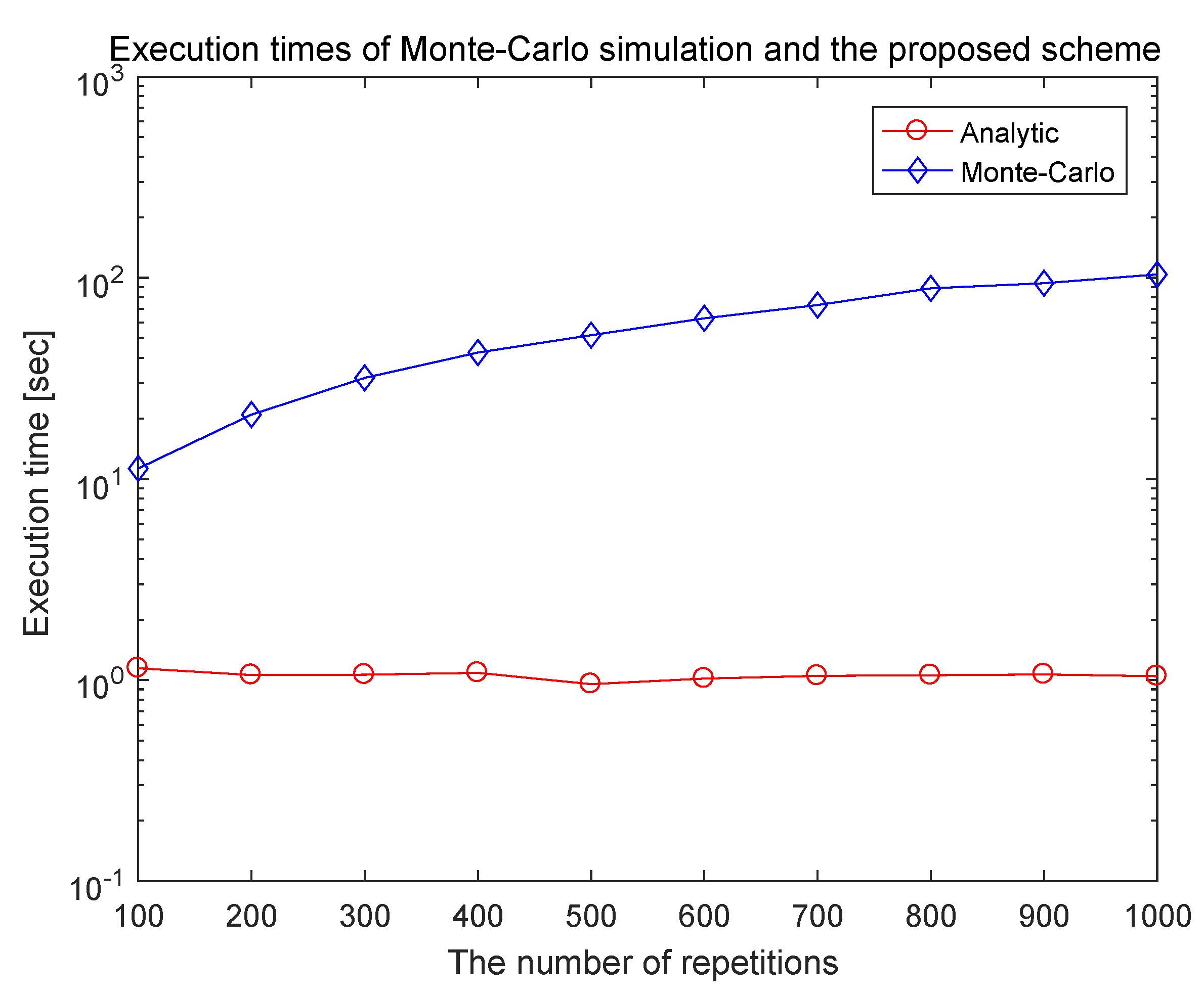
Instead, to quantify how computationally efficient the proposed algorithm is, execution time is obtained both for analytically derived MSE and for the Monte Carlo simulation-based MSE.

The number of incident signals is two, where two signals are incident from ${20}^{\circ }$ and ${40}^{\circ }$. The number of antenna elements is 10, and the number of snapshots is 1000. In getting the Monte Carlo simulation-based MSE, since the computational complexity is nearly proportional to the number of repetitions, the number of repetitions varies from 100 to 1000 in increments of 100.

Figure 5 shows how computationally efficient the proposed algorithm is. The execution times of the simulation-based MSEs and analytic MSEs are illustrated with respect to the number of repetitions. Note that the execution time for analytically derived MSE is essentially independent of the number of repetitions.

Figure 5. Comparing the execution times between Monte Carlo simulation-based MSEs and Analytic MSEs.

It is clearly shown in Figure 5 that execution time for the Monte Carlo simulation-based MSE is much greater than that for the analytically derived MSE even for the number of repetitions of 100. Figure 5 illustrates that getting analytically derived MSE is much less computationally intensive than getting Monte Carlo simulation based MSE, which justifies why the analytically derived MSEs should be employed for performance analysis.

6. Conclusions and Summary

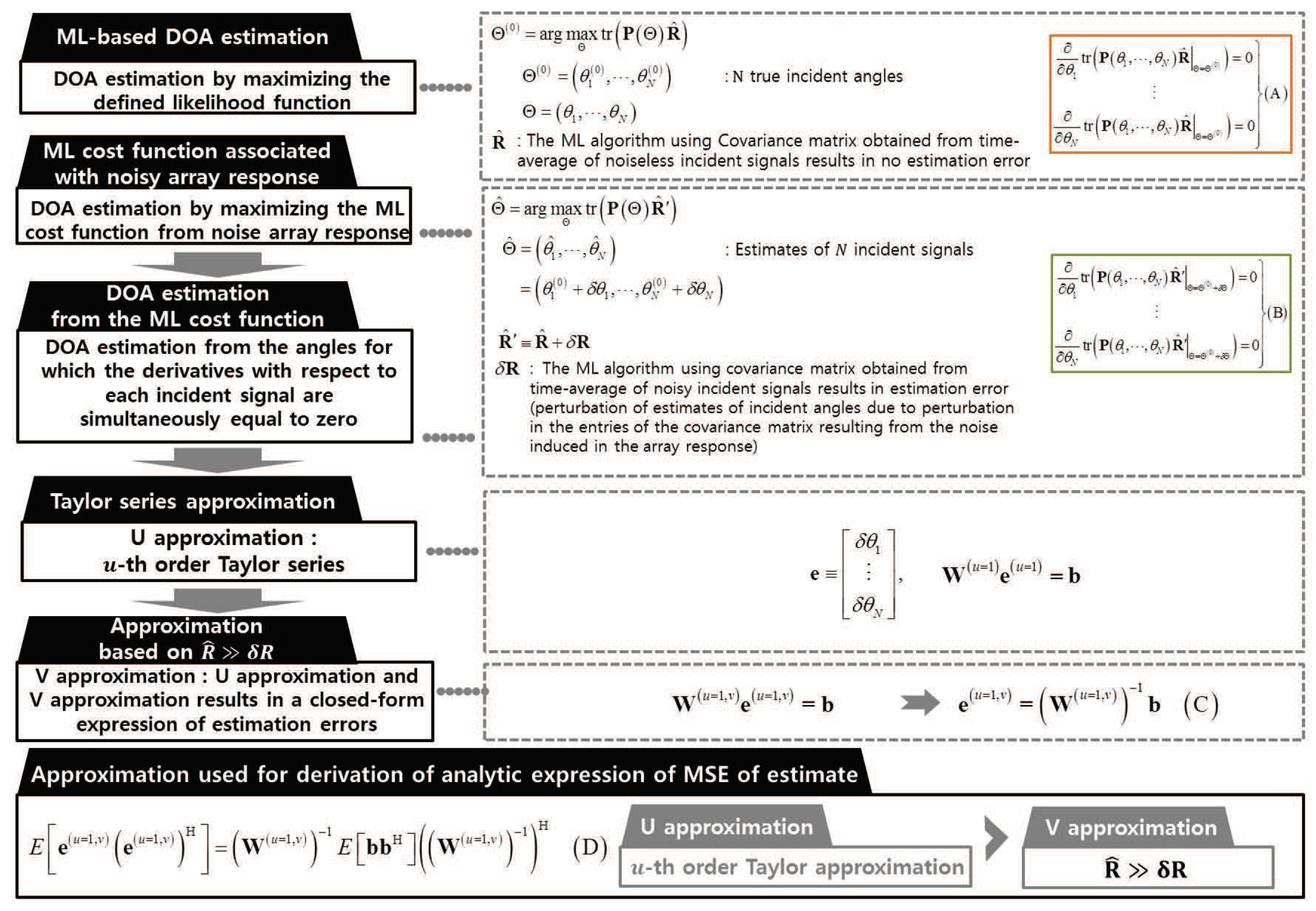
In Figure 6, the proposed algorithm is outlined. Note that Equations (A)–(D) in this section refer to Equations (A)–(D) in Figure 6, respectively. The constraints used for derivation of estimation errors are equations (A) and (B): equation (A) is valid since, in a noiseless environment, no estimation error occurs in the azimuth estimates. The estimation error due to an additive noise in noisy environment is formulated as equation (B).

Figure 6. Outline of the proposed performance analysis scheme.

To quantify the estimation error due to an additive noise, equations (A) and (B) and two approximations of U approximation and V approximation are used. Note that the covariance matrix in equation (A) and that in equation (B) are associated with noiseless response and noisy response, respectively. Applying the Taylor series approximation in equation (B) and using equation (A) in the approximated expression, the azimuth estimation error in equation (C) can be derived. To get an explicit expression of the MSE of the azimuth estimate, V approximation is applied, and the closed-form expression of the MSE of the estimate is obtained from equation (D).

To the best of our knowledge, no previous study used explicit equations (A) and (B) to derive the azimuth error in equation (C). One of the novelties of this paper is that the derivation is based on the observation that the azimuth error in the subscript in equation (B) can be analytically derived since equation (A) is true for noiseless covariance matrix.

In summary, applying U approximation to equation (B) and using the constraint in equation (A), the estimation error in equation (C) can be obtained. The MSE of the azimuth estimation error in equation (D) is obtained from equation (C) and V approximation. Note that, to get equation (D) from equation (C), the statistics of an additive noise should also be exploited.

Quantitative study on the estimation error for direction-of-arrival estimation in terms of standard deviation of an additive noise has been addressed in this paper.

In this paper, in case of estimating azimuths of multiple incident signals, the closed-form expression of the MSE of the DOA estimate for the ML algorithm has been derived by stepwise approximations. The type of antenna array is assumed as ULA. The closed-form of the MSE has been derived by using the Taylor series approximation which linearizes the nonlinear parts of the array vector and additional approximation based on the assumption that the estimation error is very small at high SNR. The closed-form of the MSE has been verified through numerical results. The closed-form of the MSE has been verified through numerical results. All of the stepwise approximated simulation results and the results obtained from the closed-form of the MSE show good agreement.

Although the formulation and the numerical results for two incident signals are presented in this paper, an extension to multiple incident signals is quite intuitively clear and straightforward.

In this paper, we rigorously derive how the MSE of the ML algorithm for direction-of-arrival can be expressed in terms of various parameters, which include the number of sensor elements, the number of incident signals, the number of snapshots, and the variance of additive noises on the antenna elements. Although, for convenience, the statistics of additive noise is assumed to be non-zero-mean Gaussian distributed, the derivation in the Appendices can be extended to the case where noise can be modeled as any other random variable as long as the moments of the random variable are analytically available.