Improved Active Interference Canceling Algorithms for Real-Time Protection of 2nd/3rd Level Facilities in Electronic Warfare Environment

Abstract

In an electronic warfare environment, important equipment or facilities of the friendlies are placed in protective facilities to protect against external Electronic Attacks (EA). No matter how well shielded the facility is, some external electromagnetic waves may penetrate through various paths such as power lines or fans, and the electromagnetic waves may be fatal to certain devices due to the structural resonance of the protective facilities. This paper introduced a real-time electromagnetic canceling technique that removes the resonance field inside the protection facility caused by the intended electronic attack from the enemy. The method makes it possible to cancel the process much faster than the conventional ones that have applied the Matrix Pencil Method (MPM). This is because the internal resonant field can be predicted in a closed-form under the assumption that the external electromagnetic wave is a complex exponential function. Longer exposure to Intended Electromagnetic Interference (IEMI) could be fatal for some devices. Therefore, it is imperative to attenuate the noise within a short time, and a method of reducing internal noise in real-time is beneficial for Electronic Protection (EP). The proposed method could be applied as a new technique to protect important protection facilities, rather than the more traditional method called wrapping using the Faraday cage effect.

1. Introduction

Electronic warfare is classified into an Electronic Attack (EA), Electronic Protection (EP), and Electronic Support (ES), and various researches are being conducted in each field [1,2]. While all areas are essential, their importance is increasing as the EPs must defend the electronic devices or facilities of friendlies from external attacks. The external attack is typically conducted using a radar jammer. An analysis of jamming effectiveness is also one of the most important studies of electronic warfare. There are several types of research on the calculations of jamming effectiveness [3,4]. Usually, electronic protection facilities are made of metal to defend against attacks from the outside, and they are defended using the Faraday cage effect. However, in reality, it is impossible to make a complete Faraday cage. This is because the power line for supplying the internal equipment is connected to the outside. Moreover, there are vents for internal ventilation [5,6]. Therefore, an electronic attack can affect the equipment in the electronic protection facilities, and various studies are being conducted to reduce them. To date, these facilities have added thicker barriers or shielding filters to meet the internal shielding standards [7]. High costs and space are required to make a shielding facility with a high shielding effect using this method.

Among the protection studies, there is a technique of canceling through directly analyzing the penetrated electromagnetic waves, rather than adding a shielding facility or using a shielding filter [8]. In this reference, the penetrated external electromagnetic wave is measured, and the signal is canceled by generating the same signal as the measured electromagnetic wave. The internally generated signal has an identical magnitude and frequency to the measured external electromagnetic waveform, but it is 180 degrees out of phase for eliminating internal interference. This principle is similar to the Active Noise Cancellation (ANC) method used in the acoustic field [9]. Since sound is also a wave, it can create a destructive interference phenomenon that can be used to make a noise-free zone at a particular location. To cancel in real-time, it requires a microphone and speaker, as well as an algorithm capable of processing a signal input through the microphone. The Finite Impulse Response (FIR) filter is mainly used, and various algorithms such as the Filtered-x Least Mean Square (FxLMS) and Filtered Error Least Mean Square (FELMS) exist in the algorithm applied to the filter [10,11].

Wavefield synthesis and wavefield analysis are based on wave equations using the Helmholtz–Kirchhoff integration without filters [12]. Each of these techniques uses the Helmholtz–Kirchhoff integration and appropriate boundary conditions to calculate the inner field or control the inner field. Several speakers and microphones are placed based on the quiet zone to apply this method. This method is called the massive multichannel ANC [13].

However, it is hard to apply this technique to electromagnetic waves. The most important reason is that the speed of the wave is different. The speed of waves used in electromagnetic waves is 300 million meters per second, like the speed of light, but the speed of waves applied to sound is 343 m per second, which is about 900,000 times different. In addition, the audible frequency uses a frequency of 20 Hz to 20 kHz, while the frequency range used in electronic warfare varies from the UHF band to the W band. It is challenging to produce precisely the same frequency to cancel this frequency band.

Additional analysis algorithms are needed to solve this problem, after the first cancellation, since only a slight frequency difference between the external and internally generated waveform can cause amplification rather than cancellation of the internal field. Previous studies have used the matrix pencil method to predict these frequency differences [14]. The MPM can predict the frequency difference very accurately but requires an adequate number of samples to find the frequency. The time required to collect this sample can be fatal to the protective equipment in some cases.

The real-time noise reduction technique presented in this paper can estimate the frequency difference much faster than the conventional methods under the assumption that the externally incident electromagnetic waves are complex sinusoids. Theoretically, it can be obtained with only one sampling information, but the accuracy is much lower in noisy situations. This problem was overcome by increasing the sampling time, while accurately estimating the frequency difference through much less sampling than the conventional methods.

The rest of the paper is organized in the following order: In Section 2, the Intended Electromagnetic Interference (IEMI) produced by EA is coupled into the protection facility, and the conventional method of removing the penetrated electromagnetic wave using MPM is introduced. Afterward, detailed mathematical development of the algorithm that can reduce the interference in real-time is presented in Section 3, and in Section 4, the calculated results are compared. Finally, the paper concludes with discussions and conclusions.

2. Radiated Coupling and Active Noise Cancellation

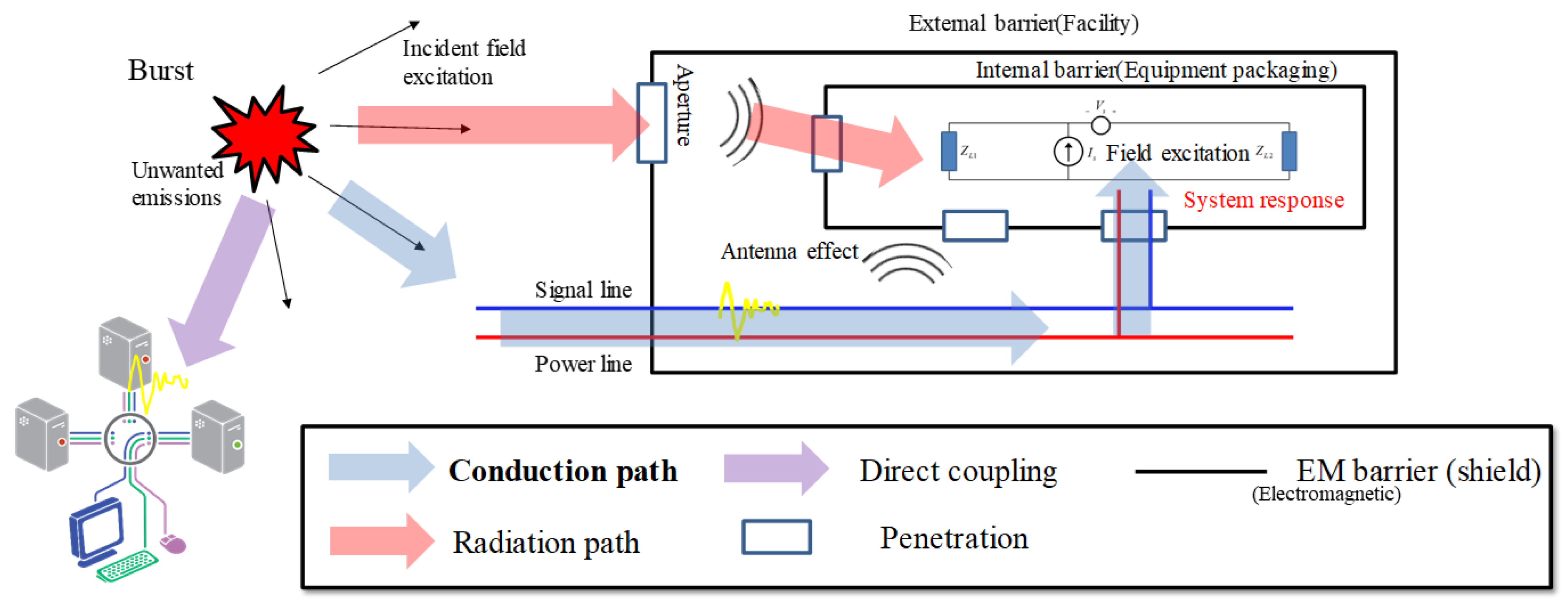
In an electronic warfare environment, the externally intended attack reaches a major friendly facility through the atmosphere. A High-altitude Electromagnetic Pulse (HEMP) or jammer attacks occur at relatively long distances (hundreds of kilometers), and the victims are attacked using plane waves. This attack has a wide frequency characteristic, the strongest of which is at the resonant frequency, which is most affected by the size of the structure of the protective installation. Figure 1 shows the various coupling paths in the electronic warfare environment.

This attack affects friendly protection facilities, mainly metal resonators, and the size of the protection facilities determines the resonant frequency. In general, the resonance frequency of an ideal resonator without an aperture is expressed by Equation (1).

$$f_r^{mnp}=\frac{1}{2\pi \sqrt{\mu \epsilon }}\sqrt{{\left(\frac{m\pi }{a}\right)}^2+{\left(\frac{n\pi }{b}\right)}^2+{\left(\frac{p\pi }{c}\right)}^2}$$

(1)

where μ is the permeability, ε is the permittivity, a is the width of the resonator, b is the length, and c is the height. m is a mode number for the resonator transverse axis, n is a mode number for the longitudinal axis, and p is a mode number for the height axis. This mode number is the Transverse Electric (TE) mode where m and n are integers starting from zero, and p is an integer starting from one. In the Transverse Magnetic (TM) mode, m and n are integers starting at one, and p is an integer starting at zero.

When apertures exist for this resonator for various reasons, the quality factor Q is determined by the aperture size, which causes a slight shift in the resonant frequency. In the absence of an aperture, one of the most critical parameters of the resonator, Q, is defined as

$$Q\equiv \omega \frac{W_t}{P_d}=\omega \frac{W_e+W_m}{P_d}$$

(2)

where ω is the angular frequency, W_t is the stored energy inside the cavity, P_d is the dissipated power, W_e is energy due to the electric field, and W_m is energy due to the magnetic field. Total dissipated power is found by adding power dissipated in each of the six walls of the cavity. The dissipated power on the top wall is similar to the bottom, and power on the right wall is like the left. Meanwhile, dissipated power on the back is the same as that on the front. Thus, the total dissipated power can be written by

$$P_d=\frac{R_s}{2}\left\{2{\displaystyle {\iint }_{bottom}{J}_b\cdot J_b^{*}ds}+2{\displaystyle {\iint }_{left}{J}_l\cdot J_l^{*}ds}+2{\displaystyle {\iint }_{front}{J}_f\cdot J_f^{*}ds}\right\}.$$

(3)

where R_s is the surface resistance and J_b, J_l, and J_f are the current density of bottom, left, and front wall, respectively.

If there is an aperture in the resonator, the resulting loss occurs, and the overall Q value is determined through four mechanisms [15]. The first is caused by the current flowing through the inner wall of the resonator. The internal absorber generates the second. The third is caused by antenna loss, and the last is caused by aperture loss. The total Q through these four mechanisms is determined by

$$\frac{1}{Q}=\frac{1}{Q_{surf}}+\frac{1}{Q_{TCS}}+\frac{1}{Q_{ant}}+\frac{1}{Q_{ACS}}$$

(4)

where Q_surf is the Q value determined by the wall surface, Q_TCS is the abbreviation for the Transmission Cross Section (TCS), and is determined while transmitting internally. Q_ant is the Q value determined by the antenna loss, and Q_ACS is determined by the abbreviation for the Aperture Cross Section (ACS). As you can see from the above Equation, the smallest Q value has the most significant effect on the total Q value.

Protection facilities are classified in stages or levels according to their location and purpose. The most directly affected outermost facilities, such as buildings or HEMP protection facilities, are classified as 1st level barriers, and their physical size ranges from a few meters to several tens of meters. There are enclosures or small screen rooms enclosing equipment inside the protection facility. These facilities are classified into 2nd and 3rd level barriers. These additional barriers are as small as a few centimeters to tens of centimeters [16,17,18]. In this paper, the 2nd ~ 3rd level barrier was studied.

The acoustics field has been studied for a long time to cancel external noise. This technique, called ANC, detects external noise sources through speakers and cancels them with a microphone. For this purpose, the Finite Impulse Response (FIR) filter is used, and the most commonly used algorithm is the FxLMS technique. Recently, a canceling technique using the Genetic Algorithm (GA), one of the optimization techniques, was studied [10].

A technique for attenuating internally generated electromagnetic interference using the principle of the ANC technique was introduced in the paper [8]. External interference signals, expressed as sinusoids, are measured by sensors inside the shielding facility. At this time, we measure the amplitude, frequency, and phase of the external signal. Based on this measured information, it internally generates a signal with the same amplitude and frequency, but it is 180 degrees out of phase with the active source. At this time, the internally observed signal follows this formula for the sinusoidal signal.

$$S_{obv}\left(t\right)=\frac{{\left(A_I\cos \left(2\pi ft+\varphi \right)+A_{ac}\cos \left(2\pi f^{\prime }t+{\varphi }^{\prime }\left(t\right)\right)\right)}^2}{Z}$$

(5)

where A_I is the amplitude of the IEMI, f is the frequency of the IEMI, and ϕ is the phase of the IEMI. A_ac is the amplitude of the generated signal, f′ is the frequency of the generated signal, ϕ′ is the phase of the generated signal. At this time, for the internally measured signal to be zero, the amplitude and frequency must be the same, and the phase must be different by π. To satisfy this condition,

$$A_I=A_{ac}, f=f^{\prime }, \left|{\varphi }^{\prime }-\varphi \right|=\pi$$

(6)

This formula must be satisfied.

It is relatively easy at this time to make the amplitudes equal or to make the phase difference 180 degrees, but it is challenging to make the frequency accurate. In the acoustics field, the ANC technique is used to cancel the audible frequencies, which are in the range of about 20 Hz to 20 kHz. It is relatively easy to measure and regenerate this frequency. However, the frequency applied to electronic warfare is several GHz, and it is impossible to make the same frequency for these attacks. 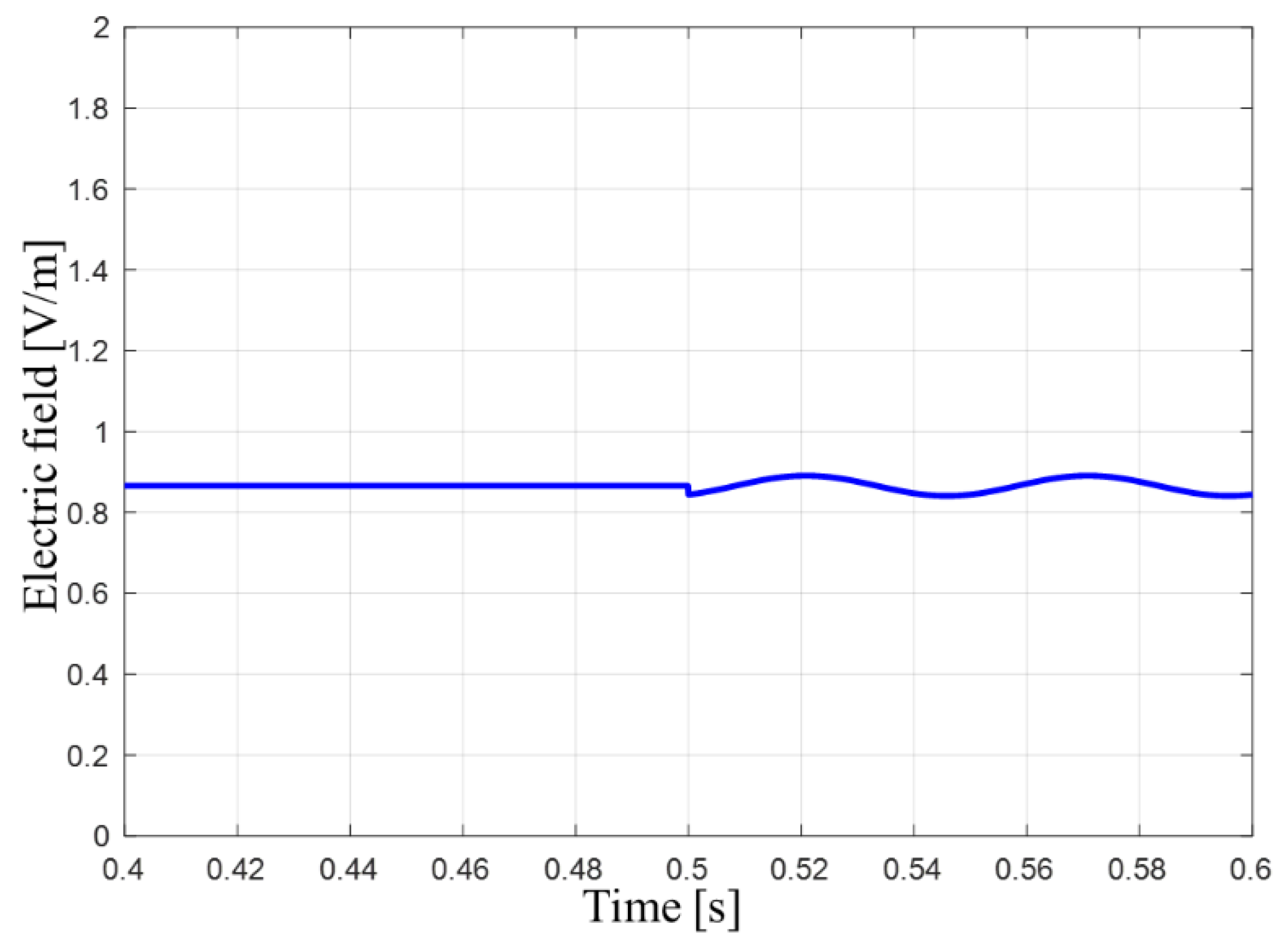Figure 2 below shows that the internal field is amplified rather than canceled when there is a difference of only 20 Hz internally for an external attack with a frequency of 2 GHz.

MPM is used to solve this amplification. First, assuming that the same frequency cannot be generated, create a small signal equal to 2.5% of IEMI on active power. Then, the synthesized signal is analyzed once again. If there is a frequency difference of about 20Hz, as in the above example, the internal signal is not canceled. The IEMI and the internal active signal combine to produce a 20 Hz sine wave. At this time, this signal is analyzed by MPM. MPM is a technique that performs extrapolation based on given data and is applied to a sinusoidal signal very accurately. This method has been verified through many papers. 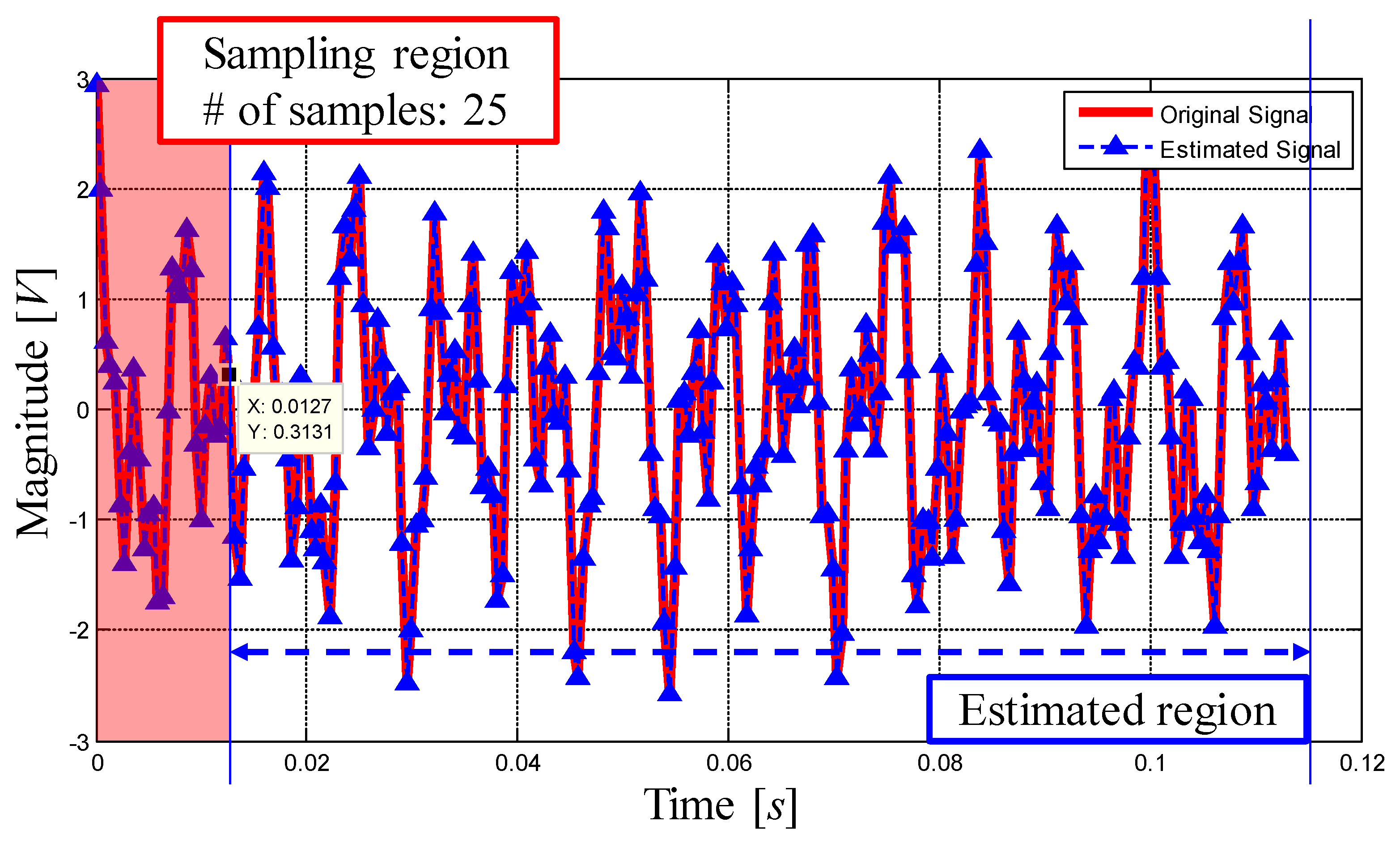Figure 3 shows the results of estimating randomly generated signals using MPM. The red line represented the original signal and generated a signal with a total of 250 points. At this time, the estimation was performed using only about 1/10 of the signals. The red area shown in the Figure 3 is the sampling area, and the area indicated by the blue line is the estimated area. The rest is correctly estimated for the original signal using only a few samples from the beginning.

The internal signals can be canceled accurately using this technique by analyzing the mixed signal of the IEMI and active signals. The active cancellation algorithm using MPM can be summarized as follows:

• Step 1. Measure the amplitude, frequency, phase of the IEMI, and apply small active power.
• Step 2. Measure the sensor power signal S_obv of IEMI at the position to cancel.
• Step 3. Use MPM to calculate the magnitude, phase, and frequency difference of the mixed-signal.
• Step 4. Apply the value calculated in step 3 to the internal active power source
• Step 5. Determine whether the internal electromagnetic field is reduced below the standard value. If the standard value is not satisfied, then repeat from Step 2.

Figure 4 shows the result of analyzing the signal using the MPM and canceling the internal field using the result.

This method has the advantage of canceling the internal IEMI by analyzing the signal through the MPM, but there is the time taken to analyze the MPM, that is, the “blind time.” During this time, the friendly equipment is unprotected from external attacks, and this attack can even be amplified. Therefore, reducing this time is very important for electronic protection. To reduce this time, the time to analyze the signal must be reduced, and a faster algorithm than the conventional MPM is required.

3. Real-Time Interference Cancellation

To reduce the “blind time,” a weakness of MPM-based active noise cancellation, the time to analyze the signal must be reduced. MPM uses some of the sampled information to make various calculations. Various calculations are required, such as performing matrix operations or determining singular values, which require some time, that is, a certain number of samplings. To minimize this sampling, the technique presented in this paper was used. This method assumes that the amplitude, phase, and sampling time step of the initial IEMI are known, and the externally incident IEMI is assumed to be a complex exponential wave. At this time, the complex sinusoidal signal can be expressed as the following Equation.

$$y\left(t\right)=A_I\exp \left(j\left(2\pi f_{I}t+{\varphi }_I\right)\right)$$

(7)

Next, the signals produced by the internal active power supply are summed, which has a frequency difference of Δf compared to the original signal. This is expressed as the formula below.

$$y_s\left(t\right)=A_I\exp \left(2\pi f_{I}t+{\varphi }_I\right)+A_{ac}\exp \left(2\pi \left(f_I+\mathsf{\Delta }f\right)t+{\varphi }^{\prime }\right)$$

(8)

Figure 5 shows the combined signal when A_ac is 2.5% of A_I and ϕ_I = 30°.

The time axis was sampled at 0.001 s, and the active signal was applied at 0.5 s. From this time, it was confirmed that there was no cancellation due to the frequency difference, and it was fluctuating slightly. Since the fundamental frequency was very high compared to the sampling frequency, it could be seen that the section before 0.5 s, where only IEMI, exists looked like DC. Therefore, the sampled signal for the section after 0.5 s is shown as a function of Δf. This is expressed as the following formula.

$$y_{sp}\left(t\right)=A_{ac}\exp \left(j\left(2\pi \mathsf{\Delta }ft+\varphi \right)\right)$$

(9)

For this signal, the measured value at t₁ s and the measured value at t₂ s are compared.

$$y_{sp}\left(t_1\right)=A_{ac}\exp \left(j\left(2\pi \mathsf{\Delta }f{t}_1+\varphi \right)\right)$$

(10)

$$y_{sp}\left(t_2\right)=A_{ac}\exp \left(j\left(2\pi \mathsf{\Delta }f{t}_2+\varphi \right)\right)$$

(11)

At this time, t₂ is equal to t₁ + Δt,

$$y_{sp}\left(t_2\right)=A_{ac}\exp \left(j\left(2\pi \mathsf{\Delta }f\left(t_1+\mathsf{\Delta }t\right)+\varphi \right)\right)$$

(12)

$$y_{sp}\left(t_2\right)=A_{ac}\exp \left(j\left(2\pi \mathsf{\Delta }f{t}_1+2\pi \mathsf{\Delta }f\mathsf{\Delta }t+\varphi \right)\right).$$

(13)

Here, use Euler’s formula to expand the measurement at t₂ s,

$$y_{sp}\left(t_2\right)=A_{ac}\left[\cos \left(\left\{2\pi \mathsf{\Delta }f{t}_1+\varphi \right\}+2\pi \mathsf{\Delta }f\mathsf{\Delta }t\right)+j\sin \left(\left\{2\pi \mathsf{\Delta }f{t}_1+\varphi \right\}+2\pi \mathsf{\Delta }f\mathsf{\Delta }t\right)\right].$$

(14)

To simplify the expression, replace 2πΔft₁ + ϕ = A, 2πΔfΔt = B, and then apply the trigonometric formula.

$$y_{sp}\left(t_2\right)=A_{ac}\left[\cos A\cos B-\sin A\sin B+j\left(\sin A\cos B+\cos A\sin B\right)\right]$$

(15)

It is assumed here that the sampling time, Δt, is much shorter than t₁, and frequency difference, Δf, is also less than 100. This also assumes that the generated frequency from the active source is close to the externally measured frequency. From this assumption, ΔfΔt is close to zero. That means B has a very small value. The series expansion of the sine and cosine functions is shown below.

$$\begin{array}{l}sps,\mathsf{\Delta }t\ll 1<t_1, \mathsf{\Delta }f<100\to \mathsf{\Delta }f\mathsf{\Delta }t\approx 0\\ \Rightarrow \sin x=x-\frac{x^3}{6}+\cdots ,\hspace{1em}\cos x=1-\frac{x^2}{2}+\frac{x^4}{24}-\cdots \end{array}$$

(16)

ΔfΔt is assumed to be close to zero. As mentioned earlier, the substituted B value above also comes close to zero. This assumption allows approximating the sine function up to the first term and the cosine function up to the second term. The signal sampled at t₂ can be arranged using this assumption as follows.

$$\begin{array}{cc}\hfill y_{sp}\left(t_2\right)& =\cos A\left(1-\frac{B^2}{2}\right)-B\sin A+j\left(\sin A\left(1-\frac{B^2}{2}\right)+B\cos A\right)\hfill \\ & =\left(\cos A+j\sin A\right)-\frac{B^2}{2}\cos A-B\sin A+j\left(-\frac{B^2}{2}\sin A+B\cos A\right)\hfill \\ & =\left(\cos A+j\sin A\right)+jB\left(\cos A+j\sin A\right)-\frac{B^2}{2}\left(\cos A+j\sin A\right)\hfill \end{array}$$

(17)

The above Equation is a modification of the time sampled at t₂ s, and in this modified Equation, the function of the time sampled at t₁ can be found. Applying this function is equivalent to Equation (18).

$$y_{sp}\left(t_2\right)=y_{sp}\left(t_1\right)+jB{y}_{sp}\left(t_1\right)-\frac{B^2}{2}{y}_{sp}\left(t_1\right)$$

(18)

The purpose of this method is to find the frequency difference Δf from IEMI, so to sum up the above Equations for B, the expressions are arranged in perfect squares form. Equation (19) is the process of arranging a perfect square expression.

$$\begin{array}{cc}\hfill y_{sp}\left(t_2\right)-\frac{1}{2}{y}_{sp}\left(t_1\right)& =\frac{1}{2}{y}_{sp}\left(t_1\right)+jB{y}_{sp}\left(t_1\right)-\frac{B^2}{2}{y}_{sp}\left(t_1\right)\hfill \\ & =\frac{1}{2}{y}_{sp}\left(t_1\right)\left(1+j2B-B^2\right)\hfill \\ & =\frac{1}{2}{y}_{sp}\left(t_1\right){\left(1-jB\right)}^2\hfill \end{array}$$

(19)

After arranging this for B, Δf is obtained by substituting 2πΔfΔt into B in Equation (19).

$$\mathsf{\Delta }f=\frac{1}{j2\pi \mathsf{\Delta }t}\left(1-\sqrt{2\frac{y_{sp}\left(t_2\right)}{y_{sp}\left(t_1\right)}-1}\right)$$

(20)

The above Equation can be used to estimate the difference between two frequencies using the sampled signal at t₁ and t₂ time. Theoretically, the frequency difference can be predicted using only two samplings.

However, in the presence of noise, the accuracy is very low. Signals are sampled for a specific period to overcome this problem, and then averaging is used to estimate frequency difference. This is similar to the averaging or average filter technique used in many measurement instruments and shows good agreement when white Gaussian noise is presented. By applying this method to the Equation for estimating the frequency difference, it can be expressed as Equation (21).

$$\mathsf{\Delta }f=\frac{1}{N}{\displaystyle \sum _{k=1}^N\mathsf{\Delta }{f}_k}, \mathsf{\Delta }{f}_k=\frac{1}{j2\pi \mathsf{\Delta }t}\left(1-\sqrt{2\frac{y_{sp}\left(t_{k+1}\right)}{y_{sp}\left(t_k\right)}-1}\right)$$

(21)

Applying this averaging estimation method to the MPM calculation, part of the active cancellation algorithm, can reduce the overall simulation time. The newly proposed algorithm is shown below in Figure 6.

4. Simulation Result

In this section, the real-time interference cancellation technique described above is applied to analyze in the noiseless and the presence of white Gaussian noise. In the conventional method using the MPM, when determining the singular value, it is determined by the user’s discretion. When there are N singular values generated among MPM internal operations, only σ_c values satisfying the following formula are selected based on the largest value σ_max.

$$\frac{{\sigma }_c}{{\sigma }_{\max }}\ge {10}^{-p}$$

(22)

where p is the number of significant decimal digits in the data, as an example, if the simulation results are accurate up to 3 significant digits, then the singular values which have less than 0.001 compared to the largest singular value are noise singular values. They should not be used in the reconstruction of the data. Therefore, based on this p value, it is determined how many signals are combined. However, to simplify the calculation of MPM, the simulation was performed, assuming that there were only two signals to analyze.

Figure 7 shows the result of estimating the signal using MPM under noiseless conditions. At this time, the signal formula and conditions are shown in Equation (23) and

Table 1. Variables used in Equation (23).

Category	Symbol	Value	Unit
Magnitude	AI	1	V/m
Phase	ϕ	30	°
Frequency	f	2	GHz
Frequency difference	Δf	20	Hz

.

$$y\left(t\right)=A_I\cos \left(2\pi ft+\varphi \right)+A_{ac}\cos \left(2\pi \left(f+\mathsf{\Delta }f\right)t+{\varphi }^{\prime }\right)$$

(23)

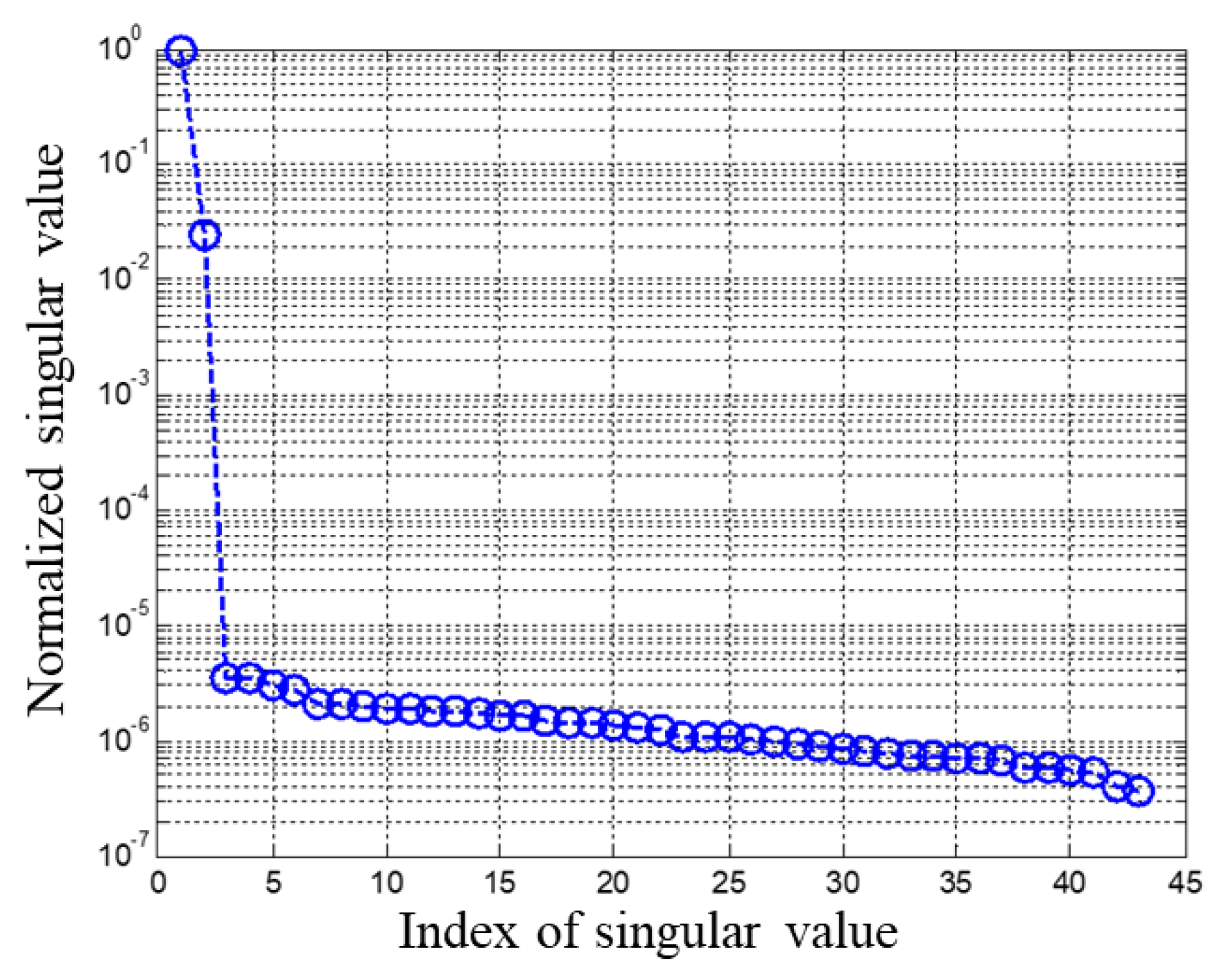
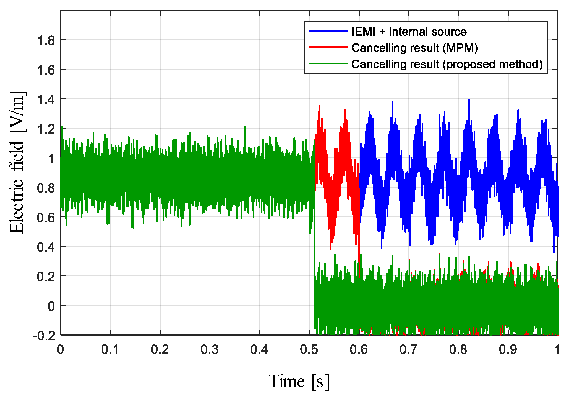
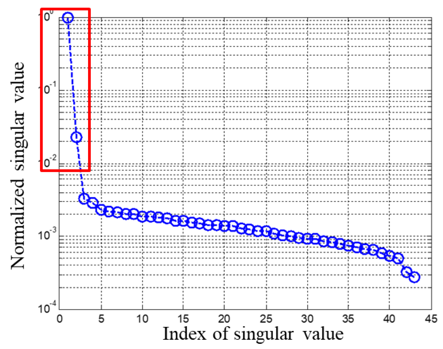
The blue line in the Figure 7 is the result of the combination of the interference signal and the internal AC signal at 0.5 s after the external IEMI is incident, and before the MPM is applied. In the MPM method, the cancellation was completed after a total of 100 ms of time, and the result was a red line. At this time, if the number of sampling was reduced to reduce the blind time, accurate estimation was not made, and the signal was amplified after cancellation. When applying the MPM, singular values are shown in Figure 8. As mentioned above, only two of them were selected.

On the other hand, in the case of simulations using the proposed method, accurate cancellation could be performed through a single sampling immediately after sensing an external signal. This is shown in Figure 9. The process requires 1ms of computation time on the time axis and can be calculated 100 times faster than with conventional methods.

In noisy situations, accurate estimation is not possible with only one step. Figure 10 is the same situation as before, but with the white Gaussian noise applied. At this time, the signal formula and conditions are shown in Equation (24) and

Table 2. Variables used in Equation (24).

Category	Symbol	Value	Unit
Magnitude	AI	1	V/m
Phase	ϕ	30	°
Frequency	f	2	GHz
Frequency difference	Δf	20	Hz
Signal to noise ratio	SNR	20	dB

.

$$y\left(t\right)=A_I\cos \left(2\pi ft+\varphi \right)+A_{ac}\cos \left(2\pi \left(f+\mathsf{\Delta }f\right)t+{\varphi }^{\prime }\right)$$

(24)

Even when the Signal to Noise Ratio (SNR) is 20 dB, Figure 10 shows that the MPM can be applied to cancel the system accurately. At this point, the singular values, as demonstrated in Figure 11, are higher than before due to white Gaussian noise. If you set p = 3, it is impossible to make an accurate estimate when using MPM. This result is because too many singular values exceed the reference value, 10⁻³, which determines that there are approximately 25 signals. On the other hand, even in this situation, the proposed method accurately predicts the frequency difference using only 50 sampled data with the averaging. The result is 5 ms on the time axis and provides a 20× time efficiency gain over conventional methods that require 100 ms of computation time.

In the previous paper mentioned before [8], the experiments were conducted using the vehicle model. In this experiment, the scaled-down model was used, and the canceling was carried out using a magnetic loop feeder inside the vehicle engine room. It took 155~188 ms for MPM analysis and cancellation, and 400~500 ms in total. The MPM operation relies on the performance of the computer’s Central Processing Unit (CPU) because it takes the measured value from the power meter to the user’s computer and processes it. In this paper, the vehicle engine room part was simulated similarly to the above situation. The size of the resonator and input path of IEMI is as below in

Table 3. The size of the vehicle engine room part and the information of IEMI.

Category	Size	Unit
Cavity	200 × 150 × 150	mm
Aperture	50 × 70 × 2	mm
IEMI direction	−z	Vector
Frequency range	1~3	GHz

.

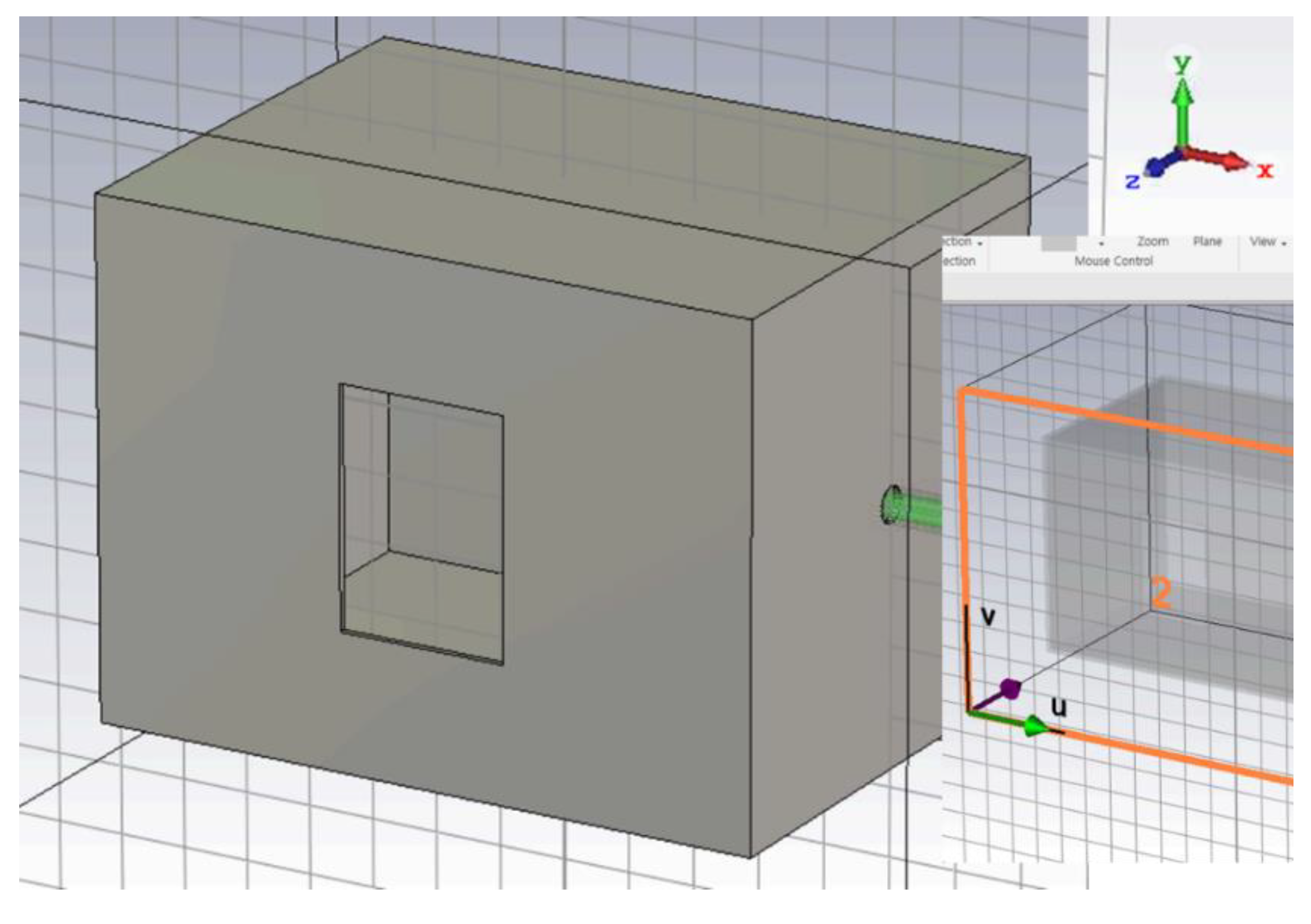
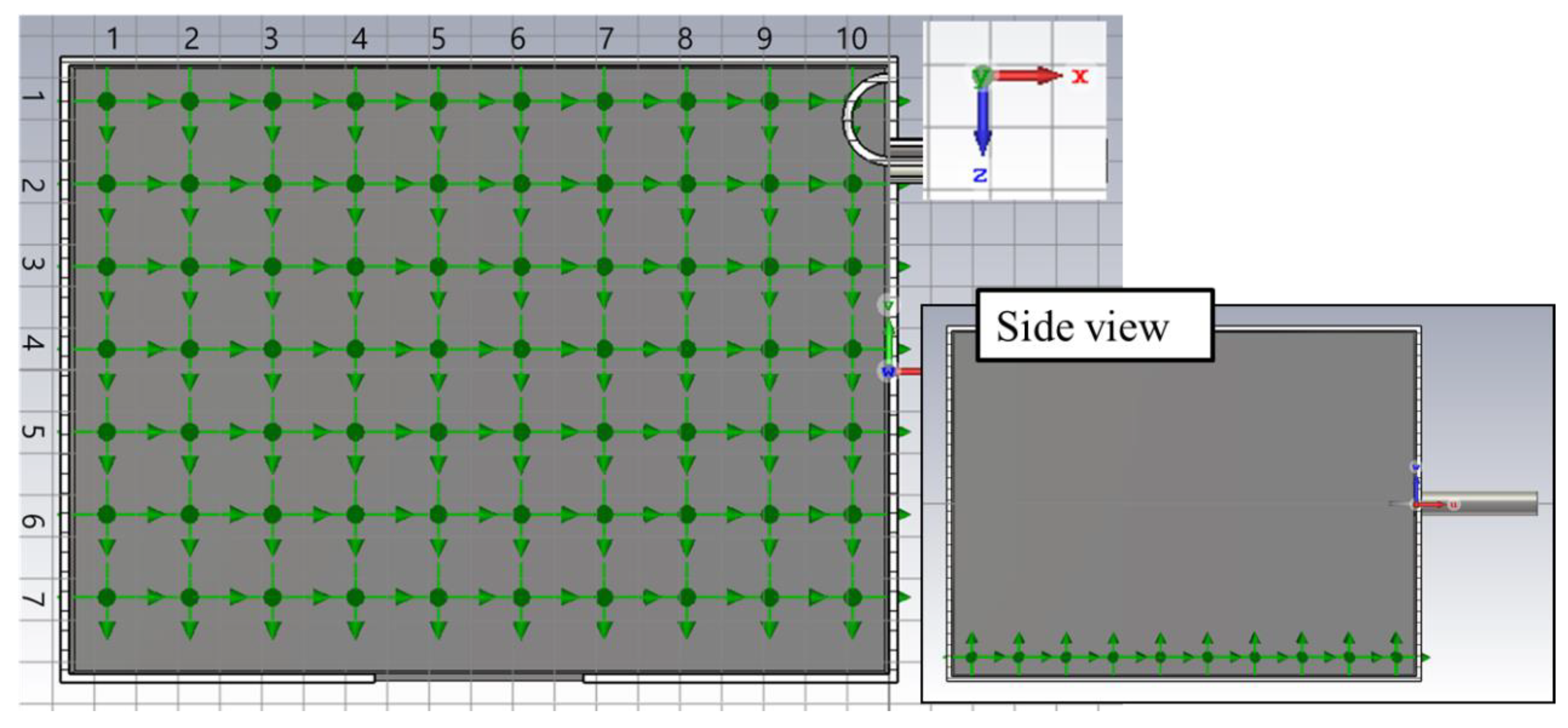
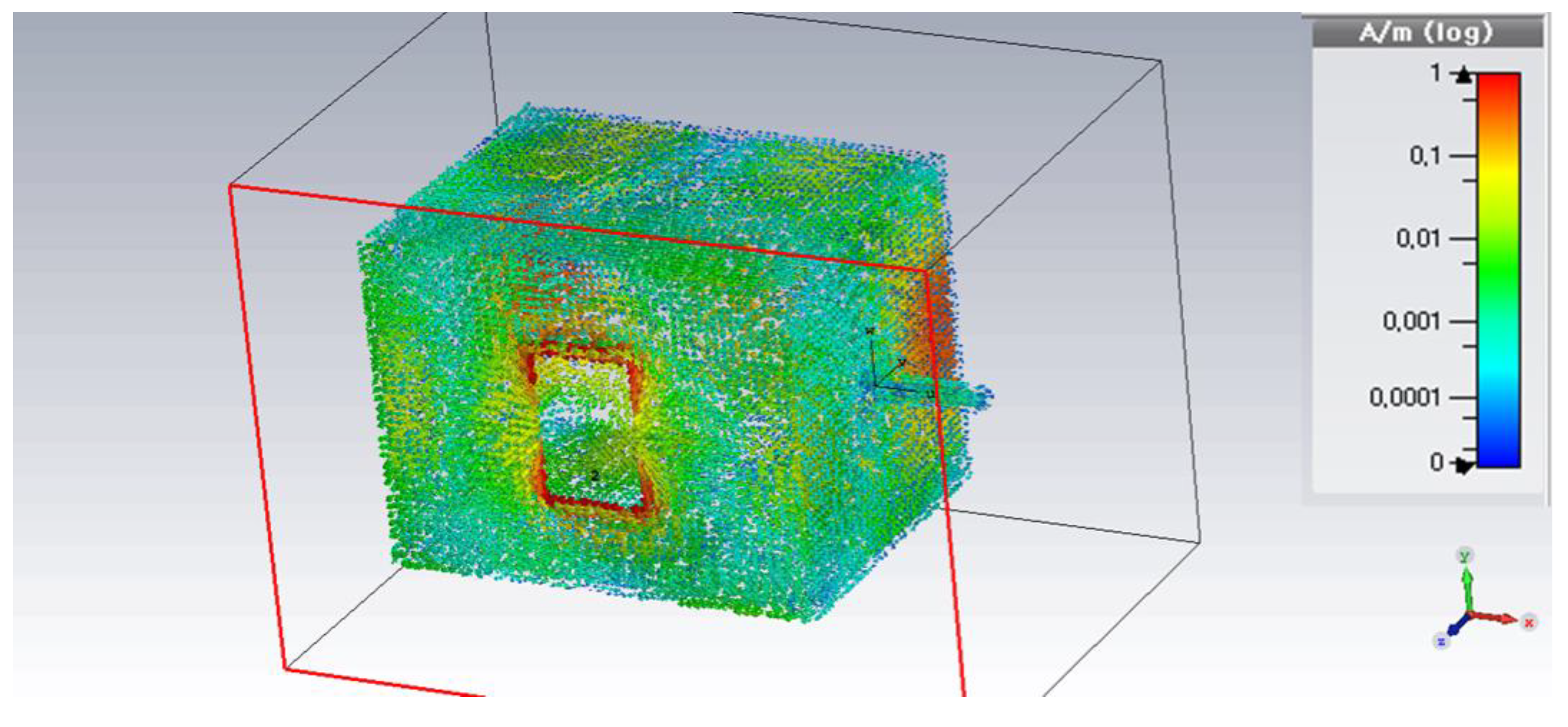
For effective internal field cancellation, the feeder should be installed where the surface current is most dense. The equipment is usually installed at the bottom of the protection facilities. Thus, the field is observed by installing sensors on the bottom of the cavity. A total of 70 probes were installed, i.e., 10 horizontally and 7 vertically, each 20 mm apart, 8 mm from the bottom. The figures below (Figure 12, Figure 13 and Figure 14) show the shape of the cavity, the arrangement of the antennas, and the current distribution when the IEMI is incident from the front.

In the resonator of this size, the resonance frequency is about 1.25 GHz with the smallest value in the 101 mode. The resonance frequencies for several modes in the resonator are shown in

Table 4. Resonance frequency depending on the mode of this resonator.

m	n	p	Frequency [GHz]
1	0	1	1.249
0	1	1	1.413
1	1	1	1.599
2	0	1	1.801
2	1	1	2.060
2	2	1	2.690
1	0	2	2.134
0	1	2	2.234
2	0	2	2.498

.

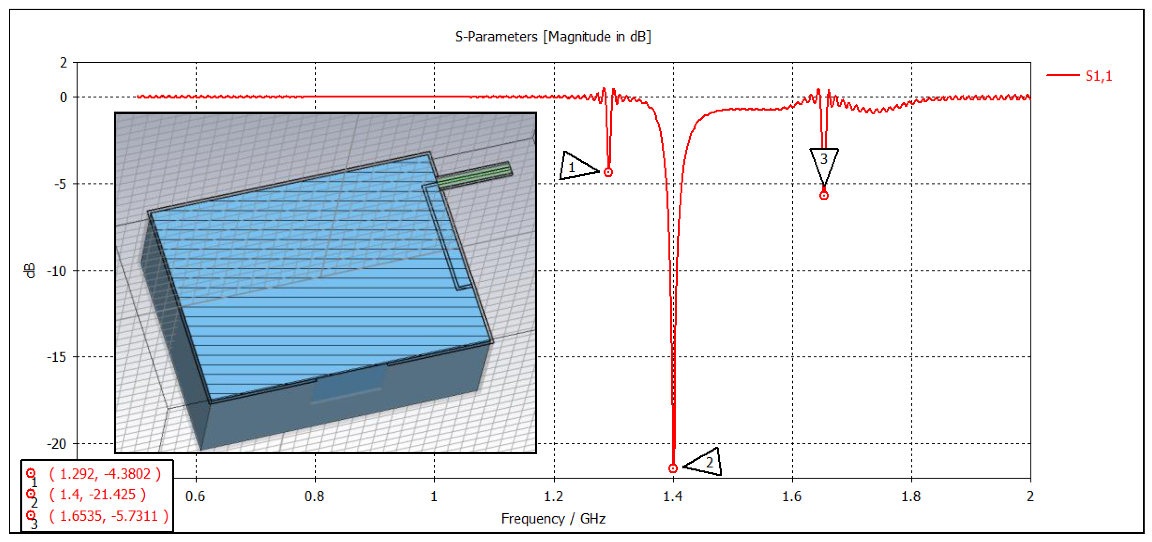
In this study, the target frequency was 1.414 GHz and canceled the resonance occurring at that frequency. The feeding structure for canceling the internal field was made using the loop type magnetic field feeder of the rectangular shape and installed based on the place where the current is most concentrated. Figure 15 shows the feeder shape and its S-parameters.

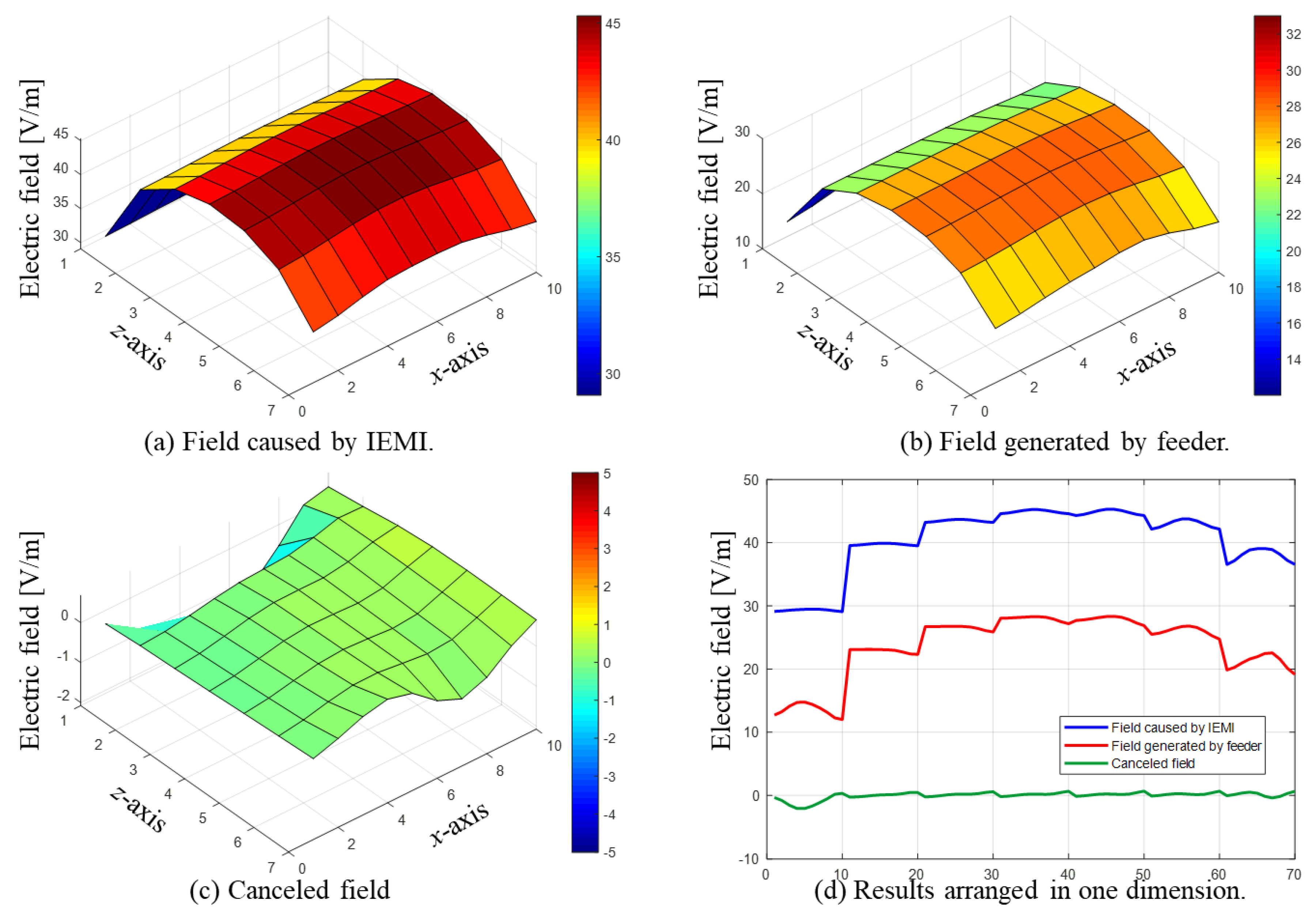
The field when the IEMI enters from the outside was measured by 70 probes installed earlier. Figure 16a shows the result of plotting the field on the bottom at a specific frequency by post-processing the result. In the same situation, the feeder generates an estimated canceling signal using a real-time reduction technique. The result of plotting this signal in the same position as before is also shown in Figure 16b.

The field canceled by the generated signal estimated by the proposed technique is shown in Figure 16c. After arranging the addresses given to the electric field probes in a row, the results of the comparison in a one-dimensional graph were added to Figure 16d.

5. Discussion and Conclusions

In an electronic warfare environment, an enemy’s intended attack harms the equipment pf friendly forces. Protective facilities exist to defend these attacks, and even if these protective facilities exist, infiltration into friendly equipment also occurs. In this paper, the real-time active interference cancellation algorithm was proposed for external intended electromagnetic interference penetrating from the 2nd level to 3rd level. Many articles and reports of the conventional approaches for HEMP protection have been suggested as a sort of primitive method of direct shielding through some special materials or modified plant structures. However, by installing a small feeder in the resonator or protective facility, this new innovative idea might provide a comfort electromagnetic environment inside the facilities. In addition, the proposed algorithm can be calculated from 20 to 100 times faster than the existing research using the MPM, and it is confirmed that the electric field is canceled inside the resonator using the Computer Simulation Technology (CST) microwave studio tool. In this work, the external electromagnetic waveform was canceled by focusing on one of several modes that occur in the resonator. However, in the future, the multi-feeder technique to apply the canceling method to various modes and the optimized feeder design study that can cancel the target frequency more efficiently may be used to obtain better results.