An Adaptive Approach for Multi-National Vehicle License Plate Recognition Using Multi-Level Deep Features and Foreground Polarity Detection Model


Abstract
Featured Application
Abstract
1. Introduction
2. Related Work
3. Proposed Methodology
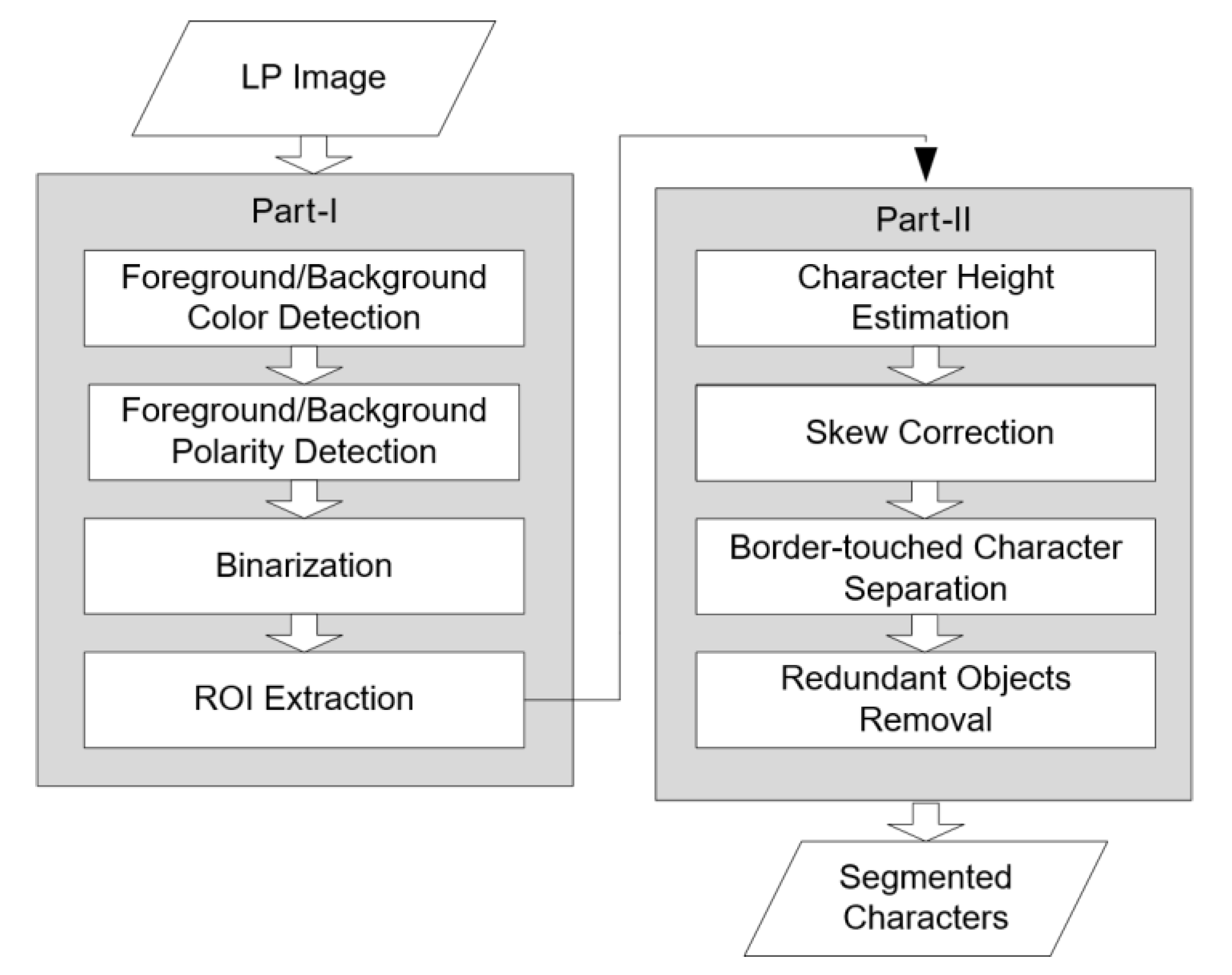
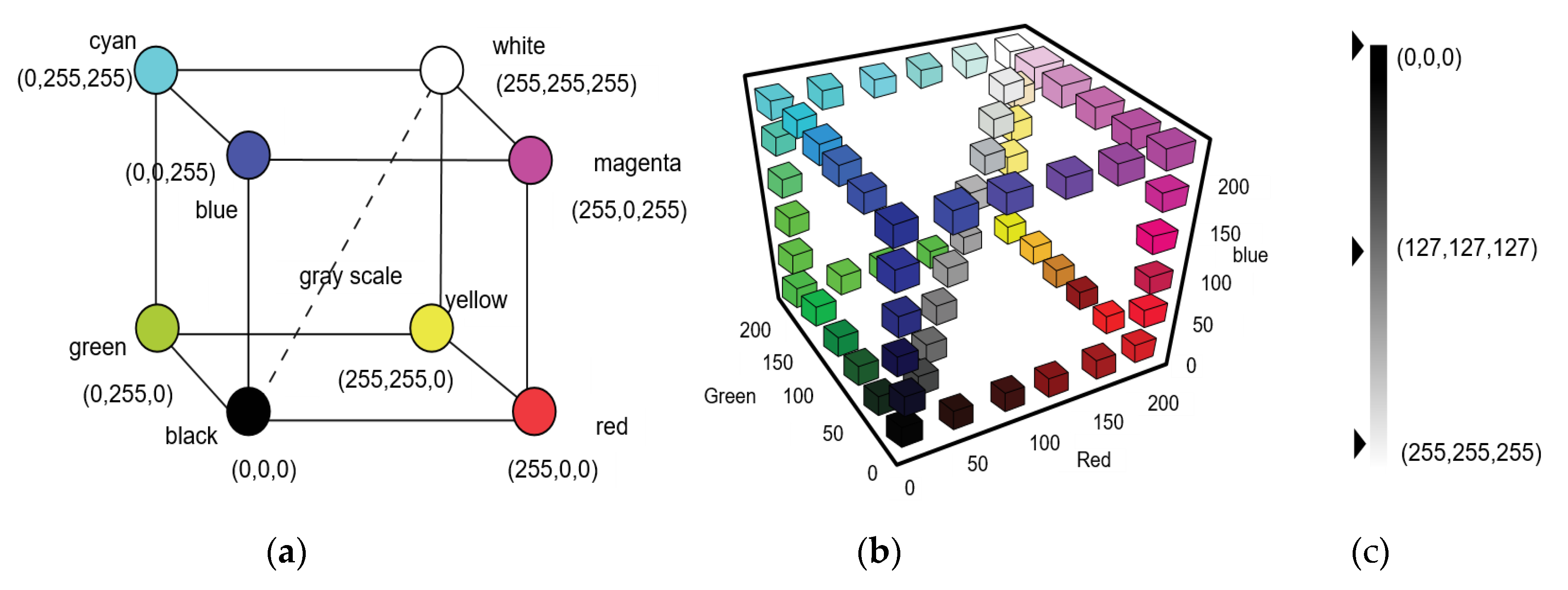
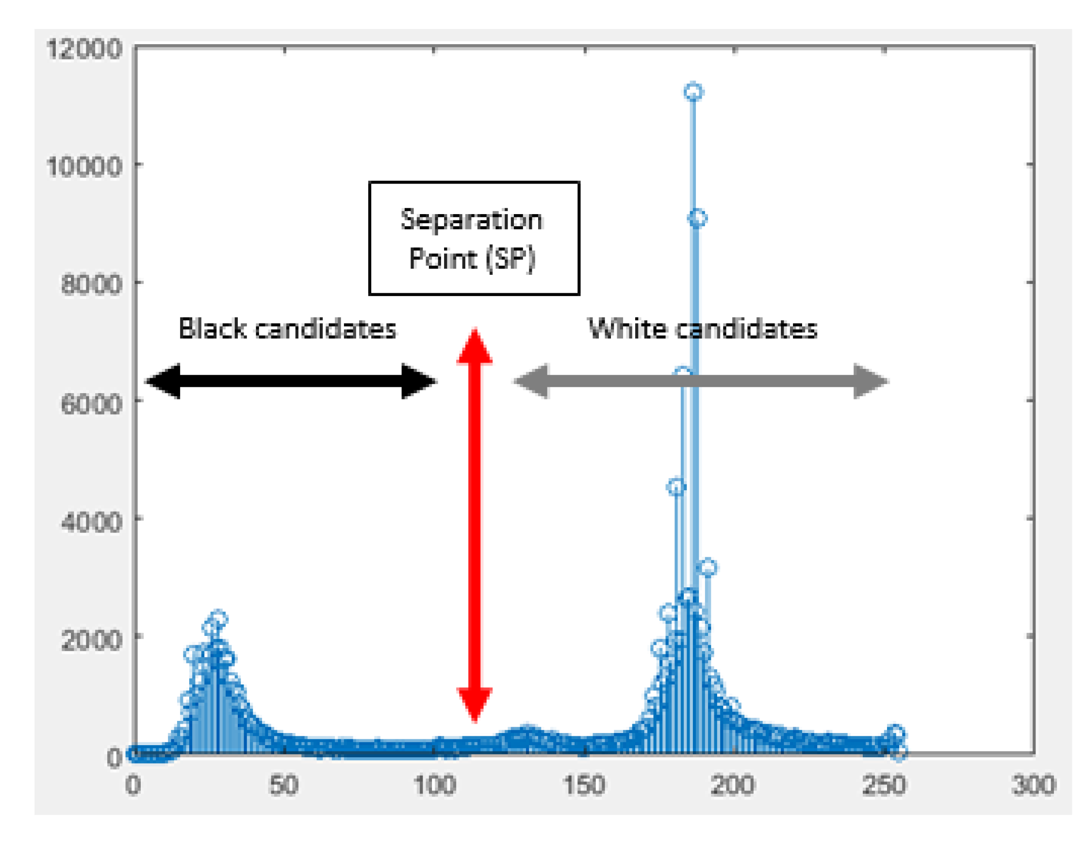
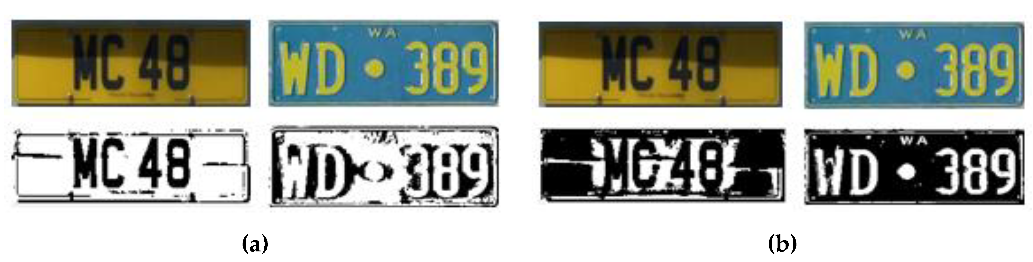
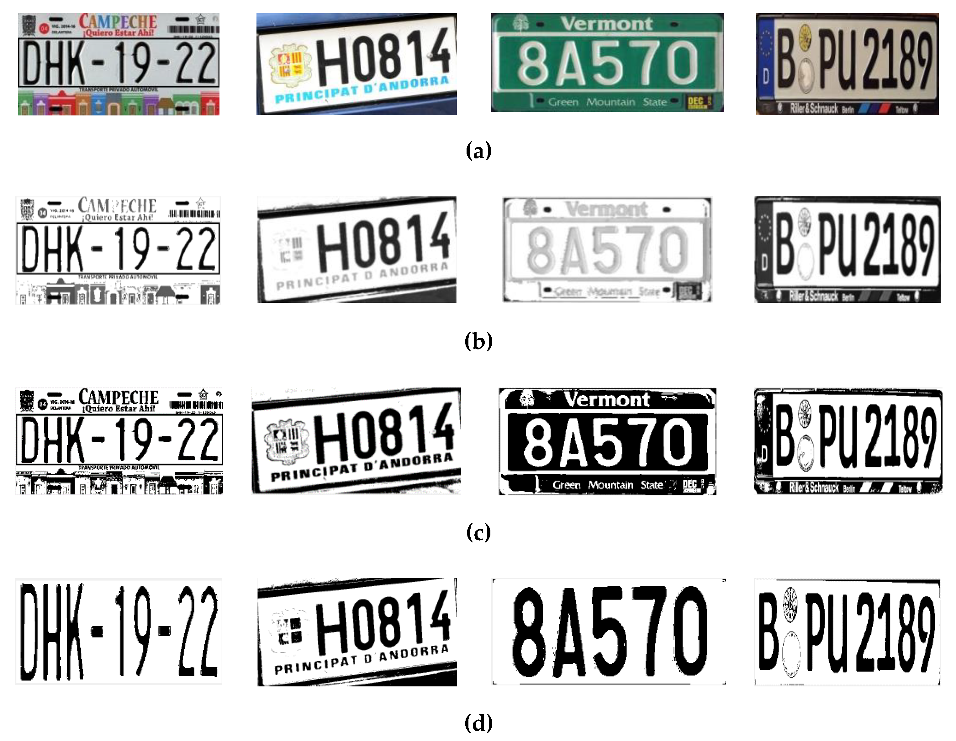
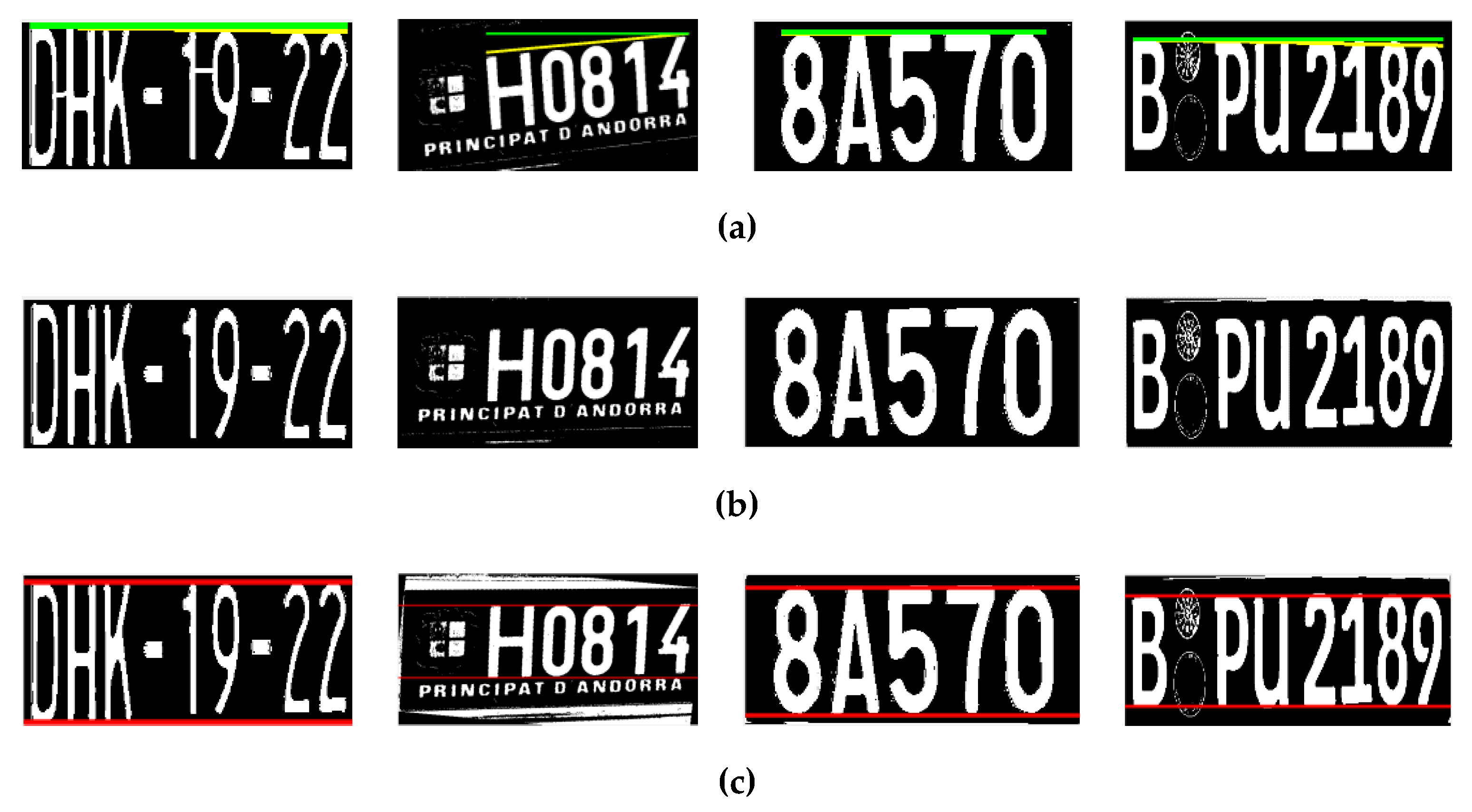
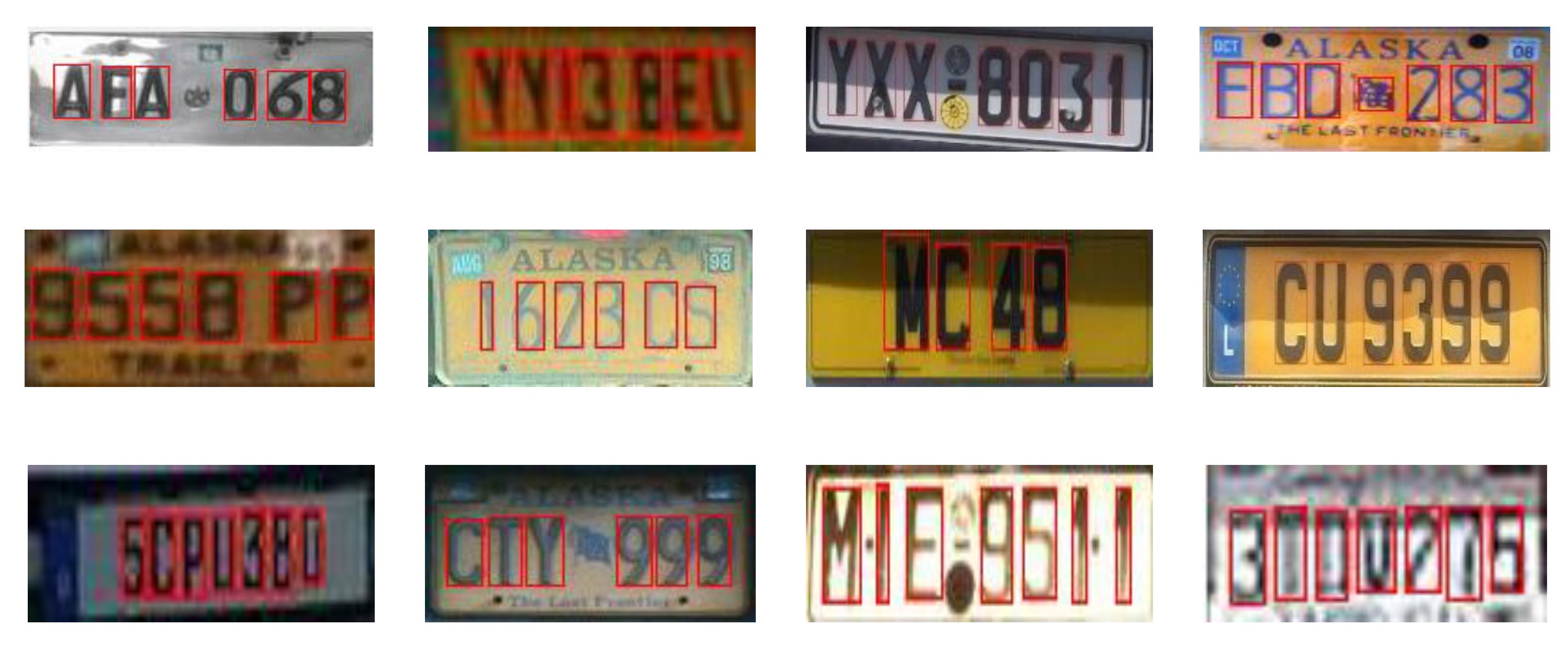
3.1. License Plate Character Segmentation
| Algorithm 1 Foreground polarity detection process |
| Input 1: max1 % max1 represents the color pixel count belongs to LP background |
| Input 2: max2 % max2 represents the color pixel count belongs to LP foreground |
| If (max1 & max2) CG1 |
| If max1 (Ind) > max2 (Ind) |
| FP ← bright |
| Else |
| FP ← dark |
| End |
| Else if (max1 CG1& max2 CG2) || (max1 CG2 & max2 CG1) |
| Output: |
| FP← find {CG2(Ind)} |
| End |
3.2. License Plate Character Recognition
4. Experimental Results and Discussion
4.1. LP Characters Segmentation Results Analysis
4.2. LP Characters Recognition Results Analysis
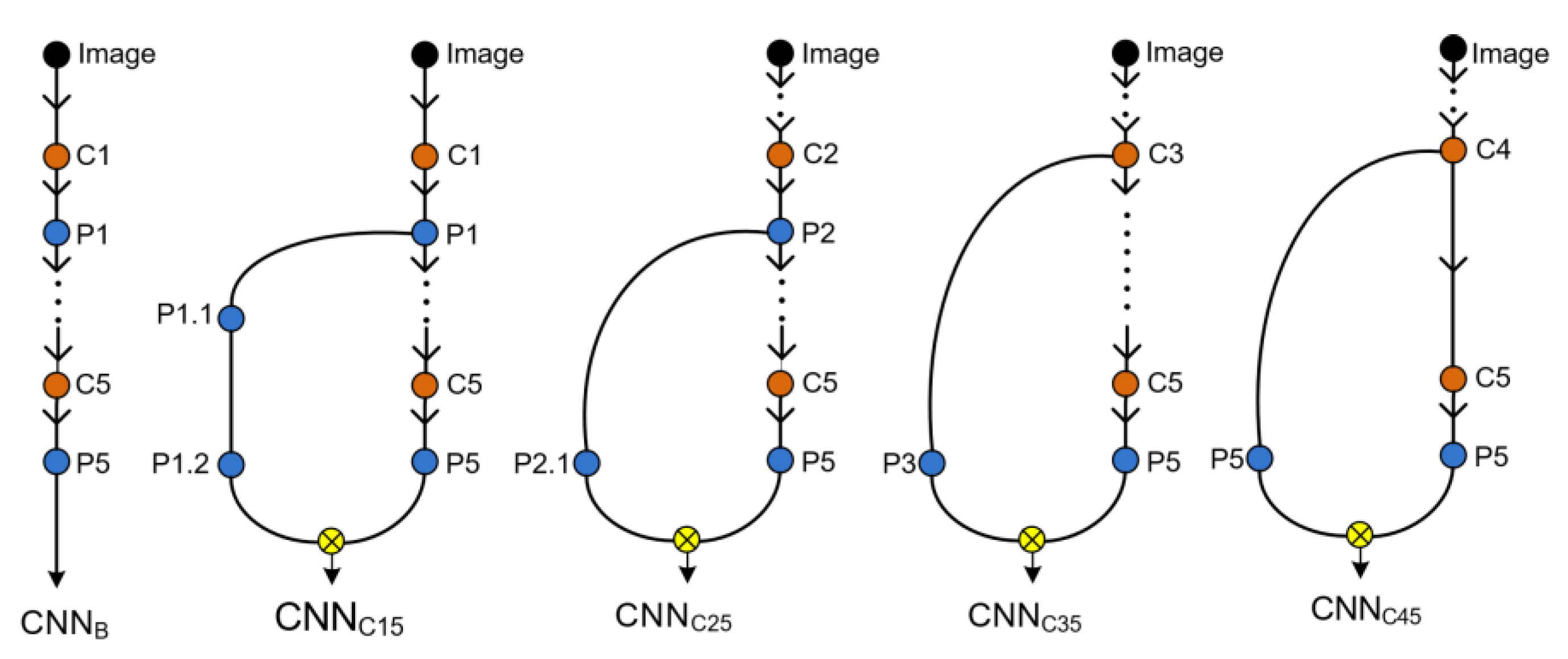
4.2.1. Layers Aggregation Module
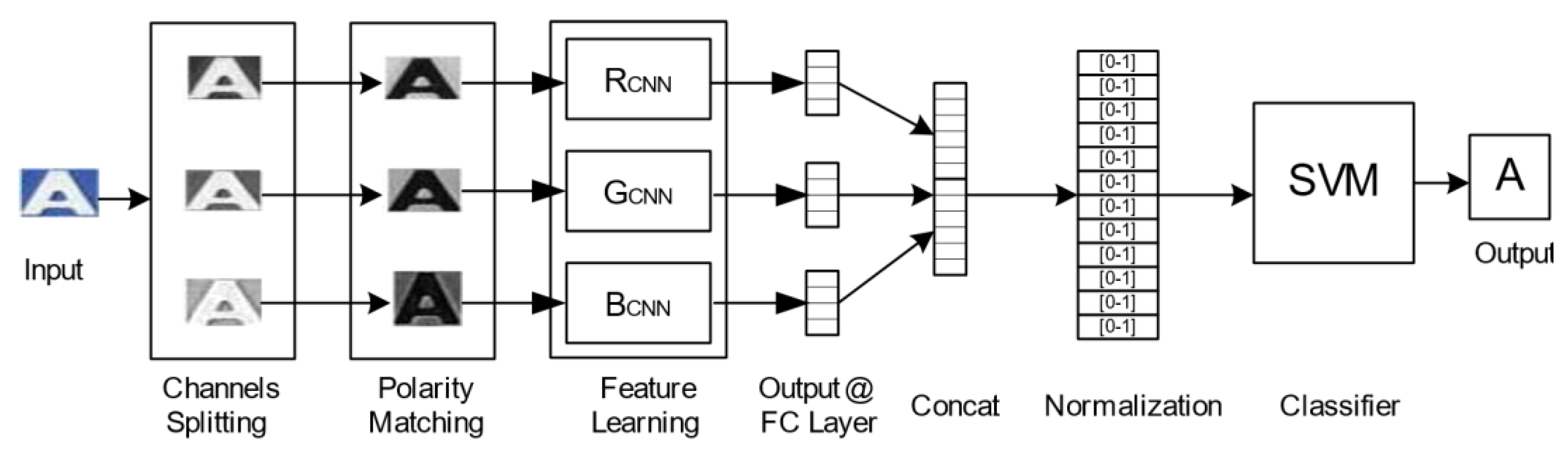
4.2.2. Multi-Channel CNN Architecture Module
4.2.3. Impact of FG-Polarity Matching Module
5. Conclusions
Author Contributions
Funding
Conflicts of Interest
References
- Asif, M.R.; Qi, C.; Wang, T.; Fareed, M.S.; Raza, S.A. License plate detection for multi-national vehicles: An illumination invariant approach in multi-lane environment. Comput. Electr. Eng. 2019, 78, 132–147. [Google Scholar] [CrossRef]
- Asif, M.R.; Chun, Q.; Hussain, S.; Fareed, M.S.; Khan, S. Multinational vehicle license plate detection in complex backgrounds. J. Vis. Commun. Image Represent. 2017, 46, 176–186. [Google Scholar] [CrossRef]
- Asif, M.R.; Qi, C.; Bibi, I.; Sadiq Fareed, M.; Zhang, Z.; Zhang, Z. Performance Evaluation of Local Image Features for Multinational Vehicle License Plate Verification. IEEE Intell. Veh. Symp. Proc. 2018, 2018, 2170–2175. [Google Scholar]
- Saini, M.K.; Saini, S. Multiwavelet transform based license plate detection. J. Vis. Commun. Image Represent. 2017, 44, 128–138. [Google Scholar] [CrossRef]
- Zhang, J.; Li, Y.; Li, T.; Xun, L.; Shan, C. License Plate Localization in Unconstrained Scenes Using a Two-Stage CNN-RNN. IEEE Sens. J. 2019, 19, 5256–5265. [Google Scholar] [CrossRef]
- Shapiro, V.; Gluhchev, G.; Dimov, D. Towards a multinational car license plate recognition system. Mach. Vis. Appl. 2006, 17, 173–183. [Google Scholar] [CrossRef]
- Shapiro, V.; Gluhchev, G. Multinational license plate recognition system: Segmentation and classification. Proc. Int. Conf. Pattern Recognit. 2004, 4, 352–355. [Google Scholar]
- Tian, J.; Wang, R.; Wang, G.; Liu, J.; Xia, Y. A two-stage character segmentation method for Chinese license plate. Comput. Electr. Eng. 2015, 46, 539–553. [Google Scholar] [CrossRef]
- Sasi, A.; Sharma, S.; Cheeran, A.N. Automatic Car Number Plate Recognition. In Proceedings of the 2017 International Conference on Innovations in Information, Embedded and Communication Systems (ICIIECS), Coimbatore, India, 17–18 March 2017; pp. 1–6. [Google Scholar]
- Abedin, M.Z.; Nath, A.C.; Dhar, P.; Deb, K.; Hossain, M.S. License plate recognition system based on contour properties and deep learning model. In Proceedings of the 2017 IEEE Region 10 Humanitarian Technology Conference (R10-HTC), Dhaka, Bangladesh, 21–23 December 2017; pp. 590–593. [Google Scholar]
- Azam, S.; Islam, M.M. Automatic license plate detection in hazardous condition. J. Vis. Commun. Image Represent. 2016, 36, 172–186. [Google Scholar] [CrossRef]
- Barnouti, N.H.; Naser, M.A.S.; Al-Dabbagh, S.S.M. Automatic Iraqi license plate recognition system using back propagation neural network (BPNN). In Proceedings of the 2017 Annual Conference on New Trends in Information & Communications Technology Applications (NTICT), Baghdad, Iraq, 7–9 March 2017; pp. 105–110. [Google Scholar]
- Khan, M.A.; Sharif, M.; Javed, M.Y.; Akram, T.; Yasmin, M.; Saba, T. License number plate recognition system using entropy-based features selection approach with SVM. IET Image Process. 2018, 12, 200–209. [Google Scholar] [CrossRef]
- Pan, M.S.; Yan, J.B.; Xiao, Z.H. Vehicle license plate character segmentation. Int. J. Autom. Comput. 2008, 5, 425–432. [Google Scholar] [CrossRef]
- Ashtari, A.H.; Nordin, M.J.; Fathy, M. An Iranian license plate recognition system based on color features. IEEE Trans. Intell. Transp. Syst. 2014, 15, 1690–1705. [Google Scholar] [CrossRef]
- Hsu, G.S.; Chen, J.C.; Chung, Y.Z. Application-oriented license plate recognition. IEEE Trans. Veh. Technol. 2013, 62, 552–561. [Google Scholar] [CrossRef]
- Gou, C.; Wang, K.; Yao, Y.; Li, Z. Vehicle License Plate Recognition Based on Extremal Regions and Restricted Boltzmann Machines. IEEE Trans. Intell. Transp. Syst. 2016, 17, 1096–1107. [Google Scholar] [CrossRef]
- Bulan, O.; Kozitsky, V.; Ramesh, P.; Shreve, M. Segmentation- and Annotation-Free License Plate Recognition with Deep Localization and Failure Identification. IEEE Trans. Intell. Transp. Syst. 2017, 18, 2351–2363. [Google Scholar] [CrossRef]
- Panahi, R.; Gholampour, I. Accurate Detection and Recognition of Dirty Vehicle Plate Numbers for High-Speed Applications. IEEE Trans. Intell. Transp. Syst. 2017, 18, 767–779. [Google Scholar] [CrossRef]
- Wang, J.; Huang, H.; Qian, X.; Cao, J.; Dai, Y. Sequence recognition of Chinese license plates. Neurocomputing 2018, 317, 149–158. [Google Scholar] [CrossRef]
- Laroca, R.; Severo, E.; Zanlorensi, L.A.; Oliveira, L.S.; Goncalves, G.R.; Schwartz, W.R.; Menotti, D. A Robust Real-Time Automatic License Plate Recognition Based on the YOLO Detector. In Proceedings of the 2018 International Joint Conference on Neural Networks (IJCNN), Rio de Janeiro, Brazil, 8–13 July 2018. [Google Scholar]
- Björklund, T.; Fiandrotti, A.; Annarumma, M.; Francini, G.; Magli, E. Robust license plate recognition using neural networks trained on synthetic images. Pattern Recognit. 2019, 93, 134–146. [Google Scholar] [CrossRef]
- Wang, W.; Yang, J.; Chen, M.; Wang, P. A Light CNN for End-to-End Car License Plates Detection and Recognition. IEEE Access 2019, 7, 173875–173883. [Google Scholar] [CrossRef]
- Comelli, P.; Ferragina, P.; Granieri, M.N.; Stabile, F. Optical Recognition of Motor Vehicle License Plates. IEEE Trans. Veh. Technol. 1995, 44, 790–799. [Google Scholar] [CrossRef]
- Huang, Y.P.; Lai, S.Y.; Chuang, W.P. A template-based model for license plate recognition. In Proceedings of the IEEE International Conference on Networking, Sensing and Control, Taipei, Taiwan, 21–23 March 2004; Volume 2, pp. 737–742. [Google Scholar]
- Jagtap, J.; Holambe, S. Multi-Style License Plate Recognition using Artificial Neural Network for Indian Vehicles. In Proceedings of the 2018 International Conference on Information, Communication, Engineering and Technology (ICICET), Pune, India, 29–31 August 2018; pp. 1–4. [Google Scholar]
- Kocer, H.E.; Cevik, K.K. Artificial neural networks based vehicle license plate recognition. Procedia Comput. Sci. 2011, 3, 1033–1037. [Google Scholar] [CrossRef]
- Huang, Y.P.; Chen, C.H.; Chang, Y.T.; Sandnes, F.E. An intelligent strategy for checking the annual inspection status of motorcycles based on license plate recognition. Expert Syst. Appl. 2009, 36, 9260–9267. [Google Scholar] [CrossRef]
- Wen, Y.; Lu, Y.; Yan, J.; Zhou, Z.; Von Deneen, K.M.; Shi, P. An algorithm for license plate recognition applied to intelligent transportation system. IEEE Trans. Intell. Transp. Syst. 2011, 12, 830–845. [Google Scholar] [CrossRef]
- Raghunandan, K.S.; Shivakumara, P.; Jalab, H.A.; Ibrahim, R.W.; Kumar, G.H.; Pal, U.; Lu, T. Riesz Fractional Based Model for Enhancing License Plate Detection and Recognition. IEEE Trans. Circuits Syst. Video Technol. 2018, 28, 2276–2288. [Google Scholar] [CrossRef]
- Yang, Y.; Li, D.; Duan, Z. Chinese vehicle license plate recognition using kernel-based extreme learning machine with deep convolutional features. IET Intell. Transp. Syst. 2018, 12, 213–219. [Google Scholar] [CrossRef]
- Duan, T.; Du, T. Building an automatic vehicle license plate recognition system. In Proceedings of the International Conference Computer Science, Can Tho, Vietnam, 21–24 February 2005; pp. 59–63. [Google Scholar]
- Lin, C.H.; Lin, Y.S.; Liu, W.C. An efficient license plate recognition system using convolution neural networks. In Proceedings of the 2018 IEEE International Conference on Applied System Invention (ICASI), Chiba, Japan, 13–17 April 2018; pp. 224–227. [Google Scholar]
- Puarungroj, W.; Boonsirisumpun, N. Thai License Plate Recognition Based on Deep Learning. Procedia Comput. Sci. 2018, 135, 214–221. [Google Scholar] [CrossRef]
- Zang, D.; Chai, Z.; Zhang, J.; Zhang, D.; Cheng, J. Vehicle license plate recognition using visual attention model and deep learning. J. Electron. Imaging 2015, 24, 033001. [Google Scholar] [CrossRef]
- RGB Color Space. Available online: https://engineering.purdue.edu/~abe305/HTMLS/rgbspace.htm (accessed on 10 July 2019).
- Krizhevsky, A.; Sutskever, I.; Hinton, G.E. Imagenet classification with deep convolutional neural networks. Adv. Neural Inf. Process. Syst. 2012, 25, 1097–1105. [Google Scholar]
- Simonyan, K.; Zisserman, A. Very Deep Convolutional Networks for Large-Scale Image Recognition. arXiv 2014, arXiv:1409.1556. [Google Scholar]
- Szegedy, C.; Liu, W.; Jia, Y.; Sermanet, P.; Reed, S.; Anguelov, D.; Erhan, D.; Vanhoucke, V.; Rabinovich, A. Going deeper with convolutions. In Proceedings of the IEEE Conference on Computer Vision and Pattern Recognition, Boston, MA, USA, 7–12 June 2015; pp. 1–9. [Google Scholar]
- He, K.; Zhang, X.; Ren, S.; Sun, J. Deep residual learning for image recognition. In Proceedings of the IEEE Conference on Computer Vision and Pattern Recognition (CVPR), Las Vegas, NV, USA, 27–30 June 2016; pp. 770–778. [Google Scholar]
- Szegedy, C.; Vanhoucke, V.; Ioffe, S.; Shlens, J.; Wojna, Z. Rethinking the Inception Architecture for Computer Vision. In Proceedings of the IEEE Conference on Computer Vision and Pattern Recognition (CVPR), Las Vegas, NV, USA, 27–30 June 2016; pp. 2818–2826. [Google Scholar]
- Yu, F.; Wang, D.; Shelhamer, E.; Darrell, T. Deep Layer Aggregation. In Proceedings of the IEEE Conference on Computer Vision and Pattern Recognition (CVPR), Salt Lake City, UT, USA, 18–23 June 2018; pp. 2403–2412. [Google Scholar]
- Sun, Y.; Wang, X.; Tang, X. Deep learning face representation from predicting 10,000 classes. In Proceedings of the IEEE Computer Soc. Conference Computer Vision Pattern Recognition, Columbus, OH, USA, 23–28 June 2014; pp. 1891–1898. [Google Scholar]
- Kong, T.; Yao, A.; Chen, Y.; Sun, F. HyperNet: Towards accurate region proposal generation and joint object detection. In Proceedings of the IEEE Computer Soc. Conference Computer Vision Pattern Recognition, Las Vegas, NV, USA, 27–30 June 2016; pp. 845–853. [Google Scholar]
- Tang, L.; Gao, C.; Chen, X.; Zhao, Y. Pose detection in complex classroom environment based on improved faster R-CNN. IET Image Process. 2019, 13, 451–457. [Google Scholar] [CrossRef]
- Zhang, J.; Shao, K.; Luo, X. Small sample image recognition using improved Convolutional Neural Network. J. Vis. Commun. Image Represent. 2018, 55, 640–647. [Google Scholar] [CrossRef]
- Delforouzi, A.; Pooyan, M. Efficient farsi license plate recognition. In Proceedings of the 2009 7th International Conference on Information, Communications and Signal Processing (ICICS), Macau, China, 8–10 December 2009; pp. 1–5. [Google Scholar]
- Qi, X.; Wang, T.; Liu, J. Comparison of Support Vector Machine and Softmax Classifiers in Computer Vision. In Proceedings of the 2017 Second International Conference on Mechanical, Control and Computer Engineering (ICMCCE), Harbin, China, 8–10 December 2017; pp. 151–155. [Google Scholar]
- He, T.; Li, X. Image Quality Recognition Technology Based on Deep Learning. J. Vis. Commun. Image Represent. 2019. [Google Scholar] [CrossRef]
- Fan, X.; Tjahjadi, T. Fusing dynamic deep learned features and handcrafted features for facial expression recognition. J. Vis. Commun. Image Represent. 2019, 65, 102659. [Google Scholar] [CrossRef]
- TemplateSVM. Available online: https://www.mathworks.com/help/stats/templatesvm.html (accessed on 13 September 2019).
- Medialab LPR Database. Available online: http://www.medialab.ntua.gr/research/LPRdatabase.html (accessed on 25 September 2019).
- Olav’s License Plate Pictures. Available online: http://www.olavsplates.com/ (accessed on 25 September 2019).


| Color Count | Color Group | |
|---|---|---|
| d1 ≥ 0.24 & d3 ≥ 0.24 | B < R > G | |
| d1 < 0.24 & d3 ≥ 0.24 | ||
| d1 ≥ 0.24 & d3 < 0.24 | ||
| d2 ≥ 0.24 & d3 ≥ 0.24 | R < B > G | |
| d3 ≥ 0.24 & d2 < 0.24 | ||
| d1 ≥ 0.24 & d3 < 0.24 | ||
| d1 ≥ 0.24 & d2 ≥ 0.24 | R < G > B | |
| d1 < 0.24 & d2 ≥ 0.24 | ||
| d1 ≥ 0.24 & d2 < 0.24 |
| Layers | Configuration | |||
|---|---|---|---|---|
| Input | FM: 1 | OS: 227 × 227 × 3 | KS: - | S: - |
| Convolution1 | FM: 96 | OS: 55 × 55 × 96 | KS: 11 × 11 | S: 4 |
| Max Pooling1 | FM: 96 | OS: 27 × 27 × 96 | KS: 3 × 3 | S: 2 |
| Convolution2 | FM: 256 | OS: 27 × 27 × 256 | KS: 5 × 5 | S: 1 |
| Max Pooling2 | FM: 256 | OS: 13 × 13 × 256 | KS: 3 × 3 | S: 2 |
| Convolution3 | FM: 384 | OS: 13 × 13 × 384 | KS: 3 × 3 | S: 1 |
| Convolution4 | FM: 384 | OS: 13 × 13 × 384 | KS: 3 × 3 | S: 1 |
| Max Pooling4 | FM: 384 | OS: 6 × 6 × 384 | KS: 3 × 3 | S: 2 |
| Convolution5 | FM: 256 | OS: 13 × 13 × 256 | KS: 3 × 3 | S: 1 |
| Max Pooling4 | FM: 256 | OS: 6 × 6 × 256 | KS: 3 × 3 | S: 2 |
| Concatenation | OS: 6 × 6 × 640 | Layer4 © Layer5 | ||
| FC6 | OS: 1 × 1 × 4096 | |||
| FC7 | OS: 1 × 1 × 4096 | |||
| FC8 | OS: 1 × 1 × 37 | |||
| Country | TLPs | NMCLPs | CSc | FSC | Accuracy, % | Precision, % |
|---|---|---|---|---|---|---|
| Australia | 247 | 242 | 1364 | 18 | 97.98 | 98.70 |
| Canada | 329 | 325 | 1813 | 22 | 98.78 | 98.80 |
| England | 150 | 144 | 856 | 12 | 96.00 | 98.62 |
| Mexico | 106 | 103 | 735 | 07 | 97.17 | 99.06 |
| Pakistan | 397 | 382 | 2387 | 37 | 96.22 | 98.47 |
| Europe | 747 | 732 | 4445 | 75 | 97.99 | 98.34 |
| UAE | 46 | 44 | 237 | 05 | 95.65 | 97.93 |
| USA | 1696 | 1630 | 9880 | 191 | 96.11 | 98.10 |
| Total | 3718 | 3602 | 21717 | 367 | 96.88 | 98.33 |
| Recognition Accuracy, % | |||||
|---|---|---|---|---|---|
| Country | CNNB | CNNC15 | CNNC25 | CNNC35 | CNNC45 |
| Australia | 89.67 | 88.49 | 74.10 | 91.14 | 91.55 |
| Canada | 78.76 | 82.47 | 63.72 | 82.41 | 84.62 |
| England | 85.12 | 84.9 | 72.14 | 84.89 | 88.43 |
| Mexico | 93.47 | 93.47 | 85.71 | 95.78 | 96.19 |
| Pakistan | 83.48 | 84.12 | 67.77 | 85.75 | 90.89 |
| Europe | 90.78 | 91.44 | 85.47 | 91.98 | 93.76 |
| UAE | 88.11 | 88.11 | 87.67 | 89.87 | 91.25 |
| USA | 80.64 | 81.97 | 63.03 | 82.00 | 85.69 |
| Total | 86.25 | 86.87 | 74.95 | 87.98 | 90.30 |
| Recognition Accuracy, % | ||||
|---|---|---|---|---|
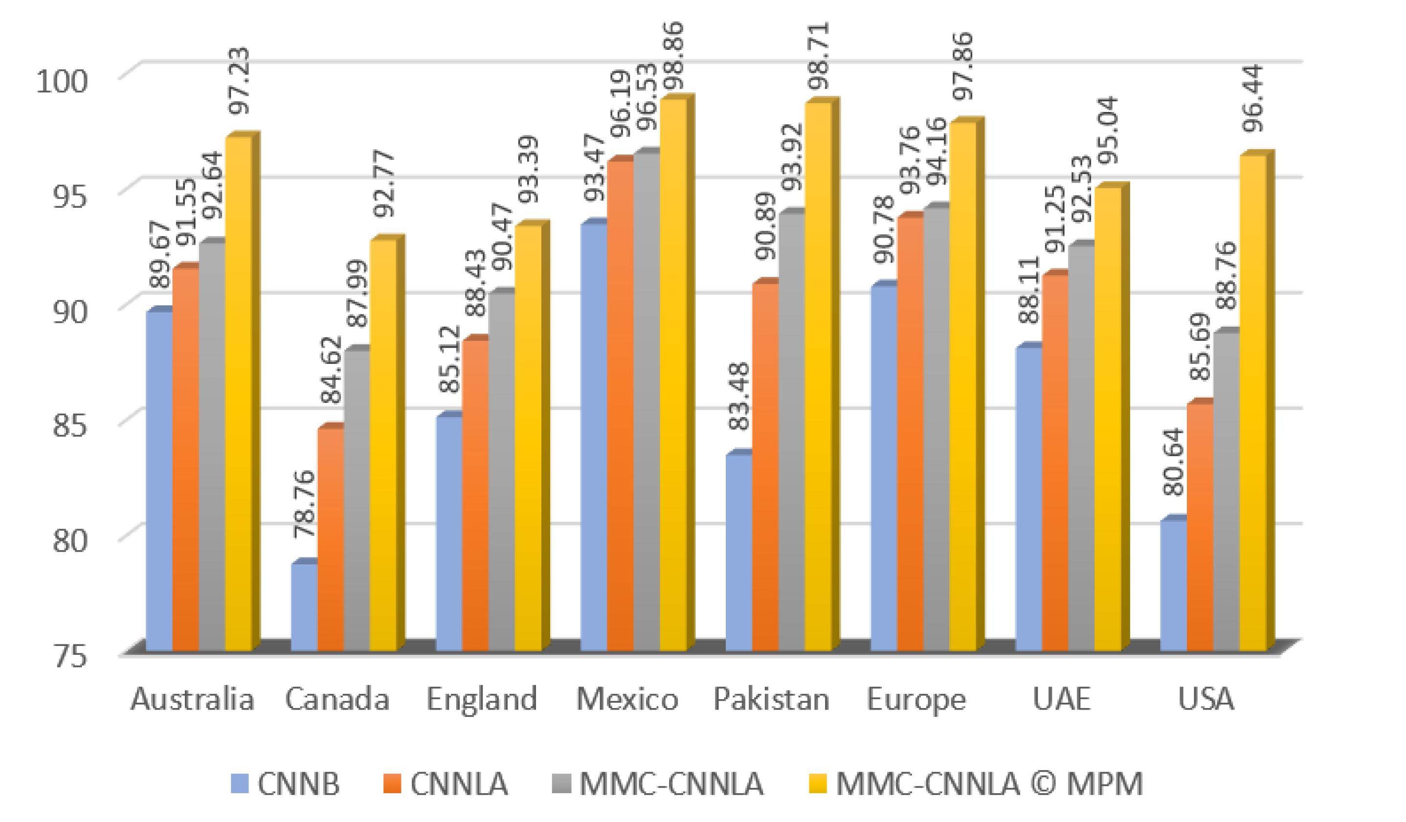
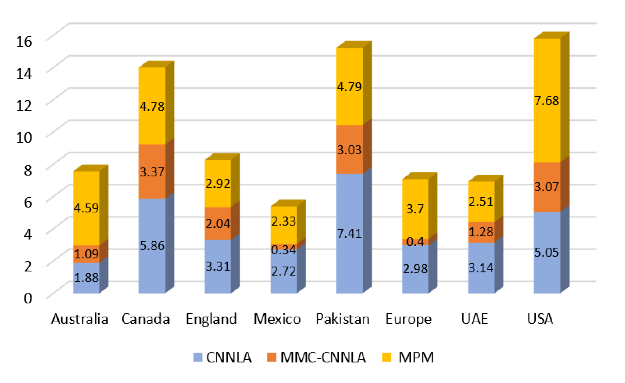
| Country | CNNB | CNN-LA | MMC-CNN-LA | MMC-CNN-LA © MPM |
| Australia | 89.67 | 91.55 | 92.64 | 97.23 |
| Canada | 78.76 | 84.62 | 87.99 | 92.77 |
| England | 85.12 | 88.43 | 90.47 | 93.39 |
| Mexico | 93.47 | 96.19 | 96.53 | 98.86 |
| Pakistan | 83.48 | 90.89 | 93.92 | 98.71 |
| Europe | 90.78 | 93.76 | 94.16 | 97.86 |
| UAE | 88.11 | 91.25 | 92.53 | 93.04 |
| USA | 80.64 | 85.69 | 88.76 | 96.44 |
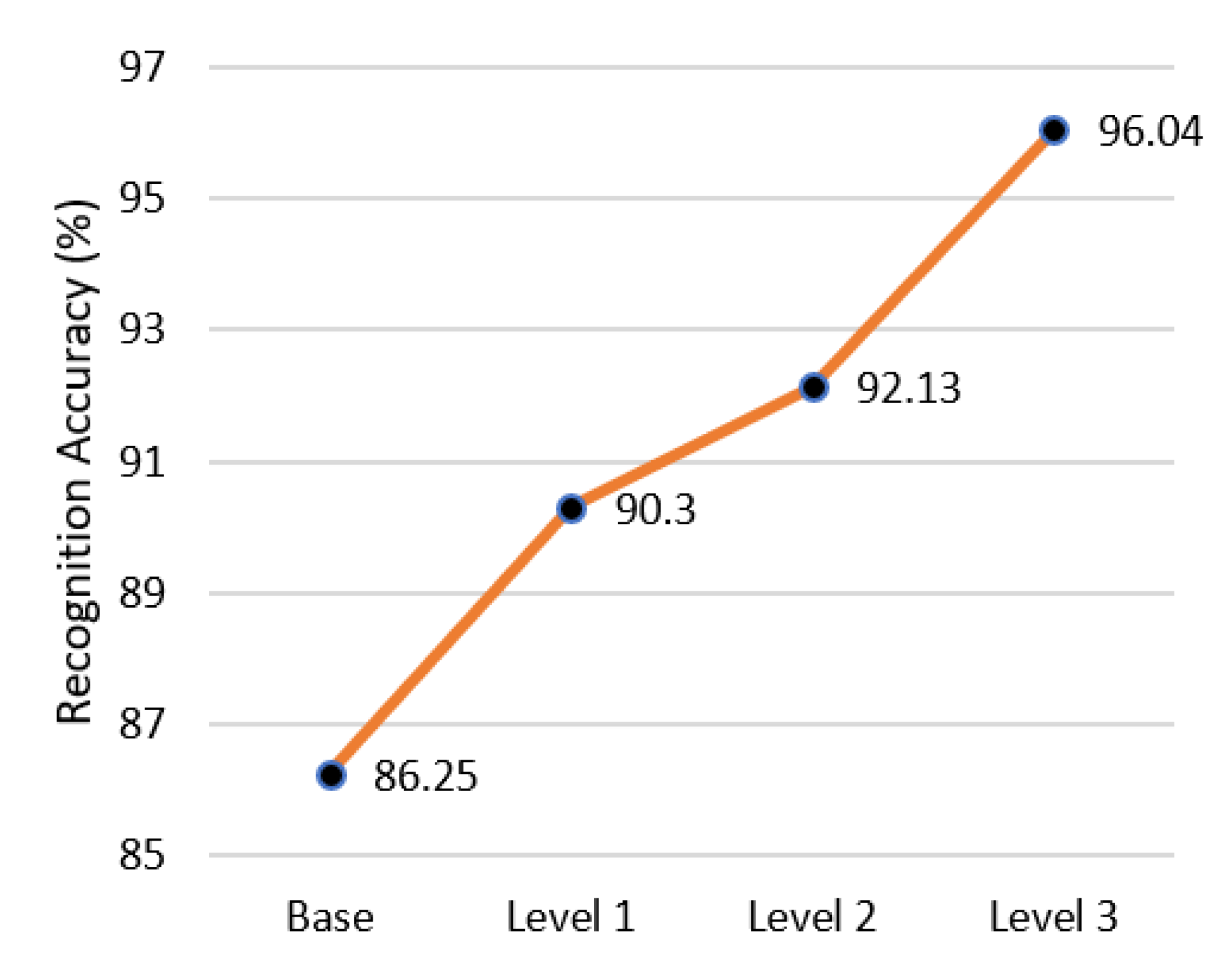
| Total | 86.25 | 90.30 | 92.13 | 96.04 |
© 2020 by the authors. Licensee MDPI, Basel, Switzerland. This article is an open access article distributed under the terms and conditions of the Creative Commons Attribution (CC BY) license (http://creativecommons.org/licenses/by/4.0/).
Share and Cite
Raza, M.A.; Qi, C.; Asif, M.R.; Khan, M.A. An Adaptive Approach for Multi-National Vehicle License Plate Recognition Using Multi-Level Deep Features and Foreground Polarity Detection Model. Appl. Sci. 2020, 10, 2165. https://doi.org/10.3390/app10062165
Raza MA, Qi C, Asif MR, Khan MA. An Adaptive Approach for Multi-National Vehicle License Plate Recognition Using Multi-Level Deep Features and Foreground Polarity Detection Model. Applied Sciences. 2020; 10(6):2165. https://doi.org/10.3390/app10062165
Chicago/Turabian StyleRaza, Muhammad Ali, Chun Qi, Muhammad Rizwan Asif, and Muhammad Armoghan Khan. 2020. "An Adaptive Approach for Multi-National Vehicle License Plate Recognition Using Multi-Level Deep Features and Foreground Polarity Detection Model" Applied Sciences 10, no. 6: 2165. https://doi.org/10.3390/app10062165
APA StyleRaza, M. A., Qi, C., Asif, M. R., & Khan, M. A. (2020). An Adaptive Approach for Multi-National Vehicle License Plate Recognition Using Multi-Level Deep Features and Foreground Polarity Detection Model. Applied Sciences, 10(6), 2165. https://doi.org/10.3390/app10062165