A Comprehensive Report on Ultrasonic Attenuation of Engineering Materials, Including Metals, Ceramics, Polymers, Fiber-Reinforced Composites, Wood, and Rocks

Abstract

In this paper, ultrasonic attenuation of engineering materials is evaluated comprehensively, covering metals, ceramics, polymers, fiber-reinforced composites, wood, and rocks. After verifying two reliable experimental methods, 336 measurements are conducted and their results are tabulated. Attenuation behavior is determined over broadband spectra, extending up to 15 MHz in low attenuating materials. The attenuation spectra are characterized in combination with four power law terms, with many showing linear frequency dependence, with or without Rayleigh scattering. Dislocation damping effects are re-evaluated and a new mechanism is proposed to explain some of the linear frequency dependencies. Additionally, quadratic and cubic dependencies due to Datta–Kinra scattering and Biwa scattering, respectively, are used for some materials to construct model relations. From many test results, some previously hidden behaviors emerged upon data evaluation. Effects of cold working, tempering, and annealing are complex and sometimes contradictory. Comparison to available literature was attempted for some, but most often prior data were unavailable. This collection of new attenuation data will be of value in materials selection and in designing structural health monitoring and non-destructive inspection protocols.

1. Introduction

Non-destructive evaluation (NDE) methods based on stress wave propagation have contributed to quality assurance and failure prevention in many industries [1,2,3]. The methods include ultrasonic testing (UT), which uses active interrogation of target components, and acoustic emission (AE) testing, which relies primarily on “acoustic” signals emitted from the target. In recent years, their roles have expanded into continual monitoring and preventive maintenance of wide-ranging products and infrastructures, offering useful tools for structural health monitoring [4,5,6,7]. As the size of structures being inspected increases, the attenuation of stress waves becomes a concern, especially for components of modern fiber-reinforced composites and other high damping materials. In a preceding report [7], a section was devoted to collecting available data on structural alloys, polymers, and fiber-reinforced composites. Despite long-standing scientific and engineering interests in this subject going back to the work of Mason and McSkimin in the 1940s [8], available ultrasonic attenuation data were found to be limited. Most of the attenuation values collected in [7] were for longitudinal waves, while the data for transverse waves were even more sparse, lacking an adequate theoretical foundation, as appropriate diffraction correction has been unavailable. As data from some reports were given as ranges in [7], the total tabulated data count exceeded 80, but this number was still less than 200 for only about 40 different types of materials. Most polymer data, with about 50 being available in [9,10,11], were not included, in part because the test frequency was in the low kHz region or below and was often unidentified. Technical standards for their measurements and validation were also inadequate [12,13]. In order to fill the gap in the presently inadequate database, a study was initiated examining experimental techniques and which culminated with a comprehensive report.

Papadakis [14,15] provided a thorough review of this subject and application examples of a buffer rod method, which he and his colleagues had developed earlier [16]. Their method and its variations have been used by many works cited in [7], including ASTM Standard C1332 [12], as well as in [17,18,19,20,21,22,23,24,25,26]. Margetan et al. [27] published a tutorial for another approach for attenuation measurement, namely the immersion methods. While these methods require advanced ultrasonic instrumentation capable of precise sensor–sample alignment, water coupling allows the inspection of curved surfaces of engineering components. Margetan and his coworkers [28,29,30,31] applied the methods to detect the hard inclusions in aerospace Ti alloys and to evaluate the cleanliness of steel samples.

Here, it is necessary to define terms that will be used, as wave attenuation is characterized using several different parameters. Attenuation coefficient α is often used in UT and AE to represent an exponential decay. Taking the initial and attenuated wave amplitude in the displacement, A_o and A, and the propagation distance, x, we have

A = A_o exp (−α x).

(1)

The commonly used unit for α is dB/m. However, it is sometimes convenient to use Np/m, whereby 8.686 dB = 1 Np. Np stands for Neper, a non-dimensional unit that is useful in numerical computation. In this work, only longitudinal waves are considered and no subscript is used for wave types. Previously in [7], α was denoted by α_p. This α is related to the damping (or loss) factor η by η = αλ/π, where λ is the wave length and α is given in the unit of Np/m. Here, 2πη is the ratio of energy dissipated per cycle to maximum energy stored per cycle; η is often denoted as Q⁻¹ in seismology [32] and in electrical engineering, and η is also equal to the loss tangent, tan δ. This tan δ is defined as the ratio of the imaginary part (E”) to the real part (E’) of a complex elastic modulus, E* = E’ − iE”, with i2 = −1.

The damping factor (or loss tangent) is often used in dealing with vibration damping at lower frequencies, especially in polymers, where attenuation arises from viscous damping or hysteretic behavior. When η is independent of frequency, the attenuation coefficient due to viscous damping, α_d, is given by

α_d = C_d f = π η/λ = π η f/v_L,

(2)

where f is the frequency and v_L is the longitudinal wave velocity; that is, attenuation coefficient α_d increases linearly with frequency, with C_d as a constant for attenuation due to damping of longitudinal waves. This α_d, which is proportional to frequency, was initially attributed to elastic hysteresis [8], and early works on damping factors (η = Q⁻¹) of metals were tabulated in [32]. The damping phenomena were also called internal friction, for which log decrement ∆ = ln (A_o/A) was commonly used and ∆ = π η.

The origin of α_d was correlated to dislocation damping in metals [33,34], known as the Koehler–Granato–Lücke (KGL) theory. Dislocation damping is attributed to phonon and electron drags in dislocation oscillations, thermoelastic damping, and mode conversion losses. This and related topics were thoroughly reviewed in [35,36,37], and most available experimental data were compiled in a handbook by Blanter et al. [37]. Additional works on ultrasonic absorption not cited in [37] also demonstrated that (i) magnetic damping effects constitute the bulk of α_d in a steel [38], (ii) dislocation damping increased with plastic strain in Al single crystals [39], and (iii) α_d in pure Fe diminished with annealing [40]. Material damping at lower frequencies is an important issue in structural design. Sugimoto provided a review with a compilation of the Q⁻¹ values vs. tensile strength for 25 alloys [41]. More recently, Blanter and Golovin [42] gave an updated review of this topic and covered high damping metals in depth. In a book on high intensity ultrasound technology, Abramov [43] provided damping data and showed that the damping factors of common metals, such as Al, Cu, Ni, Fe, and Zn, exceed 0.01 at high strain amplitudes in excess of 10⁻⁴; that is, these metals under high intensity ultrasound (below ~100 kHz) have damping factors higher than that of polymethyl methacrylate (PMMA) under normal ultrasonic test conditions (i.e., strain amplitude of ~10⁻⁷). Methods for testing high damping materials were reviewed in [44]. These works demonstrated that materials with low ultrasonic attenuation, such as Al, Mg, and Fe-Cr alloys, can double as high damping materials at low frequencies and at high strain amplitude [41,42,43,44].

For polymers, this hysteresis effect comes from molecular rearrangements [9,10]. An example of the frequency dependence of this hysteretic damping is shown in Figure 1 for PMMA. In this plot, data points from multiple sources are combined, including Kline [19], Pouet and Rasolofosaon [24], Carlson et al. [25], and Treiber et al. [26], resulting in a linear regression fit with C_d = 85.9 dB/m/MHz (shown by the blue dotted line). The data points formed two groups, with a smaller slope for Kline’s older collected data from six studies and a larger slope for another group that was more recent [24,25,26]. Data from both groups exhibited linear frequency dependence in the MHz range. However, the damping factor started to increase below 1 MHz by a factor of 3 to 5, showing a maximum at 50 Hz (3 Hz for torsional vibration) [7]. For rocks, attenuation studies covered similarly wide frequency ranges, and α_d was found to show linear frequency dependence from 1 kHz to 1 MHz; that is, Q values were constant [45].

Scattering is another cause of wave attenuation. Rayleigh scattering that depends on the fourth power of frequency, f⁴, arises from random scattering centers, such as grain boundaries and distributed second phase particles [8]. This occurs when the distance between scattering centers, d, is much less than λ, or λ >> d. For single phase alloys, polycrystalline grain size is used as d, which is of the order of 10 to 100 µm for most structural metallic alloys. Thus, this Rayleigh scattering effect, denoted by the attenuation coefficient due to scattering, α_s, becomes significant above 5 to 10 MHz. Because of the 4th power frequency dependence, this attenuation effect shows a steep decrease with decreasing frequency, often becoming negligible in the low MHz region. This behavior was reported by [8,18,20,46]. Using a constant C_R for Rayleigh scattering, we have

α_s = C_R f⁴.

(3)

Mason and McSkimin [8] used the sum of α_d and α_s to represent their attenuation data for large-grained Al. This is given as

α = α_d + α_s = C_d f + C_R f⁴,

(4)

and will be referred to as the Mason–McSkimin relation.

Stanke and Kino [47] formulated a unified theory, which provides a smooth transition between three types of scattering in Rayleigh, stochastic, and geometric regions. Stochastic scattering gives f²-dependence, and is applicable when the wave length λ is of the order of the mean spacing of scattering centers, such as grain boundaries and second-phase particles; this is above 20 MHz for typical metals. The geometric scattering types appear to be insignificant in usual NDE applications below 20 MHz and are not considered in this work. Other power law attenuation effects may exist and can be described as α_n = C_n fⁿ. This has been used when it is needed to fit experimental observation. It is known that water attenuation follows the quadratic form, while other liquids exhibit slightly lower n values [1,48,49]. For the case of n = 2, attenuation can also arise from dislocation damping in crystalline solids [20,33,34,35,36], with α written as

α = C₂ f².

(5)

That is, the KGL theory predicts quadratic frequency dependence, and it is necessary to investigate the mechanisms of dislocation damping, which predict the linear frequency dependence, as in the case of polymer damping. This will be discussed in the next section.

Another quadratic frequency dependence of attenuation was observed in particulate–epoxy composites. Kinra et al. [50] observed a sharp rise in attenuation with frequency using 0.3-mm diameter glass spheres finely distributed in epoxy matrix. The α data for the case of 0.451 volume fraction is plotted in Figure 2a after converting the unit for α into dB/m. A second-order polynomial curve fits the data well, with R² = 0.987. This is a combination of Equations (2) and (5), or

α = C_d f + C₂ f²,

(6)

with C_d = 36.3 dB/m/MHz and C₂ = 545 dB/MHz². This will be referred to as the Datta–Kinra relation (with or without C_d term), as it is based on theoretical works by Datta [51,52]. These types of spectra were seen for gray cast iron data, in addition to 26 other cases.

For unidirectional fiber-reinforced composites, Biwa and coworkers [53,54] modeled longitudinal wave attenuation in the normal fiber direction and provided graphical data of a scattering cross-section vs. frequency (both in normalized values). Reading selective data points from [53] and converting the frequency for the case they analyzed, Figure 2b shows the results. Biwa data can be fitted well (R² = 0.998) to a cubic frequency dependence, or

α = C₃ f³,

(7)

with C₃ = 550 dB/m/MHz³. Again, the damping term is usually non-zero, giving the Biwa relation given by

α = C_d f + C₃ f³.

(8)

In the present study, this Biwa relation fitted to eight out of 13 observed composite attenuation datasets in the surface normal direction. In one of them (Kevlar composite), the cubic spectrum (Equation (7)) best described the attenuation.

In early attenuation studies of metals, viscous damping effects were shown to be low by Mason and McSkimin [8] and others (see [7,14] for earlier works). Krautkramer’s book [1] listed α values as less than 10 dB/m at 2 MHz for most structural alloys (except for copper-based alloys) in the first edition in 1969. In subsequent years, research activity on this topic, especially below 5 MHz, has been sparse. In addition to absorption studies noted above [37,38,39], Smith et al. [18] separated α_d terms of steels of various carbon (C) contents. The levels of attenuation were low, with C_d values of 0.7 to 3.5 dB/m/MHz. In most other attenuation studies, only the scattering terms have been examined. However, some works reported results showing that it is unwise to ignore the damping term. Figure 3 gives some examples. Observed attenuation coefficients are plotted as circles (in blue or red) for a low-C steel (Figure 3a, with data from [55]) and for pure niobium (Figure 3b, with data from [56]). For steel, Ahn and Lee [55] normalized 0.2% C steel samples at 900 and 1100 °C, and obtained α values for 5 to 9 MHz, fitting them using a power law, with n measuring approximately 1.5. However, such power law fits have no rational basis from existing theories. These data sets can be modeled using the Mason–McSkimin relation (Equation (4)), assuming that the low-frequency region possesses linear frequency dependence from damping, while the Rayleigh scattering law is obeyed at higher frequencies. The fitted data points are shown by blue or red + symbols, while blue or red dots represent the extension of the linear fit at low frequencies. In the niobium (Nb) case, the data from Zeng et al. [56] is plotted in Figure 3b, indicating α values for two grain sizes (blue for 32 µm and red for 60 µm). Here, available Nb data jumps from 9 to 20 MHz, giving two frequency bands. Zeng et al. [56] compared their data sets with the Stanke–Kino theory [47], but no match was achieved. Using the Mason–McSkimin relation, it is possible to combine damping and scattering components, as shown by blue or red + symbols in Figure 3b. The match was poorer than for steel, however, as the frequency range extends to 27 MHz in this Nb study. While the combined damping–scattering attenuation apparently rationalizes the observed behavior, no theoretical basis is currently available to explain the level of damping, including the KGL theory noted above [33,34,35,36,37].

Since the damping term was not often utilized after 1960 outside the composite field, one of the objectives of the present study is to examine how broadly the Mason–McSkimin relation exists in various materials. It is anticipated that more detailed studies on dislocation effects, including atomistic or molecular dynamic simulations, will be required to establish improved quantitative mechanisms for damping. The extent of applicability of Datta–Kinra and Biwa relations is also of interest as these have not been tested with real attenuation data. These three relations (Mason–McSkimin, Datta–Kinra, and Biwa) are named in this report. Other aims of this work are to experimentally obtain the attenuation coefficients (α) of a wide range of materials in the low MHz range (below 15 MHz), so as to present them in tabular form, to give information that is useful in material selection, and to provide rational interpretation of attenuation behavior. This information will also aid in improving model calculations for distance–amplitude curves for UT and predicting the detectability of AE signals on large structures. Over 300 samples were used, mainly based on the availability in the author’s laboratory, as well as some new acquisitions. Experimental procedures describe transmission difference methods used for attenuation measurements without requiring the reflectivity of interfaces. The Results and Discussion section provides separate tables for different types of materials, metals (steels, non-ferrous alloys, and cast iron), polymers and wood, fiber-reinforced composites, and ceramics and rocks. This part covers general observations and includes comments on peculiar material behavior observed for some groups, such as cold-worked metals and cast iron. Also noteworthy is a transition discovered in mortar spectral results, which changed from the Mason–McSkimin to Datta–Kinra spectrum when void content exceeded 20%. This represented a change from independent to multiple scattering.

2. Dislocation damping

Dislocation damping has been analyzed based on the Koehler vibrating string model [33]. Koehler–Granato–Lücke (KGL) formulation showed a linear frequency dependence of damping factor η below the resonance frequency of around 20 MHz [34,35,36]. In terms of attenuation coefficient α, this becomes quadratic frequency dependence through Equation (1). Heiple and Birnbaum [57] derived an explicit equation for this linear part between logarithmic decrement (∆ = π η) and angular frequency. The logarithmic decrement for Cu was measured in multiple studies at kHz frequencies. At 20 to 25 kHz, ∆ was found to vary on the low side, ranging from 0.001 [58] to 0.0037 [57] and as high as 0.08 [59], with a median value of 0.007. This ∆ range agreed with the prediction of the KGL model using the dislocation drag factor obtained from theory, experiments and atomistic simulations [60,61,62]. Low-frequency internal friction studies used a strain amplitude range of 10⁻⁷ to 10⁻⁵ [58,59,60], but one study used an amplitude of up to 3 × 10⁻⁴ [58]. In ultrasonic attenuation studies, the strain amplitude is slightly lower at 10⁻⁶ to 10⁻⁷, since most transducers can only generate 1 to 10 nm peak output [63] and samples are over 10 mm. The two approaches cover comparable strain amplitude ranges. These kHz data were extrapolated to 1 MHz and converted to α values to compare them with ultrasonic attenuation. The α values from internal friction studies were 0.22 to 8.65 dB/m and the median α was 1.5 dB/m at 1 MHz. In contrast, ultrasonically obtained α values for Cu were 3–100 times higher and typically exhibited the linear frequency dependence (except in two cases in a slightly cold-worked plate). The linear frequency dependence of α was the dominant feature of the present study for various solids. Thus, it is necessary to explore another source of dislocation damping that depends linearly on frequency.

When pinned dislocation segments are cyclically stressed, they oscillate, as shown in Figure 4a. It is assumed that they have a constant segment length, L, and are distributed uniformly in space. Low lattice resistance for dislocation motion in solids with non-local bonding is also assumed, as shown by Gilman [64]. Starting from a straight line at stress position 0 and at time 0, each segment bows out to the left in the first quarter-cycle under applied stress (Figure 4b) and becomes a series of circle segments at position 1 and time 1. Between 0 and 1, stress increases to the positive peak and work is added by moving the dislocation segments while lengthening the segments, which increases the elastic energy stored in the solid medium. The added work, shown in Figure 4c, is lost as heat. Between times 1 and 2, the dislocation returns to the straight line (position 2). This is driven by the shrinkage of the lengthened dislocation as the dislocation segments are moving against positive stress. This is repeated from positions 2 to 4 in reverse manner, again generating energy loss in the form of work done by the moving dislocation segments, pushed by negative applied stress. As will be shown below, dislocation motion is quasi-static, but the dislocation drag term still acts against the motion. For each cycle, energy loss occurs twice during the positive and negative half-cycles, contributing to damping, which is proportional to frequency. This linear behavior originates from the work caused by dislocation motion during each half-cycle. The amount of work caused by the bow-out process can be calculated from the basic dislocation theory [65]. A bowed-out segment with Burgers vector magnitude, b, is shown in Figure 5 under shear stress τ acting on the slip plane. The distance of the bow-out is equal to length from A to B, defined as [AB]. Here, square brackets indicate length. L is equal to [CD], and the radius of the curvature of the bowed-out segment (arc CBD) is denoted as R = [OB] = [OC] = [OD]. The angle 2θ is defined by lines OC and OD. For this geometry, R is given by

R = (L/2)/sin θ.

(9)

The force on the bowed-out segment (arc CBD) is equal to τ bL, and this is balanced by the opposing components of the line tension (= 2a_T Gb² sin θ), where a_T is a line-tension constant of 0.5 and G the shear modulus. Expressing stress using a strain a_S with the shear modulus G, or τ = a_S G, and using Equation (9), we have [65]

τbL = a_S GbL = 2a_T Gb² sin θ = 2a_T Gb²L/2R,

(10)

which reduces to

a_S R = a_T b,

(11)

which relates the strain amplitude a_S to R; that is, given a_S and pinned segment length L, the values of θ and R can be determined, allowing one to calculate the area of the bow-out A_B (bounded by ACBD), as below.

A_B = R²(2θ − sin 2θ)/2

(12)

This leads to the work done by each bow-out by multiplying τ b/2 = a_S Gb/2. Here, a factor of half is needed because applied stress is cyclic, and another factor of half is also needed since the second quarter-cycle contributed no work. It should also be noted that A_B/L corresponds to the average distance of dislocation motion. When the work done per half-cycle, a_S Gb A_B/4, for each elemental volume of L³ is doubled (for positive and negative motion) and divided by L³, the unit volume value of work done per cycle is obtained. The applied strain energy per unit volume per cycle is G a_S²/2. The ratio of work done to the applied strain energy gives the damping factor η at the strain amplitude a_S by adding 2π in the denominator, since η = (energy loss)/2π (stored energy). Then, one gets

η = (a_S Gb A_B/2)/(2π Ga_S²L³/2) = b A_B/2π a_S L³.

(13)

For a_T = 0.5, G = 26 GPa, b = 0.3 nm, and L = 10 µm, the work done, applied strain energy, and damping factor were calculated for a_S of 2 × 10⁻⁸ to 10⁻⁵ and plotted in Figure 6.

For the strain amplitude range of 2 × 10⁻⁸ to 10⁻⁵, η values remain almost unchanged at 0.027. This is a very high value for metals and is high even for polymers. When the wave length of Al is used at 1 MHz, the η value corresponds to α = 117 dB/m. The range of a_S is wide and the maximum a_S corresponds to stress, which is one-third of the Orowan stress of unstable bow-out (or break-away stress). Here, the maximum bow-out distance was 0.86 µm under 260 kPa, indicating the maximum dislocation velocity was 3.4 m/s at 1 MHz excitation. This is about 1000 times slower than the shear wave velocity of Al (3.1 km/s) and the dislocation motion can be regarded as quasi-static. On the other end of low a_S, the maximum bow-out under 0.52 kPa was 2.1 nm, with a dislocation velocity of 8.4 mm/s. Still, the same level of damping is predicted. Such dislocation velocities were well below the velocities limited by the dislocation damping coefficient, B. Hikata et al. [60] experimentally obtained B = 5.0 × 10⁻⁶ Pa·s at 300 K, while Olmsted et al. [61] found B = 1.4 × 10⁻⁵ Pa·s at 342 K via a molecular dynamics (MD) approach. Another MD result [62] gives B = 2.8 × 10⁻⁵ Pa·s at 100 K (averaging screw and edge values). At 260 kPa, these B values predict dislocation velocities of 5.5 to 156 m/s, all exceeding the maximum dislocation velocities needed in the proposed bow-out mechanism of dislocation damping; that is, the bow-out damping mechanism operates in the quasi-static regime.

When L is reduced to 1 µm, η values are almost unchanged at 0.027. Each elemental volume contributes less, but their number increase by 1000-fold. When a_T is reduced, dislocation becomes flexible and damping increases substantially. Lower values of a_T (of 0.1 to 0.5) are sometimes used in atomistic calculations [66]. At a_T = 0.1, the work done is 90% of the applied elastic energy, increasing η by five-fold; that is, η varies in proportion to a_T. It appears that low line tension of a_T below 0.1 is unrealistic. Thus, as long as dislocations are mobile with low stress, oscillating dislocations provide the basis for rationalizing the linear frequency-dependent damping behavior. However, the lack of effect of pinning length reduction on η values is surprising, as this was initially thought to offer a clue in understanding cold working effects. The explanation of two contradictory cold working effects will have to be sought elsewhere [67].

The dislocation bow-out mechanism proposed above is based on shear deformation, so the attenuation is for the shear wave propagation. However, the attenuation also applies to the longitudinal wave mode, as the normal and shear stresses (or strains) are related via the Taylor factor, M (or 1/M) [68]. Consequently, the strain energy and external work terms are unaffected by the coordinate transformation involved; that is, the attenuation coefficients from dislocation damping are identical in the longitudinal and shear modes of wave propagation. Mason and McSkimin [8] and Papadakis [41] made the only known direct comparison of attenuation coefficients between the longitudinal and shear modes, reporting 2.5- to 8-fold increase for the shear attenuation for five metallic materials. However, most of these were taken at 10–15 MHz, where the Rayleigh scattering caused the attenuation. Further study is needed to find if similar differences persist at lower frequencies, as was the case of 2017 Al alloy [8]. If so, the above prediction of the bow-out mechanism will have to be reconsidered.

Many mechanisms can lower attenuation to the ranges of observed α values, including higher lattice resistance to dislocation, dislocation–dislocation interactions, solute atmospheres, and distribution of the second phase. However, the dislocation bow-out mechanism introduced here does provide a new approach to account for the linear frequency dependence of the attenuation coefficient in non-viscoelastic solids. The main limitation of this mechanism is its inability to explain the attenuation of hard solids. These have low dislocation mobility due to their intrinsic strength and their linear attenuation behavior remains unresolved.

3. Materials and Experimental Procedures

Attenuation measurements were conducted on solid samples with two parallel surfaces. Over 300 tests were completed and their results will be reported in the following sections. Most materials tested were on hand from previous research or instructional work, with detailed characteristics for some, but without for most. About a dozen samples were newly acquired for testing, mainly of rocks and wood materials to supplement existing stock. While some had known sources, chemical compositions, and heat treatment history, most were only identifiable by material types. In order to provide indications of material conditions, hardness tests (Vickers and Rockwell) were conducted for metal samples. For others, density was measured. The longitudinal wave velocity was determined for all, giving additional clues to material conditions. In limiting cases when multiple samples are available, heat treatment was applied to find the effects of microstructural changes on attenuation. However, metallography was not used, as suitable sample preparation facilities were unavailable.

Attenuation measurements were utilized through transmission setups. This method uses damped, wideband transducers, as in the buffer rod methods of Papadakis et al. [16], and relies on two transducer setups, as in [26]. However, the present method avoids using the reflectivity parameter in the attenuation calculation [16,26]. The present approach uses setups shown schematically in Figure 7a. Also included is a photograph of one of the jigs used to hold samples (with an Al rod shown) and transducers (Figure 7b). Setup 1 is used for direct contact of the transmitter and receiver, giving the voltage output V₁ from the receiver as a result of transmitter excitation by a pulser. This is often called face-to-face testing. Setup 2 contains sample 1 between the transmitter and receiver, while Setup 3 contains sample 2 between the transmitter and receiver. These yield V₂ and V₃, respectively, in response to pulser excitation. By applying a fast Fourier transform (FFT) on V₁, V₂, and V₃, one gets the corresponding frequency domain spectra R₁, R₂, and R₃, expressed in dB (in reference to 0 dB at 1 V). Expressing the transmitter output (in reference to 0 dB at 1 nm) and receiver sensitivity (in reference to 0 dB at 1 V/nm) as T and R (also in dB), one obtains

R₁ = T + R

(14a)

R₂ = T − α X₁ − D₁ − T_c + R

(14b)

and R₃ = T − α X₂ − D₂ − T_c + R,

(14c)

where X₁ and X₂ are the thickness of samples 1 and 2, D₁ and D₂ (= –20 log D) are the diffraction corrections of samples 1 and 2 (D is given in Equation (15) below), and T_c is the transmission coefficient of the sample going from the transmitter to the receiver (Equation (16)). The diffraction loss D for sample thickness x using two circular transducers of the active radius, a, is given by [69]

D = {[cos(2π/s) − J₁(2π/s)]² + [sin(2π/s) − J₁(2π/s)]²}^0.5,

(15)

where s = x v_L/f a², with v_L being the longitudinal wave velocity. This is due to Rogers and van Buren [69], who integrated the Lommel integral for a circular piston motion received over the same sized area, located at distance x. D is frequency-dependent and was first obtained numerically by Seki et al. [70]. Notice that the D calculations relied on the isotropic elasticity theory. In materials with highly anisotropic elastic moduli, such as unidirectional fiber composites, this condition is absent and D is omitted, as it leads to overcorrections. Diffraction correction in more complicated conditions can be obtained by combining multiple Gaussian beams from a piston source [71]. T_c arises from the differences in acoustic impedances of the transducer face (Z_t) and sample (Z_s), and is given by [1]

T_c = (4Z_t Z_s)/(Z_t + Z_s)²

(16)

This expression for T_c assumes the usual condition of the planar wave front. Because the transducer face material is alumina (Z_t = 38 Mrayl), T_c may be omitted when a sample has Z_s larger than 30 Mrayl (for an error of 0.1 dB), unless attenuation values are low. Both D_n (n = 1 or 2) and T_c are expressed in dB. D_n is frequency-dependent, while T_c is assumed to be a constant. Note that D_n increases linearly with frequencies below 0.1 to 2 MHz for the typical experimental conditions used in the present study. Here, D_n values often exceeded observed attenuation effects and useful attenuation data were only obtained in the near-field region, where D_n values varied slowly with frequency (e.g., at f >2 MHz for 66 mm Al and >0.2 MHz for 10 mm PMMA).

By using two of the three equations (Equations (14a), (14b), and (14c)) given above, one gets

α = (R₂ + D₁ − R₃ − D₂)/(x₂ − x₁)

(17a)

α = (R₁ − R₂ − D₁ − T_c)/x₁

(17b)

α = (R₁ − R₃ − D₂ − T_c)/x₂.

(17c)

As Equations (17b) and (17c) are equivalent, two distinct methods can be utilized. The first uses setups 2 and 3 with Equation (17a). This approach cancels out the effects of the transmission coefficient due to acoustic impedance mismatch. Coupling layer effects are also canceled. The second method utilizes setups 1 and 2 with Equation (17b). These two approaches will be called transmission difference methods 1 and 2, with TDM-1 and TDM-2 as abbreviated terms. That is, TDM-1 uses two sample thicknesses, x₁ and x₂, with setups 2 and 3, and obtains the value of α from Equation (17a). In contrast, TDM-2 uses one sample thickness, x, with setups 1 and 2 (or 3). The value of α comes from Equations (17b) or (17c). This is more convenient than TDM-1 because only one sample is needed, but requiring the use of T_c. Preparing two samples of different thicknesses is not practical for materials that are difficult to machine, but the effects of one extra coupling layer remain.

There is no direct way to measure the value of T_c, but when attenuation results are obtained by using both TDM-1 and TDM-2, the value of T_c can be estimated. By comparing the estimated and calculated T_c, a transmission coefficient correction (TCC) is obtained. This requires adjusting the T_c value in the determination of α by TDM-2, so that its result matches the TDM-1 result. TCC can be applied to TDM-2 results from similar test conditions. In Section 4.1, three materials will be tested using TDM-1 and TDM-2. Results will be compared between them. If these two sets provide good agreement in the values of α, TDM-2 may be used in lieu of TDM-1, utilizing calculated T_c values. It was found that comparison provided no matching α values, but TDM-2 gave α values of 10% to 25% lower than those from TDM-1 tests. The differences were corrected by applying a TCC term of 2 to 7 dB. Even when TCC is not used, α values from TDM-2 can be treated as approximations. Thus, α values of most materials will be measured using TDM-2. Whenever multiple samples are available, TDM-1 will be used, since its results were less sensitive to the inadequacy in sample preparation and provided more reliable attenuation spectra with minimal couplant effects. The variability of reflectivity coefficients was shown by Generazio [25] and Treiber et al. [26] under different conditions. This indicates that transmission methods, such as TDM-1 and TDM-2, with no reflectivity terms are preferable.

The diffraction loss D from Equation (15) depends on the transducer radius (a) through the s-parameter (s = xv_L /fa²), sometimes known as the Seki parameter [70]. For this work, four transducers with an element radius of 6.35 mm were used. These were an Olympus V111 and V103, Panametrics V1030 (Olympus NDT, Waltham, MA, USA), and NDT Systems C16 (from NDT Systems, Huntington Beach, CA, USA). Their nominal center frequencies are 10, 1, 10, and 2.25 MHz, respectively. For most experiments, the V111 and V1030 pair was used, but other pairings of low-frequency transducers were also used when the attenuation was high. Additionally, two Olympus transducers with a 12.7-mm radius—V104 (2.25 MHz) and V107 (5 MHz)—were used to determine the transmission coefficient correction (TCC). Examples of the face-to-face responses (V₁ waveforms and R₁ spectra) are shown in Figure 8a,b. Careful alignment was essential in maximizing receiver output. In order to achieve good transducer–sample coupling with Vaseline couplant, it was necessary to apply approximately 200 N force for at least 30 min. Longer holding times were needed for setup 2 (and 3) before the output was stabilized. Peak-to-peak receiver voltages for direct contact were 7 to 10 V into a PicoScope 5242D (14 bit, 8 ns intervals, input impedance of 1 MΩ; Pico Technology, St. Neots, UK), showing useful signal levels to 15 MHz for pairs of 10 MHz transducers. Despite its low resonance frequency, C16 provided adequate transmitter output to 14 MHz, except at anti-resonance dips. FFT was performed with Noesis software (Enviroacoustics, Athens, Greece, ver. 5.8).

4. Results and Discussion

4.1. Comparison of TDM-1 and TDM-2

Two test methods, TDM-1 and TDM-2, were used on three polymeric materials with varying acoustic impedance. These were PMMA, polycarbonate (PC), and polyvinylchloride (PVC), as these had large values of transmission coefficient, T_c (PMMA: 10.4 dB, PC: 12.2 dB, PVC: 10.6 dB). These tests were conducted to determine values of transmission coefficient corrections (TCC) needed to adjust the attenuation coefficients from TDM-2 in-line with those from TDM-1, which are independent of transmission coefficient, T_c.

Figure 9a illustrates results of the two methods for PMMA samples with x₁ = 9.0 mm and x₂ = 45.6 mm. The thick sample was made from the same 9.0 mm plate as the thin sample, using epoxy glue measuring approximately 40 µm per adhesive layer. The blue, brown, and red curves represent R₁, R₂, and R₃ FFT spectra, respectively, corresponding to the outputs of direct contact, and with thin and thick samples. The difference between R₁ and R₃ is given by the blue dotted curve, and the brown dotted curve shows diffraction correction D₂ for the thick sample. Note that these two were close to each other below 1 MHz, where attenuation was low (for some transducer pairs of larger or smaller radii, differences were larger, indicating that a = 6.35 mm is an appropriate choice.) Purple and green curves show attenuation results for TDM-1 and TDM-2 for the propagation distances of (x₂ − x₁) for TDM-1 and of x₂ for TDM-2. For the TDM-2 data, a T_c value of 10.4 dB was included in the computation of Equation (17c). In both cases, diffraction correction was applied according to Equation (15). Linear regression fits for these curves are plotted by purple and green dotted lines. When the slopes of the linear equations are normalized by propagation distance, α values are obtained with Equation (2) using C_d, measured in dB/m/MHz, as follows (also in

Table 1. Comparison of attenuation coefficients between TDM-1 and TDM-2 methods.

Material	x1	x2	Cd: TDM-1	Cd: TDM-2	Cd: TDM-2 with TCC	TCC	R2: TDM-1	R2: TDM-2	R2 TDM-2	Notes
	mm	mm	dB/m/MHz	dB/m/MHz	dB/m/MHz	dB			with TCC
PMMA	9.0	18.2	94.0	74.6	93.3	2.00	0.947	0.929	0.777
PMMA	9.0	24.3	93.8	86.8	94.2	2.50	0.949	0.952	0.852
PMMA	9.0	27.1	86.2	75.5	86.6	1.90	0.959	0.952	0.916
PMMA	9.0	38.6	89.4	81.3	89.3	2.30	0.935	0.96	0.901
PMMA	9.0	43.2	98.7	88.3	98.6	3.00	0.971	0.927	0.852
PMMA	9.0	45.6	92.3	83.7	92.9	2.80	0.962	0.937	0.878
PMMA	9.0	48.1	91.0	81.3	90.6	3.00	0.985	0.964	0.938
PMMA	9.0	47.4	95.0	85.7	94.6	2.90	0.941	0.96	0.924
PMMA	9.0	38.6	82.3	59.8	82.7	4.70	0.947	0.928	0.78	12.7 mm *
Average			91.41	79.67	91.42		0.955	0.945	0.869
Std Dev **			4.92	8.81	4.74
PVC	4.5	17.5	224	206	223	1.84	0.991	0.956	0.929
PVC	4.5	13.5	245	200	245	5.03	0.993	0.971	0.936
PVC	4.3	13.5	248	163	248	7.25	0.93	0.918	0.664	12.7 mm *
Average			239.0	189.7	238.7		0.963	0.947	0.865
PC	2.3	16.5	638	581	639	3.20	0.983	0.991	0.981

* A pair of larger transducers with a 12.7-mm radius was used for these two tests; ** Std Dev indicates standard deviation. PMMA, polymethyl methacrylate; PVC, polyvinylchloride; PC, polycarbonate; C_d, damping coefficient; TDM, transmission difference method; TCC, transmission coefficient correction.

):

C_d = 92.3 (R² = 0.962) for TDM-1 and C_d = 83.7 (R² = 0.937) for TDM-2.

Both TDM-1 results for C_d and R² were higher than those of TDM-2. The difference of R² values was small, but deviations were much higher in TDM-2, implying that careful slope estimation is needed based on FFT spectral behavior. In the present case, both R₂ and R₃ spectra showed broad reduction over 2 to 6 MHz, producing a positive deviation for the green curve. In this case, the regression fit for TDMA-2 appears justified, although α for TDM-2 was lower than α for TDM-1.

Figure 9b shows a similar graph, again for the two methods, but this time the thick sample came from a different plate with a thickness of 43.2 mm. TDM-2 results for the thick sample used the T_c term as required. For these cases, C_d values (in dB/m/MHz) were obtained as follows:

C_d = 98.7 dB/m (R² = 0.971) for TDM-1 and C_d = 88.3 (R² = 0.927) for TDM-2.

Results were slightly improved compared to those in Figure 9a. In both comparisons, C_d values were within 9 to 10 dB/m/MHz. The second comparison also indicates that when their properties are similar, TDM-1 can still be used even with different raw stocks.

Seven additional comparison tests were conducted and all the results are summarized in Table 1. From these nine sets of attenuation spectra, the average C_d value was 91.4 ± 4.9 dB/m/MHz for TDM-1 and 79.7 ± 8.8 dB/m/MHz for TDM-2, with an 11.4% higher C_d value for TDM-1. One of the PMMA tests used a set of larger transducers (12.7 mm diameter), which produced a much lower α value for TDM-2. The obtained TDM-1 α value was close to the average of three recent studies [24,25,26], which was 103.3 dB/m/MHz. The averaged TDM-2 value was between the average data in Figure 1 (85.9 dB/m/MHz) and averaged C_d value of 75.1 dB/m/MHz from the older studies collected by Kline [19]. The averages of R² values were close, although visually TDM-1 plots were closer to straight lines. In all the attenuation spectra, no effect of scattering induced attenuation was observed for the amorphous polymers evaluated.

These test data were utilized to determine values of transmission coefficient corrections (TCC). Once a TCC is obtained, the TDM-1 attenuation coefficient can be estimated from TDM-2 tests. The results in dB were tabulated along with the corrected TDM-2 C_d values (see Table 1). For eight PMMA tests using 6.4-mm diameter transducers, the TCC ranged from 1.9 to 3 dB, while it was 4.7 dB for the larger transducer pair; that is, the TDM-2 test could not approximate the TDM-1 test using 12.7-mm transducers without applying TCC, as its error was almost 40% without correction. However, the use of TCC is always recommended whenever the amount of attenuation through a sample is low.

Two more polymers, PVC and PC, were tested similarly by comparing TDM-1 and TDM-2. The attenuation spectra after distance normalization are shown in Figure 10. The attenuation data shown used Equations (17a) and (17c) by dividing amplitude difference spectra ((R₂ + D₁ − R₃ − D₂) for TDM-1 and (R₁ − R₃ − D₂ − T_c) for TDM-2 with the propagation distances of (x₂ − x₁) for TDM-1 and of x₂ for TDM-2. PVC results with x₁ = 4.5 mm and x₂ = 17.5 mm are plotted in dark blue and blue curves extending to 10 MHz, while PC data with x₁ = 4.6 mm and x₂ = 9.4 mm are in dark red and red curves up to 8 MHz. For the PC tests, an NDT System C16 transmitter was used, producing anti-resonance dips at 5 MHz causing oscillations. The attenuation spectra were fitted to linear frequency dependence as before and C_d values in dB/m/MHz (R² values) were as follows (also in Table 1):

PVC: C_d = 239 (R² = 0.963) for TDM-1 and C_d = 190 (R² = 0.947) for TDM-2.

PC: C_d = 638 (R² = 0.983) for TDM-1 and C_d = 581 (R² = 0.991) for TDM-2.

Here, values for PVC are averaged data. For both PVC and PC, results for α values from the two methods matched from 10% to 25%, which were comparable with PMMA. All four R² values for PVC and PC were slightly better than the corresponding R² values in PMMA. Thus, these cases also support the use of calculated T_c in the TDM-2 method for approximation. However, the use of TCC, which ranged from 1.8 to 7.3 dB, provides a good estimate of TDM-1 attenuation data. The largest TCC was for a pair of 12.7-mm diameter transducers. This means the TCC application is mandatory when a larger transducer pair is used.

From the results for three polymeric materials, linear frequency-dependent attenuation behavior can approximate observed data up to 5 to 10 MHz. This approximation corresponds to a constant damping factor η for these polymers in the low MHz region. It was noted that η for PMMA peaked at 50 Hz and reached an apparent asymptote of ~0.01 at 1 to 10 MHz [7]. However, available data are inadequate to conclude a constant η. Upon close inspection, all the TDM-1 plots of α vs. f consistently exhibited positive deviations from the linearity at low frequencies. Possible variation of η with frequency needs to be probed by using a single starting material. This requires varying the thickness and obtaining well-prepared samples.

This section shows that TDM-1 is the superior method for measuring attenuation coefficients, but the more convenient TDM-2 can be used for approximate determination of α values when multiple samples are not readily available. For PMMA, measured α values were close to the averaged literature values and their frequency dependence was well represented by linear behavior, except systematic deviations were noticeable at lower MHz frequencies. No scattering effects were found. The correction method for the transmission coefficient was demonstrated with 13 examples for three polymers.

4.2. Attenuation Behavior of Ferrous Alloys

Pure iron and 46 types of iron-based alloys were tested. For five alloys, multiple samples were used with different heat treatments, while directional effects were also evaluated for plate samples when it was possible to identify three directions. TDM-2 was used in all but three cases, when a short sample was prepared from a long rod. Since the transmission coefficients for this group are small (~0.06 dB), TDM-2 was deemed adequate in this regard. In comparing the observed data with the literature values of attenuation coefficients, the varied material processing conditions make this difficult. However, the range of observed α values overlaps with those of reported data. At 5 MHz,

Table 2. Attenuation coefficients and material parameters for ferrous materials.

Test	Material *	Cd	CR	α at 5 MHz	Velocity	Thickness	Vickers HN	Notes
No.		dB/m/MHz	dB/m/MHz4	dB/m	mm/µs	mm
F1	Pure Fe	129.0		645.0	6.05	72.1	174	Cold-worked
F2	Pure Fe	125.8		629.0	6.08	30.2	91	Annealed
F3	A36 steel	12.4		62.0	5.90	59.8	159
F4	1020	91.1		455.5	5.75	13.5	206	Water-quenched
F5	1020	76.9		384.5	5.73	13.2	172	WQ + tempered
F6	1020	51.5		257.5	5.85	13	151	WQ + tempered
F7	1020	23.4		117.0	5.87	12.6	139	WQ + tempered
F8	1020	18.8	1.50 × 10−2	103.4	5.85	13.3	114	Annealed
F9	1020	9.8	1.41 × 10−2	57.8	5.91	31.8	100	Annealed
F10	1020	7.6	8.60 × 10−3	43.4	5.87	139	100	Annealed
F11	1020	7.5	5.74 × 10−3	41.1	5.87	31.8/139	100	Annealed TDM-1
F12	Low-C steel	0.0	(4.84: n = 2)	243.8	5.93	66.4	161	Same as F13, F14
F13	Low-C steel (T)	0.0	(9.62: n = 2)	241.0	5.70	61.1	161
F14	Low-C steel (S)	18.4	3.96 × 10−2	111.1	5.86	31.0	161
F15	Low-C steel (T)	6.8	1.60 × 10−3	34.8	5.81	25.0	126	Annealed
F16	Low-C steel (S)	22.5		112.5	5.90	31.0	126	Same as F15
F17	Low-C steel (T)	29.0		145.0	5.88	37.8	158
F18	Low-C steel (S)	21.6	7.88 × 10−3	178.5	5.84	19.0	110	Annealed
F19	F30 (1025)	81.6		408.0	5.82	16.3	311	Water-quenched
F20	F30 (1025)	51.6		258.0	5.77	15.3	287	Water-quenched
F21	F30 (1025)	36.3		181.5	5.81	15.5	252	Normalized
F22	F30 (1025)	66.0		330.0	5.78	16.0	197	WQ + tempered
F23	F30 (1025)	14.3		71.5	5.83	15.4	180	WQ + tempered
F24	F50 (1030)	99.3		496.5	5.75	15.1	576	Water-quenched
F25	F50 (1030)	40.3		201.5	5.73	15.6	418	WQ + tempered
F26	F50 (1030)	40.9		204.5	5.79	15.7	390	WQ + tempered
F27	F50 (1030)	61.0		305.0	5.78	16.3	350	Water-quenched
F28	F50 (1030)	33.3		166.5	5.79	15.0	266	WQ + tempered
F29	F50 (1030)	40.2		201.0	5.78	15.2	244	WQ + tempered
F30	F50 (1030)	12.3		61.5	5.80	15.3	196	WQ + tempered
F31	F50 (1030)	42.1		210.5	5.86	16.3	154	WQ + tempered
F32	Medium-C steel	7.0		34.9	5.88	52.2	258
F33	Medium-C steel	10.8		54.0	5.82	52.2	237	Oil-quenched
F34	Medium-C steel	39.8		199.0	5.71	14.0	393
F35	4340	6.9		34.4	5.86	45.3	244
F36	4340 ESR (S)	27.7	2.85 × 10−3	140.3	5.84	28.5	232
F37	4340 ESR (S)	13.2		66.0	5.83	28.5	210	Annealed
F38	4340	6.0		30.0	5.86	61.0	315
F39	4340 (T)	9.1		45.7	5.92	79.0	315	Same as F38
F40	4340 (S)	8.2		41.1	5.85	25.2	315	Same as F38
F41	4340	7.4		37.0	5.87	105.5	417
F42	4340 (T)	2.5		12.5	5.86	50.8	417	Same as F41
F43	4340 (S)	26.7		133.5	5.83	25.3	417	Same as F41
F44	4142	5.5	1.25 × 10−3	28.0	5.92	60.3	321	Same as F43-F51
F45	4142 (T)	25.5		127.5	5.75	18.9	321
F46	4142 (T)	49.6		248.0	5.75	18.9	529	WQ
F47	4142 (T)	13.2		66.0	5.80	18.9	487	WQ + tempered
F48	4142 (T)	15.9		79.5	5.79	18.9	473	WQ + tempered
F49	4142 (T)	<3		--	5.78	18.9	327	OQ
F50	4142 (T)	<6		--	5.78	18.9	295	OQ + tempered
F51	4142 (T)	13.2		66.0	5.75	18.9	164	OQ + tempered
F52	1060 (X)	10.0		50.0	5.65	10.0	260	Railcar wheel
F53	1060	15.3		76.5	5.93	54.3	198	Rail steel
F54	1060 (T)	8.3		41.6	5.88	46.0	201	Rail steel
F55	Rail - head	23.3		116.5	5.93	75.0	342	Same as F56
F56	Rail - Foot	27.0		135.0	5.88	74.0	355
F57	1078	30.4	1.77 × 10−2	163.1	5.70	25.3	291
F58	HSLA	4.6		22.8	5.81	75.0	132	Same as F59, F60
F59	HSLA (T)	4.9		24.5	5.86	71.2	132
F60	HSLA (S)	15.4		77.0	5.85	50.1	132
F61	HSLA (S)	24.8		124.0	5.77	12.5	267	Welten 80C
F62	A533B	9.48		47.4	5.88	118.3	189
F63	A533B (T)	9.74		48.7	5.9	122.0	189	Same as F62
F64	A533B (S)	24.6		123.0	5.82	25.4	189	Same as F62
F65	A533B (T)	7.7		38.5	5.90	122.0	189
F66	A533B	7.1		35.4	5.91	60.7	189	Same as F67
F67	A533B (S)	12.1		60.5	5.80	24.3	189
F68	1Cr-1Mo-V	6.4		31.9	5.88	60.8	240	Same as F69
F69	1Cr-1Mo-V (S)	17.6		88.0	5.85	24.6	240
F70	Tool steel W1	<2		--	5.89	52.1	293
F71	Tool steel M2 (T)	68.9		344.5	5.78	12.7	785
F72	Tool steel T8 (T)	56.7		283.5	5.75	12.7	850
F73	Hardness block1	25.3		126.5	5.92	14.8	460
F74	Hardness block2	27.0	1.69 × 10−2	145.6	5.92	14.8	666
F75	Hardness block3	25.7		128.5	5.92	14.8	434
F76	Hardness block4	28.4		142.0	5.92	14.8	695
F77	Hardness block5	37.2		186.0	5.92	14.8	659
F78	301	6.7		33.5	5.92	25.4	214	Magnetic
F79	301	5.9	3.05 × 10−3	31.5	5.92	101.5	214	Magnetic
F80	301	5.6	3.34 × 10−3	30.2	5.92	25.4/101.5	214	Magnetic, TDM-1
F81	301	5.0	3.28 × 10−3	27.7	5.92	25.4/76.2	214	Magnetic, TDM-1
F82	302	18.6		93.0	5.87	43.7	251
F83	302 (T)	33.2	1.99 × 10−2	178.4	5.75	60.2	213
F84	302	4.0	1.00 × 10−3	20.8	5.73	77.4	339	Magnetic
F85	304	1.5	1.10 × 10−3	8.1	5.72	479.0	321	Magnetic
F86	304	21.2	7.78 × 10−3	110.9	5.75	77.0	193
F87	304 (T)	22.0	9.98 × 10−3	116.2	5.72	50.1	193	Same as F86
F88	304 (S)	38.2	8.92 × 10−3	196.6	5.83	19.0	193	Same as F86
F89	304L (S)	23.4	1.36 × 10−2	125.5	5.65	25.6	199
F90	316	11.9	2.33 × 10−3	61.0	5.69	26.8	368
F91	321	61.8		309.0	5.78	34.0	196
F92	321 (S)	49.3		246.5	5.67	25.3	295
F93	321 (S)	39.7		198.5	5.65	25.2	145
F94	430	9.9		49.4	5.81	24.3	312
F95	440A (S)	39.5		197.5	5.85	19.0	541
F96	A286 (S)	170.9		854.5	6.29	11.2	146	Solution-treated
F97	A286	18.5	1.57 × 10−1	190.8	5.72	101.5	319	Aged
F98	A286 (T)	41.6	1.25 × 10−1	285.9	5.73	46.4	319	Same as F97
F99	A286 (S)	98.7	7.88 × 10−2	542.8	5.62	15.2	319	Same as F97
F100	17-4PH	9.0	4.19 × 10−3	47.6	6.10	238.3	360	Solution-treated
F101	17-4PH	34.7		173.5	5.84	25.4	412	Aged at 480°C, 2 h

* L direction when no direction is given. C_d, damping coefficient; C_R, Rayleigh scattering coefficient; α, attenuation coefficient; WQ, water quenched; OQ, oil quenched; ESR, electro-slag remelted; HSLA, high strength low alloy; HN, hardness number.

shows the range to be 8 to 855 dB/m, while it was 10 to 340 dB/m in the collected list [7], which covered about 20 steel grades.

For this group, α values mostly exhibited two frequency dependencies of the linear type (Equation (2)) and the Mason–McSkimin relation (Equation (4)). Two examples for the two types are shown in Figure 11. Here, the α values are given as dB/m after normalization of propagation distances. Figure 11a gives two widely used steel grades—4340 (UNS 43400) shown by the blue curve and 1020 (UNS G10200) in red. Note that UNS stands for unified numbering system. For 4340 steel, the linear regression fit is also given as a blue dotted line, which is given by Equation (2) with C_d = 9.14 dB/m/MHz (R² = 0.936). In this case, the linear frequency dependence was observed to 15 MHz. For 1020 steel, the linear region was limited to 6 MHz, above which additional attenuation from Rayleigh scattering became significant. A best fit curve according to the Mason–McSkimin relation is plotted by a dashed red curve and its linear part is shown by a red dotted line. This curve fitting was performed by visual estimate of good fit and its R² value was 0.995 using the definition of R² = 1 − (squared residual sum)/(squared total sum) [72]. The fitted curve in terms of frequency f (MHz) is

α (dB/m) = 7.63 f + 0.00861 f⁴.

(18a)

The attenuation data from Klinman et al. [17,73] is also plotted in this figure in green circles, with the fitted expression given as

α (dB/m) = 16.0 f + 0.03 f⁴.

(18b)

These data are for a medium-C steel (C = 0.38%) with a ferritic-pearlitic microstructure. The ferrite grain size was 56 to 60 µm and pearlite content was 27%. This data further reinforces the viability of the Mason–McSkimin relation, which combines damping and Rayleigh scattering [8].

The next examples are shown in Figure 11b. The material is A286 austenitic stainless steel (UNS S66286), which can be precipitation-hardened. Both solution-treated and hardened conditions were tested. This steel showed the highest and second highest attenuation among the ferrous group. The solution-treated A286 showed linear dependence (blue curve), while hardened A286 showed combined linear and f⁴ dependence (red curve). Linear regression and visually estimated fits provided the following expressions of

α (dB/m) = 170.9 f.

(19a)

and

α (dB/m) = 98.68 f + 0.0788 f⁴.

(19b)

Note that at 10 MHz, both equations give similar α values (1709 and 987 + 788 = 1775 dB/m). These are plotted in blue dots and red dashes, with the linear part of Equation (19b) given in red dots. The C_R value for the hardened A286 alloy was approximately ten times larger than that of 1020 steel. For Equation (19a), the regression fit gave R² = 0.990, while the R² value for visually fitted Equation (19b) was 0.974. Although the meaning of R² for the latter is complex, the fitted expression models the observed frequency dependence well from 3.5 to 12.5 MHz. These examples represent two different frequency dependencies occurring in nearly all ferrous materials. For the hardened A286 alloy, another spectral function can also represent the observed response. This is a quadratic-type function (Equation (5)), given by

α (dB/m) = C₂ f² = 18.24 f²,

(19c)

with an R² value of 0.985, indicating a better fit than the Mason–McSkimin relation. This quadratic spectrum is shown in Figure 8b by a purple dashed curve. This quadratic relation is of the form of the Datta–Kinra scattering [50,51,52]. Both solution-treated and aged A286 steel samples typically showed dispersed Laves phase particles, with average spacing of under 20 µm [74]. Thus, the Datta–Kinra scattering of the Laves particles can possibly explain the quadratic spectrum. However, the solution-treated samples showed the linear spectrum without the scattering term but with intermetallic particles still present. More work is needed here. The quadratic spectrum was also found to describe observed spectra in several more cases of low-C steel, Cu, and brass plates. This is a seldom observed frequency dependence for metallic alloys that will be discussed further.

Table 2 presents the attenuation data for 101 tests. For each test, the test number and results for C_d, C_R, α value at 5 MHz, wave velocity (v_L), thickness (or length), and Vickers hardness number are listed, along with the condition of the sample. When the C_R column is blank, only the linear frequency dependence of α was observed. The C₂ value is given here in parentheses when applicable. As the Rayleigh scattering term can be ignored at 1 MHz, the C_d value equals the α value at 1 MHz. Observed α values at 1 MHz ranged from 1.5 dB/m for 304 stainless steel (test F85; UNS S30400) to 170.9 dB/m for A286 steel (test F96, see Figure 11b above). Two other tests (pure iron) showed α values at 1 MHz exceeding 100 and ten more tests gave α > 50 dB/m at 1 MHz. In three cases, α values were low and only estimated ranges were given (tests F49, F50, and F70). Most structural steels showed α values at 1 MHz of 5 to 30 dB/m. Most of the austenitic stainless steels belonged to this group of relatively low attenuation steels.

Tests on cold-worked plates revealed anisotropic and unusual attenuation responses. Tests F12 and F13 of a low-carbon steel plate produced different attenuation spectra. These spectra can be fitted to α = C₂f² or the quadratic spectrum that was seen for A286 steel (see Figure 11b). This quadratic dependence, which is well-known for water, now has two mechanisms to explain the attenuation in solids; that is, dislocation-based theory [33,34,35,36,37] and Datta–Kinra scattering [50,51,52], as introduced in Section 1. It was also used to describe the attenuation spectra of two plates of Cu, a brass rod and a brass plate, Al–SiC composites, and in ten cast iron cases, as will be shown later. Tests F12 and F13 corresponded to the longitudinal (L) and transverse (T) directions of the lightly cold-worked steel plate (Vickers hardness 164), giving

α (dB/m) = 4.84 f²,  (R² = 0.975)

(20a)

and

α (dB/m) = 5.91 f².  (R² = 0.990)

(20b)

For these two equations, small linear terms can be added without changing R² values much. However, the thickness (S) direction of the same plate sample (test F14) yielded the usual Mason–McSkimin relation of

α (dB/m) = 18.4 f + 0.0306 f⁴. (R² = 0.977)

(20c)

When this plate was annealed (850°C, 1 h), reducing the Vickers hardness to 126, the quadratic spectrum for the T direction (test F15) disappeared, becoming the Mason–McSkimin type, except with a weak Rayleigh term. The spectrum for the S direction (test F16) showed the linear frequency dependence, losing the Rayleigh scattering contribution, as given below:

α (dB/m) = 6.8 f + 0.0016 f⁴. (R² = 0.652)

(21a)

α (dB/m) = 22.5 f.   (R² = 0.915)

(21b)

Four of these spectra are shown in Figure 12. Model equations gave moderate to good fits (R² values of 0.915 to 0.990), except for Equation (21a), as the attenuation levels were very low. It appears that the observed behaviors of the in-plane directions, L and T, come from quadratic damping effects introduced by cold rolling [20,35,36,57], but more work is needed to clarify the underlying dislocation mechanisms.

Reduction in attenuation in the annealed condition was higher for the T direction and it increased with frequency. The S direction also showed frequency-dependent reduction in α values above 6 MHz, but the amount of the reduction was about one-third that observed in the T direction. These changes in α can be attributed to reduced dislocation densities after annealing, in accordance with the findings of [39,40]. However, the observed anisotropy in the amount of reduction in α values requires additional effects for reconciliation. Another apparent disagreement was noted for pure iron cases. Tests F1 and F2 for pure Fe gave comparable high attenuation. Apparently, annealing for test F2 (800°C, 1 h) was inadequate, unlike the 1080°C annealing temperature used in [40].

In the above examples, cold working (CW) increased attenuation levels, corresponding to a higher hardness number and higher α value. Annealing decreased both hardness and attenuation. This will be referred to as the type-p CW effect.

In 302 and 304 stainless steels, the opposite effect of cold working was observed; that is, CW decreased the attenuation effect (higher hardness number and lower α value), which will be called the type-n CW effect. This behavior was also observed in copper, nickel, and a beta-Ti alloy (Beta-III), which will be shown in the next section. The case of 304 stainless steel (UNS S30400) is the most dramatic. Test F85 showed the lowest α value measured in all of the ferrous alloys tested, and this sample had a Vickers hardness of 321, corresponding to 20% to 25% plastic deformation [75]. In practical terms, this steel was in the quarter-hard condition. Softer 304 stainless steel samples (tests F86-F88) gave more than ten-times higher attenuation. These had Vickers hardness values of 193 to 199, corresponding to the no deformation case in [75], but this was higher than the Vickers hardness of 129 listed for soft 304 stainless steel [76]. In 302 stainless steel (UNS S30200), the same trend was evident as with tests F82 and F83 (low hardness and high α), compared to test F84 (high hardness and low α). Such attenuation behavior may possibly be rationalized if residual dislocations in annealed states are highly mobile, while this dislocation damping is suppressed in work-hardened states from interlocking conditions. In both stainless steels, interstitial segregation to dislocations is unlikely and no carbide precipitation occurs, offering no possible mechanism for dislocation locking. This differs from a low-C steel that has interstitial C atoms forming the Cottrell atmospheres [77]. The resultant dislocation locking reduces α. The cold-worked 304 sample was weakly magnetic due to strain-induced martensitic transformation. The pre-martensitic state may possibly contribute to attenuation, but this effect is absent in 302 steel samples, as all the 302 steel samples are faintly magnetic. In any event, copper and Beta-III Ti alloy have no magnetism and only dislocations can explain observed changes in damping behavior with or without prior deformation. This dislocation-related attenuation has received scant attention in recent decades and more work is certainly needed to elucidate its base cause. The concept of two different attenuation levels for high or low dislocation density makes no sense if all dislocations behave equally. Thus, some currently unknown dislocation interactions are needed to vary the damping contributions, and no rational account for the contradictory observations can be offered at present.

Anisotropic directional effects on attenuation were found in eight more cases, in addition to the cold-worked steel plate. These occurred in two 4340 plates (tests F38-F40 and F41-F43; UNS G43400), 4142 (tests F44 and F45; UNS G41420), a high-strength, low-alloy (HSLA) steel (tests F58-F60), two A533B pressure vessel steel plates (tests F62-F64, F66, and F67), a 1Cr-Mo-V turbine rotor steel (tests F68 and F69), and 304 stainless steel (tests F86-F88). Their α values at 1 MHz in the through-thickness (S) direction were 1.7 to 10.7 times higher than the longitudinal (L) or transverse (T) direction of the same sample, except for one case of 4340 steel. The S direction in rolled steel plates often has reduced ductility from non-metallic inclusions (mainly MnS) that are flattened by hot rolling, which contribute to lamellar tearing and heightened acoustic emission activities [78,79]. The acoustic emission is a manifestation of the decohesion of MnS inclusion during loading. On the other hand, one heat-treated 4340 (tests F38-F40) did not show this anisotropy. This difference is expected from better impurity control for high-strength steels, with dispersed spherical oxide inclusions being more common [78]. Further tests on the electro-slag remelted (ESR) 4340 plate (tests F36 and F37) may offer additional clues, as it showed medium α values.

In addition to the CW and directional effects on attenuation discussed in the previous paragraphs, the presence of some phase transformation products increased attenuation in low- to medium-carbon steels. The effects of heat treatment were examined using three grades of steels (1020, F30, and F50). These steel samples were water-quenched and had high hardness for respective C levels (estimated to be 0.2, 0.25, and 0.3%C), with the initial Vickers hardness values being 206, 311, and 576 (from Vickers tests at 1 kg load; tests F4, F19, and F24). These showed high α values at 1 MHz of 91.1, 81.6, and 99.3 dB/m, respectively. With tempering, the Vickers hardness gradually decreased to 114, 180, and 196, while α values at 1 MHz also dropped to 18.8, 14.3, and 12.3 dB/m, respectively. These changes are shown in Figure 13, along with the data for brass, which showed a similar decrease with annealing (to be discussed in the next section). For most cases of steel tempering (or annealing of brass), the linear frequency dependence was retained. Tempering of low- to medium-carbon steels results from carbide precipitation and the loss of dislocations from displacive phase transformation [77,80]. It appears that high attenuation in acicular ferrite and martensite from water quenching arises from high dislocation densities in these fine microstructures. As tempering progresses, dislocation densities gradually decrease, causing the loss of dislocation-induced damping. Simultaneously, fine carbide precipitation reduces the dislocation mobility, contributing to reduced damping. This is similar to the type-p CW effect discussed above.

When C levels were higher in hardness calibration blocks (tests F73-F77), hardened conditions with Vickers hardness values of 434 to 695 produced only moderate attenuation of α values at 1 MHz of 25 to 37 dB/m. These blocks are typically heat-treated into tempered martensite for increased stability in hardness, which is likely to lead to C segregation at dislocations, unlike in the as-quenched hypoeutectoid steels discussed above. Such segregation suppresses dislocation damping. In the present study, this aspect was explored further using 4142 steel samples (tests F46-F48). Water quenching (WQ) caused increased hardness (Vickers 529) and a higher α value (49.6 dB/m), followed reduction of these values upon tempering at 200°C (test F47) and 400°C (test F48). However, changes were smaller than in lower C steels discussed above. On the other hand, when the same 4142 steel sample was oil-quenched (OQ), its hardness increased moderately to a Vickers value of 327 (test F49), but its α value was reduced to a level not measurable using 19-mm thick samples (only maximum level of α estimated as 3 dB/m). Tempering at 400°C hardly affected the α value, but tempering at 700°C increased it to 13.2 dB/m, which is comparable to the range of α values of annealed structural steels (tests F50 and F51). The different responses to quenching speed are expected to arise from the transformation products—martensite for fast WQ and bainite for moderate OQ [77]. High dislocation densities remain in martensite, together with super-saturation of C interstitials, while fine carbide distributions were formed in bainite with lower dislocation densities, stabilized by C interstitials [80].

Low attenuation of medium- to high-C steels (4150 and 52100) was observed in earlier works [81,82]. For 1% C bearing steel (52100), Papadakis found α values at 5 MHz (the lowest frequency used) of 5 to 9 dB/m [81]. In most of his plots, α values did not decrease much below 10 MHz in contrast to the high slope with frequencies above 10 MHz. Papadakis’ study on 4150 steel [82] reported 11.9 dB/m at 1.8 MHz for a ferritic-pearlitic microstructure, again showing a flattened frequency dependence below 10 MHz. For bainite, the α value was 6.8 dB/m at 14 MHz (the lowest frequency used for hardened 4150 steel samples). These results are consistent with α values found in the present study. On the other hand, martensitic microstructures showed even lower α values, which reached 3 dB/m when extrapolated down to 10 MHz from data at 22 MHz and higher. This trend was also observed in an earlier study [83]. This low value for martensitic 4142 disagrees with the present results. In Papadakis [82], the martensitic samples were oil-quenched in the form of a 5 cm bar stock and machined out of the center portion. If the bar was a square bar measuring 5 cm by 5 cm, the cooling speed was much lower than needed for martensitic transformation throughout the bar, producing bainite in the mid-section of the “martensitic” samples. Unfortunately, no hardness data were reported. In this case, the earlier work does not contradict the present high attenuation results for martensitic microstructures. Still, further work on martensitic and bainitic samples is desirable. For practical consideration, low attenuation results for bainite are welcome, since many structural steels are most commonly utilized in applications with heavy sections, such as pressure vessels [80].

Another noteworthy observation is the contrast between two of the precipitation hardening stainless steels, A286 and 17-4PH. In the solution-treated conditions, A286 showed the highest attenuation (see Figure 11b), while 17-4PH showed α = 9.0 dB/m at 1 MHz with the addition of the f⁴-scattering effect. This steel belongs to the lowest attenuation group of ferrous alloys. In the aged conditions, α decreased in A286 but increased in 17-4PH. The observed precipitation effects were opposite in these two alloy steels. No rational explanation can be given at present and repeat tests with various heat treatments are needed for clarification.

Rayleigh scattering with the 4th power frequency dependence appeared in 26 out of 101 tests, as shown in Table 2. Over a half of these tests were for stainless steels and one-quarter of the tests were for annealed low-C steels. The stainless-steel group contains single-phase materials, except for the nano-scale precipitates in aged 17-4PH (test F101). Grain boundaries are the commonly accepted source of Rayleigh scattering. The latter group of low-C steels is expected to have ferritic-pearlitic microstructures, with ferrite grain boundaries acting as scattering centers. Similar attenuation spectra were reported by Klinman et al. [73] (see Figure 11a), and they attributed the entire observed attenuation to Rayleigh scattering. However, the Mason–McSkimin relation can describe their spectra more rationally, with the addition of the f-dependent damping term at lower frequencies.

This section presents the attenuation behavior of ferrous alloys. Most structural steels exhibited low to medium attenuation coefficients composed of the f-dependent damping term and f⁴-dependent term due to Rayleigh scattering or the Mason–McSkimin relation. The Rayleigh term is limited to one-quarter of the samples tested, consisting of ferritic-pearlitic low-C steels and austenitic stainless steels. CW and phase transformation resulted in vast changes in α values, with two contradictory CW effects—type-p and type-n. The CW effects require further studies to fully understand the observed behavior. Precipitation hardening effects also showed contrasting behavior. Another urgent task is obtaining a quantitative explanation of the observed damping, since existing dislocation-based theories, including the proposed bow-out damping, are inadequate.

4.3. Attenuation Behavior of Non-Ferrous Alloys

This section covers the attenuation behavior of non-ferrous alloys and metal matrix composites.

Table 3. Attenuation coefficients and material parameters for nonferrous materials.

Test	Material	Cd	CR	α at 5 MHz	Velocity	Thickness	Vickers HN	Notes
No.		dB/m/MHz	dB/m/MHz4	dB/m	mm/µs	mm
N1	Al 2011	6.4		31.8	6.23	48.1	103.0
N2	Al 2011	1.4	5.60 × 10−3	10.5	6.25	135.0	155.0	T6- temper
N3	Al 2014	5.6	1.90 × 10−3	29.2	6.35	69.2	155.0	T6 temper
N4	Al 2014	3.2		16.0	6.32	45.2	145.0
N5	Al 2024	6.6		32.9	6.38	307.0	164.0	T3 temper
N6	Al 2024	7.0		35.2	6.38	10.6/307	164.0	Same as N5 TDM-1
N7	Al 2024	1.7	1.49 × 10−3	5.8	6.36	154.2	170.0	T3 temper
N8	Al 2024	2.8		23.5	6.35	50.7	153.0	T36 temper
N9	Al 2024	6.8		34.0	6.35	49.5	162.0	T851 temper
N10	Al 6061	4.0		20.2	6.38	31.0	109.0	T6 temper
N11	Al 6061	3.1		15.6	6.40	598.0	115.0	T6511 temper
N12	Al 6061	2.9		14.4	6.40	598/10.6	115.0	Same as N11 TDM-1
N13	Al 2024	6.5		14.0	6.35	50.7	153.0	N8 annealed
N14	Al 6061	14.4		72.0	6.35	212.0	78.0	Annealed
N15	Al 6061	14.4		72.0	6.35	212/10.6	78.0	Annealed TDM-1
N16	Al 7049 (T)	8.7		43.7	6.25	188.7	168.0	T6 temper
N17	Al 7049	6.9		34.7	6.21	45.8	128.0	T7 temper
N18	Al 7075	15.0		75.0	6.25	110.0	197.0	T651 temper
N19	Al 7075	5.7		28.4	6.25	75.0	180.0	T6 temper
N20	Al 7075 (T)	5.9	1.64 × 10−3	30.6	6.26	76.0	180.0	Same as N19
N21	Al 7075 (S)	10.8		54.0	6.23	37.0	180.0	Same as N19
N22	Al 7075	6.1		30.5	6.28	153.0	177.0	T6 temper
N23	Al 7075 (T)	9.5		47.4	6.27	152.5	177.0	Same as N22
N24	Al 7075 (S)	10.7		53.5	6.20	38.3	177.0	Same as N22
N25	Cd	269.0	2.50 × 10−1	1501.3	2.72	42.7	14.5
N26	Cu single crystal	133.0		665.0	5.16	12.4	69.6	<111> direction
N27	OFHC Cu	32.0		160.0	4.46	103.1	77.6
N28	OFHC Cu	25.3		126.5	4.47	81.5	77.6
N29	Cu 110 (S)	39.0	1.33 × 10−2	203.3	4.60	12.8	101.6
N30	Cu 110	41.6		208.0	4.64	51.5	100.0
N31	Cu 110	33.0		165.0	4.62	34.6	94.0	Same as N30
N32	Cu 110	43.5		217.5	4.67	34.6	77.0	Annealed
N33	Cu 110	0.0	(6.05: n = 2)	151.3	4.70	48.5	99.0
N34	Cu 110 (S)	35.4	1.30 × 10−2	185.1	4.57	12.7	99.0	Same as N33
N35	Cu 110	0.0	(15.5: n = 2)	387.5	4.73	23.5	54.1	Annealed
N36	Cu 110 (S)	66.9	1.73 × 10−2	345.3	4.62	12.7	54.1	Same as N35
N37	Cu 110	10.1	(8.47 × 10−2: n = 2)	52.6	4.72	49.5	86.1
N38	Cu 110	0.0	(4.53: n = 2)	113.3	4.67	90.5	97.5
N39	Cu 110 (T)	0.0	(6.85: n = 2)	171.3	4.66	75.9	97.5	Same as N38
N40	Cu 110 (S)	44.0	1.48 × 10−2	229.3	4.62	50.5	97.5	Same as N38
N41	Brass 260	0.0	(4.50: n = 2)	112.5	4.55	95.0	91.0
N42	Brass 260 (T)	0.0	(5.13: n = 2)	128.3	4.54	90.3	91.0	Same as N38
N43	Brass 260 (S)	60.2	2.84 × 10−2	344.0	4.49	19.0	91.0	Same as N38
N44	Brass 260	42.1	3.28 × 10−2	231.0	4.52	45.8	85.8	Annealed
N45	Brass 260 (S)	58.9	2.92 × 10−2	312.8	4.53	19.0	85.8	Same as N44
N46	Brass 280	0.0	(7.97: n = 2)	199.3	4.28	52.6	177.0
N47	Brass 280	15.7	(1.89: n = 2)	125.6	4.32	105.6	157.0
N48	Brass 360	43.8		219.0	4.31	12.1	149.0	CW
N49	Brass 360	43.9	1.31 × 10−2	227.7	4.26	11.4	128.0	Annealed
N50	Brass 360	40.2		201.0	4.44	12.1	100.0	Annealed
N51	Brass 360	29.9		149.5	4.40	11.6	97.0	Annealed
N52	Brass 360	18.3		91.5	4.35	11.7	87.0	Annealed
N53	Brass 360	61.6		308.0	4.30	12.5	124.0	CW
N54	Brass 360	35.4		177.0	4.25	12.5	114.0	Annealed
N55	Brass 360	39.2		196.0	4.22	12.4	87.0	Annealed
N56	Brass 360	42.9	1.80 × 10−2	225.8	4.31	21.2	121.0
N57	Brass 360	26.3	2.62 × 10−2	147.9	4.37	18.9	107.0
N58	Brass 360	31.5		157.5	4.36	31.7	97.5
N59	Cu-Be	53.1		265.5	4.92	25.4	141.0	Solution-treated
N60	Cu-Be	54.3		271.5	4.94	31.3	191.0	Aged
N61	NarloyZ	35.6		178.0	4.67	25.3	97.0	3%Ag-0.5%Zr
N62	Cu-Zr	56.7	4.03 × 10−2	308.7	4.69	33.5	88.9	0.15%Zr
N63	Cu-Al2O3	23.3		116.5	4.55	43.0	97.8	0.2% Al2O3
N64	Cu-Al2O3	19.0		95.0	4.54	51.0	110.0	0.2% Al2O3
N65	Cu-Ag-Zr	24.2	8.91 × 10−3	126.6	4.75	35.9	110.0	1.1%Ag-0.11%Zr
N66	pure Mg	6.6		32.9	5.81	161.0	40.5	99.95%
N67	pure Mg	5.3		26.7	5.81	76.0	40.5	99.95%
N68	pure Mg	4.4		21.8	5.82	76/161	40.5	99.95% TDM-1
N69	Mg AZ61	2.0		9.9	5.78	100.6	91.4
N70	Ni 200	60.4	2.60 × 10−2	318.3	5.72	46.0	115.0
N71	Ni 200	45.4	1.73 × 10−2	237.8	5.73	86.5	122.0
N72	Ni 200	16.1		80.5	5.75	38.0	234.0
N73	Ni 211	123.0	6.10 × 10−2	653.1	5.81	45.7	80.7
N74	Ni composite	26.3		131.5	6.13	45.7	972.0
N75	Monel 400	34.0		170.0	5.47	36.8	275.0
N76	Inconel 625	3.8		19.0	5.81	164.3	305.0
N77	Inconel 625	15.5	1.08 × 10−2	84.3	5.83	46.2	317.0
N78	Inconel 625 (S)	26.5	9.41 × 10−3	138.4	5.84	34.2	317.0
N79	Inconel 718	15.7	2.22 × 10−3	79.9	5.79	152.5	460.0
N80	Inconel 718 (S)	56.3	1.83 × 10−1	395.9	5.82	14.2	152.0
N81	Ni-13%Al (Ni3Al)	417.0		2085.0	6.51	27.0	263.0	Cast ingot end
N82	Ni-13%Al (Ni3Al)	165.0		825.0	6.45	27.8	280.0	Cast ingot middle
N83	Pb	433.0		2165.0	2.24	15.0	50.7
N84	Ti-6-4	25.3		126.5	6.11	67.2	386.0
N85	Ti-6-4	38.5		192.5	6.11	21.8	330.0
N86	Ti-6-4	35.5		177.5	6.11	60.3	313.0
N87	Ti-6-6-2	14.5	4.30 × 10−3	75.2	6.02	117.3	359.0
N88	Ti-8-1-1 (S)	29.6		148.0	6.24	30.7	486.0
N89	Ti Beta III	57.8		289.0	5.41	46.1	278.0
N90	Ti Beta III	69.8	1.76 × 10−2	360.0	5.42	18.8	277.0
N91	Ti Beta III	17.7	2.92 × 10−2	106.8	5.42	11.3	339.0	10% cold-rolled
N92	Zn Zamak3	158.0	1.11E+01	7702.5	4.38	63.3	43.0	As-cast
N93	W	13.3		66.5	5.23	75.0	299.0
N94	2124 Al-SiCw *	0.0	(0.367: n = 2)	0.0	6.38	119.0	78.0	14.1% whisker
N95	2124 Al-SiCw (S)	0.0	(0.023: n = 2)	0.0	6.29	12.9	78.0	Same as N94
N96	2124 Al-SiCp *	12.2	4.87 × 10−3	61.3	7.59	164	130.0	30% particle
N97	2124 Al-SiCp (S)	19.4	1.00 × 10−2	97.6	7.25	12.9	130.0	Same as N96
N98	Be-25% Al**	9.5		47.5	10.1	63.3	148,0
N99	Be-25% Al (S)	20.9		104.5	10.1	19.2	148.0	Same as N98

* Al-SiC_w and Al-SiC_p indicate whisker- and particle-reinforced metal matrix composite in as-extruded condition with density of 2.785 and 2.90, respectively. ** Be-25%Al is Al-matrix composite with Be particles, for which density = 2.06. C_d, damping coefficient; C_R, Rayleigh scattering coefficient; α, attenuation coefficient; HN, hardness number.

summarizes 99 test results. Each row provides the test number; results of C_d, C_R, and α values at 5 MHz; wave velocity (v_L); thickness (or length); Vickers hardness number; and condition of the sample. As with the iron-based materials, α values were primarily dependent on frequency in a linear manner or the Mason–McSkimin relation, in combination with the linearly dependent damping term with Rayleigh scattering of the 4th power of frequency. An example of the test results for a large (307 mm × 305 mm × 156 mm) block of Al 2024 (UNS A92024) is given in Figure 14a. The attenuation spectra from both TDM-1 and TDM-2 showed good to moderate linearity, with R² values of 0.974 and 0.928, respectively. Seven tests showed high attenuation of above 100 dB/m at 1 MHz. These included low melting point metals (Cd, Pb, and Zn), a Cu single crystal, two large-grained Ni₃Al cast ingots, and a soft Ni alloy. The Cu single crystal orientation is <111>, it has a moderately high hardness, and showed high attenuation. This appears to be the type-p CW effect. Ni₃Al cast ingots have large grain diameters of 5 to 10 mm and high attenuation is expected. Some grain boundary separation seems to be present as well. Al alloys, pure Mg, and Mg alloy showed low attenuation, as expected from early works [8,27], while most other structural alloys had low to medium levels of attenuation, in agreement with general expectations [1]. Only limited comparison with past data is possible, as a previous review found only nine α values [7]. Using C_d values, the Mason data values for pure Mg [8] were one-half to three-quarters of the values from tests N66-N68, while the Papadakis values for brass 360 [46] was one-quarter or less of the values from tests N48-N58. These early works used directly bonded quartz transducers, achieving low-loss measurements. Even though Papadakis showed the equivalence of using low-loss quartz and damped transducers [14,15,16], this aspect may need further evaluation. A recent work by van Pamel reported α values for Inconel 617 at 1.8 to 2.7 MHz [84]. At 2 MHz, he reported α = 27 dB/m, which compares to observed α values of 7.2 and 31 dB/m at 2 MHz for cold-worked Inconel 625 in the L direction (tests N76,N77), matching well with test N77. In this comparison, the test methods and alloy types were similar, but test materials may have had different processing conditions. In the S direction, the attenuation of the 625 alloy was twice as large (test N78). In another Ni alloy with Ni₃Al strengthening (Waspaloy), Ohtani et al. [85] found shear attenuation coefficient of 15.1 dB/m/MHz. This value is comparable to α values of solution-strengthened Inconel 617 and 625, discussed above.

Attenuation spectra that cannot be fitted to Equation (2) or Equation (4) were found on Cu plate (UNS C11000) and brass plate (UNS C26000) samples. A copper plate (90.5 mm × 75.9 mm × 50.5 mm) showed quadratic frequency dependencies in the longitudinal (L) and transverse (T) directions (tests N38 and N39 in Table 3), similarly to the case of the low-C steel (tests F12-F14) discussed previously. In the L direction, three models were compared to the observed spectrum as follows:

α (dB/m) = 4.53 f²,  (R² = 0.985)

(22a)

α (dB/m) = 7.84 f + 3.90 f², (R² = 0.977)

(22b)

α (dB/m) = 1.57 f^2.5.  (R² = 0.993)

(22c)

The first model gave a good fit according to the R² values, while the f^2.5-dependence provided the best fit. In the T direction, model equations are

α (dB/m) = 6.73 f², (R² = 0.985)

(23a)

α (dB/m) = 13.18 f + 5.00 f², (R² = 0.973)

(23b)

α (dB/m) = 13.52 f^1.677. (R² = 0.995)

(23c)

As in the L direction, the f²-dependence provided a good (not the best) fit, which was chosen for correlation with dislocation damping. The best-fitting power law curves (Equations (22c) and (23c)) were not selected, since no theoretical basis exists. The observed attenuation curves with fitted quadratic (f²) models of Equations (22a) and (23a) are shown in Figure 14b, using squared frequency as the abscissa (and using the linear regression to find constants for Equations (22a) and (23a)). This quadratic behavior may be due to the KGL theory, but the dominance of the linear behavior makes it difficult to assign the KGL-based spectra to a small number of cases. Attenuation followed the usual Mason–McSkimin relation in the thickness (S) direction. Since this Cu plate was finished by cold-rolling processes with an increased Vickers hardness, CW effects caused the anisotropic attenuation with quadratic spectra for the in-plane directions. There were two other cases of lightly cold-worked 70-30 brass plates (tests N41- N43; UNS C26000). For the L and T directions, the quadratic spectra did offer a similar moderate fit, namely,

α (dB/m) = 4.50 f²,  (R² = 0.934)

(24a)

α (dB/m) = 5.13 f²,  (R² = 0.946)

(24b)

and the Mason–McSkimin relation again was found to have a good fit in the S direction:

α (dB/m) = 60.2 f + 0.0284 f⁴,  (R² = 0.987)

(24c)

In both Cu and brass plates, the amount of CW was small, as the Vickers hardness values were 97.5 and 91, and large changes in grain structures are unlikely. This implies that the anisotropy is related to dislocation behavior, but specific mechanisms are unavailable. Another cold-worked Cu plate sample was cut into two pieces. One piece was annealed, reducing the Vickers hardness from 99 to 54. Both of them were tested in the L and S directions (tests N33-N36). These two samples in the L direction showed the quadratic behavior, but annealing reduced attenuation by more than a factor of two in terms of C₂ values. Annealing also reduced attenuation in the S direction, but the attenuation spectrum followed the Mason–McSkimin relation. The quadratic behavior was also observed in 60-40 brass (tests N46,N47; UNS C28000). These 60-40 brass samples were heavily cold-worked, showing twice the Vickers hardness of annealed alloy. In the present study, it is shown that quadratic attenuation spectra were found in cold-worked plates of steel, Cu, and brass, suggestive of a common dislocation damping mechanism from the KGL formulation [33,34,35,36,37].

These Cu and brass plates also exhibited anisotropic directional effects similar to those of ferrous plates. The directional anisotropy was also found in two plates of Al 7075 (tests N19-N24; UNS A97075) and in Inconel 625 (tests N77,N78; UNS N06625). In all cases, the S direction had higher attenuation. Flattened grain microstructures in Al 7075 are known to cause exfoliation corrosion damages [86] and act as large effective grain sizes in the S direction. Similar microstructures were not documented in Cu and brass, but are plausible as the processing methods are similar. These flattened microstructures lead to higher attenuation. Attenuation behavior due to anisotropic distribution of inclusions was studied by Margetan et al. [28,29,30], as noted earlier.

Aluminum alloy samples showed low attenuation of less than 10 dB/m at 1 MHz in 19 of 24 tests. These low α values were always for hardened conditions of T3 and T6 temper. Two higher α values were found in annealed 6061 alloy (UNS A60610), while 6061-T6 showed lower α values by a factor of 3 to 5. One 2024-T6 sample (test N8) was annealed (at 370°C, 1 h), after which the α value more than doubled (test N13). While the sample count is small, it appears that annealed Al alloys have higher α values in comparison to the hardened conditions. This hardening originated from precipitation, but the attenuation behavior is common with the type-n CW effect discussed in the previous section.

The effects of annealing were evaluated using two sets of cold-worked brass 360 samples (UNS C36000, tests N48-N55). In the hardened conditions, α values were high (e.g., tests N48 and N53 (Vickers values of 149 and 124) had α values of 43.8 and 61.6 dB/m, respectively, at 1 MHz). With annealing, both α values and hardness decreased, as plotted in Figure 13 (in purple triangles), exhibiting the type-p CW effect. This finding seems to imply that higher dislocation densities in cold-worked conditions contribute to more damping, increasing the α values. As seen in Table 3, C_R terms are zero, except in one case (test N49), indicating Rayleigh scattering has no influence on cold-working effects in brass.

Some samples of Cu, Ni, and a beta-Ti alloy (Beta-III, UNS R58030) also received cold working and showed increased hardness values with low α values (type-n behavior). Two Cu samples were annealed to reduce hardness, allowing direct comparison between the two states. Higher α values resulted, again showing the type-n CW effect. For three cold-worked Ni 200 samples (UNS N02200) plus one Ni 211 sample (UNS N02211), a clear trend was visible of low α values with high hardness. In beta-III Ti (UNS R58030), 10% cold working increased the hardness and reduced α values by nearly a factor of four (test N91). In contrast with the brass tests given above, these were not as systematic, yet a clear trend emerged.

Table 4. Vickers hardness and attenuation coefficient.

	Cu CW	Cu Annealed	Cu CW	Cu Annealed
Vickers Hardness	99	54.1	94	77
〈values at 1 MHz	35.4	66.9	33	43.5
Test No.	N34	N36	N31	N32
	Ni 200 CW	Ni 200 CW	Ni 200 CW	Ni-211 annealed
Vickers Hardness	234	122	115	80.7
〈values at 1 MHz	16.1	45.4	60.4	123
Test No.	N72	N71	N70	N73
	Beta-III 10%CW	Beta-III ST	Beta-III ST
Vickers Hardness	339	278	277
〈values at 1 MHz	17.7	57.8	69.8
Test No.	N91	N89	N90

summarizes the available data, albeit with limited data counts. This observed trend was opposite to the annealing effects found in brass, where α values decreased with decreased hardness of the test samples. The type-n behavior is more difficult to rationalize in terms of the dislocation damping, since it is difficult to rationalize the fact that more dislocations cause less damping. At this stage, no plausible mechanisms exist and new explanations or mechanisms must be found for both types of cold work effects.

The last group of six tests examined the attenuation behavior of three metal matrix composites (MMCs). Tests N94 and N95 used an extruded plate of 2124 Al matrix with 14.1 wt% SiC whiskers (ARCO Silag Div., Green, SC, USA). Their attenuation spectra above 8 MHz showed quadratic dependence of the Datta–Kinra type, but attenuation was absent at lower frequencies. Attenuation was much higher in the extrusion direction than in the thickness direction. This difference reflects the alignment of whiskers (0.1 to 1 µm in diameter and 0.4 to 4 µm in length). Next, the MMC plate was reinforced by SiC particulates at 30 wt%. This plate was also finished by extrusion with the 2124 Al matrix (made at DWC Specialty Composites, Chatsworth, CA, USA). SiC particles had a platelet shape, with sizes ranging 5-10 µm and aspect ratios ranging from 1 to 4 (see [87] for their mechanical and AE behavior). This MMC showed higher attenuation than most Al alloys, but the general trend was similar to the others, despite the presence of a large amount of SiC particles. The third MMC comprised 75% Be particles by weight and had the lowest density (2.06), except for Mg. This was an experimental MMC made at Lockheed Aircrafts (Burbank, CA, USA). The attenuation was linear in frequency and attenuation coefficients were moderate. This group showed low to moderate attenuation levels.

The attenuation spectra of most non-ferrous metallic materials were in-line with the linear frequency spectra or Mason–McSkimin relation, indicating dislocation damping and Rayleigh scattering as the main mechanisms. The levels of attenuation were low in Al and Mg, but most others were comparable to typical ferrous alloys. However, available sample materials did not include certain alloy groups known for their high attenuation, such as cast brass and bronze samples. Two cold-worked plates in the in-plane orientations showed anisotropic behavior with quadratic frequency spectra, which was most likely a form of dislocation damping in these homogeneous materials. This behavior is predicted by the KGL theory [33,34,35,36,37], but the limited appearance of quadratic spectra makes this explanation less than convincing. The quadratic frequency spectra of Cu and brass are expected to vanish with annealing if they follow the trend found for low-C steel. In one test (test N35), this did not occur, indicating the need for further work. Other anisotropic attenuation behavior was observed, appearing to arise from mechanical processing steps, since the thickness direction typically showed higher attenuation. This behavior seems to be previously unreported.

4.4. Attenuation Behavior of Cast Iron

Twenty-one cast iron samples were tested and their attenuation parameters are given in

Table 5. Attenuation coefficients and material parameters for cast iron.

Test	Material	Cd	C2	CR	α at 5 MHz	Damping	Velocity	Thickness	Vickers HN	Notes
No.		dB/m/MHz	dB/m/MHz2	dB/m/MHz4	dB/m	factor	mm/µs	mm
I1	Common Gray Iron		7.15 × 101		1787.5	[0.01150]	4.39	12.2	158	As-cast
I2	Mighty Bar 50		1.02 × 101		255.0	[0.00181]	4.83	304.0	208	Continuous cast
I3	Gray class 20		3.50 × 101		875.0	[0.00573]	4.47	25.0	145	As-cast
I4	Gray class 30		2.57 × 101		642.5	[0.00447]	4.75	25.8	250	As-cast
I5	Gray class 40 A		1.34 × 101		335.0	[0.00230]	4.68	25.5	214	As-cast
I6	Gray class 40 B		1.42 × 101		355.0	[0.00253]	4.86	25.4	257	As-cast
I7	Gray class 50		1.34 × 101		335.0	[0.00245]	5.00	25.1	322	As-cast
I8	Gray class 60		1.87 × 101		467.5	[0.00343]	5.00	24.8	242	As-cast
I9	Gray piston ring		3.96 × 101		990.0	[0.00624]	4.30	25.3	166	As-cast
I10	Ductile A		2.37 × 101		592.5	[0.00404]	4.65	24.4	171	As-cast
I11	Ductile B		2.73 × 101		682.5	[0.00453]	4.53	26.9	314	As-cast
I12	Fine Gray	59.3		5.92 × 10−1	666.5	9.34 × 10−3	4.30	25.3	111	As-cast
I13	High-Strength Gray A	40.2		4.62 × 10−1	489.8	6.92 × 10−3	4.70	25.5	267	As-cast
I14	High-Strength Gray B	24.7		6.70 × 10−1	542.3	4.16 × 10−3	4.60	28.3	240	As-cast
I15	Ductile piston ring	42.8		3.82 × 10−3	216.4	8.86 × 10−3	5.65	25.6	220	As-cast
I17	Ductile 60-45-10	31.8		8.93 × 10−3	164.6	6.49 × 10−3	5.57	25.7	168	As-cast
I18	Ductile 80-55-06	41.0		8.38 × 10−3	210.2	8.47 × 10−3	5.64	25.0	282	As-cast
I19	Compacted Graphite A	31.9		1.96 × 10−2	171.8	6.24 × 10−3	5.34	25.0	197	As-cast
I20	Compacted Graphite B	31.8		7.05 × 10−2	203.1	6.00 × 10−3	5.15	28.3	265	As-cast
I21	Malleable-ferritic	28.5		7.90 × 10−3	147.4	5.76 × 10−3	5.52	24.0	145	Heat treated

, using the same format as in Table 2 and Table 3. Here, two columns are added. One is for C₂, since 11 samples had the quadratic spectra. Another is for damping factor, which is calculated using Equation (1). However, when the C_d term vanishes, it is improper to use damping factors. For these cases, apparent damping factor, [η], is obtained assuming a linear attenuation spectrum below 1 MHz. These values are in brackets to distinguish them from normally obtained η values. All but two samples were supplied by the Iron Casting Research Institute (Columbus, OH, USA). Additionally, one sample was a continuously cast gray iron bar of 490 MPa class (FC-50; Nippon Chuzo, Kawasaki, Japan) and another was a common gray iron from a broken vise. These represent four types of cast iron, namely gray iron, ductile (nodular) iron, malleable iron, and compacted graphite iron [88]. They all have a ferrite matrix with varying morphologies of graphite. In gray iron, graphite appears as irregular, interconnected flakes. During slow cooling, carbon in molten iron separates and forms graphite flakes that are interconnected within each eutectic cell, resulting in the characteristic flake shape. In ductile iron, graphite is changed into nodular shapes by the addition of controlled amounts of Mg and Ce, while compacted graphite iron is of the intermediate type between gray and ductile irons. The malleable iron sample was of the ferritic type and was heat-treated from white cast iron, forming irregular graphite nodules in the ferrite matrix. Twenty other samples were in as-cast condition. Two of the as-cast samples were mislabeled; that is, ductile A and ductile B showed the majority of their graphite to be in flakey forms, so they should be grouped with gray irons. In fact, their wave velocities were comparable to the gray iron of class 20 to 40. The hardness values were low to moderate, with Vickers values ranging from 111 to 322. Their α values at 5 MHz were in the range of 147 to 1325 dB/m, with low values found in ductile, malleable, and compacted graphite types, while high values were observed in gray irons. Papadakis [89] conducted attenuation measurements of ductile iron with α values of 200 to 500 dB/m at 10 MHz. These are in the same range as the lower α values found in malleable and ductile irons (tests I17–I21), but much lower than α values observed for some gray irons (tests I1–I4).

Representative attenuation spectra for cast iron are shown in Figure 15a,b. Two types of spectral behavior were observed. One followed the Mason–McSkimin relation (Equation (4)), as given in Figure 15a. Plotted in Figure 15a are the spectra for ferritic malleable iron (blue), ductile iron (60-45–10 grade, red; 80-55-06 grade, green), compacted graphite (dark blue), and high-strength gray iron (dark red). Each plot is accompanied by a modeled spectrum according to the Mason–McSkimin relation, given as a dashed curve of the same color. Matches between the observed and model spectra were good. The other spectral behavior was the quadratic relation (Equation (5)), as plotted in Figure 15b. Similar to spectral plots of Figure 11b, the abscissa of Figure 15b is frequency squared (in MHz²) and the slope is equal to C₂ (in dB/m/MHz²). The plots are listed in order of increasing steepness, as follows: gray class 50 (blue), gray class 60 (dark blue), ductile A (dark red), ductile B (green), gray class 20 (red), and gray piston ring (purple). Each observed spectrum is accompanied by a dotted line for the linear regression (with R² values of 0.992-0.998, except for 0.971 for class 20). The quadratic fits were very good, with nine spectra showing R² values 0.992 or higher. It should be noted that when attenuation spectra deviate from linear frequency dependence, the damping factor and other related terms such as Q⁻¹ are no longer independent of frequency. One needs to use caution when estimating ultrasonic attenuation from damping factors or the Q⁻¹ values obtained at low kHz frequencies reported in references [37,41,42,43].

Rayleigh scattering due to nodular graphite, amounting to 16% volume at the eutectic composition of 4.3% C, was verified quantitatively by Papadakis [89]. Note that Ying and Truell [90] treated the case of independent scattering of spherical particles and derived the same f⁴-dependence of Rayleigh scattering. In addition, the damping from the ferrite matrix contributes to the linear part, with a slope of 25 to 60 dB/m/MHz, as tabulated in Table 5. This part is expected to include transmission loss through graphite particles, since their volume cannot be ignored at 16%.

The attenuation behavior shown in Figure 15b must be separately considered from those quadratic spectra found earlier in cold-worked steel, Cu, and brass, since no cold work exists in cast iron. Because of the presence of interconnecting flakey graphite in gray iron (including two samples that were incorrectly labeled as “ductile” iron), the effective size of graphite flakes may be larger than the optically measured flake length by a few tenths of a millimeter. A possible explanation of the observed f²-dependence for gray iron is the Datta–Kinra relation [50,51,52] without damping (Equation (5)). Here, attenuation is caused by multiple scattering from inclusions, namely interconnected graphite flakes. Acoustic impedance of graphite is 12.5 times smaller than iron, making graphite flakes good scattering sources. Repeated wave reflections are expected due to graphite connectivity. However, no quantitative analysis exists and further study is needed to verify this mechanism. Another possible source of attenuation is absorption effect. Rose and Hsu [91] demonstrated that the surface reflection spectrum from random granular surfaces follows a quadratic relation. When graphite flakes cover the wave path across the planar wavefront, the reflection from an acoustic impedance mismatch produces transmission loss or attenuation. Within a gray iron sample, multiple graphite flake layers contribute to successive reflection and transmission at many interfaces. Experimentally, such an interface can be viewed in fractographs or on etched surfaces [88,92]. The laser profilometer result for a gray iron fracture surface was given in Nakae [93] and is reproduced in Figure 16. As the intervals of height oscillations are 0.2–0.5 mm, Rose–Hsu theory is relevant for gray iron cases as well. While quantitative analysis needs to follow, this can account for the quadratic attenuation spectra observed for gray irons.

Some correlations between hardness and attenuation levels may exist. For gray irons, attenuation at 5 MHz trends down with increasing hardness (shown by red circles in Figure 17). For stronger gray irons, microstructures are refined and higher amounts of flakes are converted to nodular forms by faster cooling. In contrast, non-gray irons showed a different trend, with α values at 5 MHz rising slightly with higher hardness (indicated by + marks in Figure 17). In the non-gray irons, attenuation changes were small and were not affected strongly by microstructural refinements. Quantitative analysis of nodular effects is required for clarification.

Next, it is important to compare the observed damping factors with those determined at low frequencies [94], since high damping properties are important in many cast iron applications [88]. For gray irons, η values ranged from 0.0019 to 0.016, while ductile iron showed η values ranging from 0.00014 to 0.00063. Additionally, η values of 0.006 to 0.031 were reported at a higher strain amplitude [94]. These values are generally comparable to the η and [η] values in Table 5, indicating the frequency effect on η is small.

This section reported the attenuation behavior of four types of cast iron samples. For high-strength nodular irons of ductile and ferritic malleable types, attenuation was low and was found to be comparable to some steels. Gray irons, with some exceptions, did show high attenuation as expected, especially above 5 MHz. Most gray iron samples showed quadratic frequency dependence, while the other three cast iron types and gray iron samples with finer microstructures followed the Mason–McSkimin relation. The Rayleigh scattering term of the latter was previously analyzed quantitatively as scattering from nodular graphite particles [89], but the quadratic response requires further studies. Two possible mechanisms are suggested. One involves using the Datta–Kinra multiple scattering theory [50,51,52], while the other is based on Rose–Hsu theory [91]. This mechanism relies on f²-dependent reflections from random surfaces, which correspond to interconnected graphite flakes. This and other aspects of observed attenuation require future investigation for elucidation.

4.5. Attenuation Behavior of Organic Materials

This section reports the attenuation characteristics of engineering polymers and wood. The results are tabulated in

Table 6. Attenuation coefficients and material parameters for organic materials.

Test	Material	Cd	Cn	α at 1 MHz	Damping	Velocity	Thickness	Density	Notes
No.		dB/m/MHz	dB/m/MHzn	dB/m	factor	mm/µs	mm	Mg/m3
O1	PMMA	91		91	0.008	2.40		0.95	TDM-1 Average
O2	PVC	224		224	0.019	2.33	4.5/17.5	1.40	TDM-1
O3	PC	638		638	0.053	2.25	2.3/16.5	1.20	TDM-1
O4	Poly-tetra-fluorinated ethylene	1471		1471	0.071	1.31	3.4/6.8	2.19	TDM-1
O5	High density polyethylene	446		446	0.042	2.59	24.2	0.91
O6	Ultrahigh molecular weight PE	256		256	0.023	2.40	10/21.7	0.95	TDM-1
O7	Polypropylene	452		452	0.043	2.61	9.4	0.90
O8	Nylon 6/6	269		269	0.026	2.67	27.3	1.14
O9	Epoxy	274		274	0.028	2.75	9.1	1.39
O10	Bakelite	312		312	0.029	2.50	9.3	1.36
O11	Neoprene	1297		1297	0.077	1.61	6.4	1.34
O12	Red oak (L)	607		607	0.131	5.90	44.0	0.78	20 years
O13	Red oak (C/R)	2632		2632	0.174	1.80	37.8	0.78	Same as O12
O14	Red oak (R)	1577		1577	0.138	2.38	19.0	0.78	Same as O12
O15	Red oak (C)	2104		2104	0.177	2.30	17.3	0.72	10 years
O16	Red oak (C)	2182		2182	0.184	2.30	8.5/17.3	0.72	TDM-1 10 years
O17	White oak (L)	415	82.8 (n = 4)	498	0.080	5.24	42.2	0.68	40 years
O18	White oak (C/R)	2667		2667	0.159	1.63	29.7	0.68	Same as O17
O19	White oak (R/C)	0	760 (n = 2)	760	[0.067]	2.41	18.7	0.68	Same as O17
O20	Aromatic red cedar (R)	707		707	0.066	2.56	7.4	0.53	20 years
O21	Birch (L)	317		317	0.069	5.94	48.0	0.66	46 years
O22	Birch (C)	1533		1533	0.123	2.19	15.0	0.66	Same as O21
O23	Birch (R)	1719		1719	0.153	2.43	32.0	0.66	Same as O21
O24	Birch (R/C)	0	922 (n = 2)	922	[0.096]	2.84	6.5	0.71
O25	Cherry (L)	366		366	0.074	5.53	38.3	0.58
O26	Cherry (C/R)	1842		1842	0.117	1.73	38.0	0.58	Same as O25
O27	Cherry (R/C)	635	17.2 (n = 4)	652	0.054	2.34	18.9	0.58	Same as O25
O28	Maple (L)	364		364	0.076	5.68	54.6	0.69
O29	Maple (C/R)	1228		1228	0.087	1.93	52.2	0.69	Same as O28
O30	Maple (R/C)	0	747 (n = 2)	747	[0.059]	2.15	27.0	0.69	Same as O28
O31	Pine (L)	174		174	0.037	5.82	43.0	0.50	10 years
O32	Pine (R)	2583		2583	0.174	1.84	18.0	0.50	Same as O31
O33	Poplar (R/C)	0	702 (n = 2)	702	[0.055]	2.15	6.2	0.58
O34	Japanese red cedar (L)	452		452	0.104	6.26	33.6	0.39	30 years
O35	Japanese red cedar (C)	3044		3044	0.272	2.44	11.5	0.39	Same as O34
O36	Japanese red cedar (R)	1733		1733	0.155	2.44	27.7	0.39	Same as O34
O37	Japanese cypress (R)	1495		1495	0.127	2.32	9.5	0.45
O38	Paulownia tomentosa (C)	3926		3926	0.304	2.11	6.8	0.28	30 years
O39	Pine plywood (in plane)	1322		1322	0.266	5.49	58.9	0.52	Same as O40
O40	Pine plywood (surface normal)	5455		5455	0.304	1.52	6.5/17.5	0.52	TDM-1
O41	Pine plywood (surface normal)	4914		4914	0.274	1.52	17.5	0.52	Same as O39

PMMA, polymethyl methacrylate; PVC, polyvinylchloride; PC, polycarbonate; PE, polyethylene; C_d, damping coefficient; C_n, n-th order attenuation coefficient; α, attenuation coefficient.

. An extra column is added as in Table 5 for the values of the damping factor, η, since this is often used in the polymer field. The apparent damping factor, [η], is used for quadratic spectra found in some wood results (with a linearity assumption at frequencies below 1 MHz). Most organic materials showed linearly dependent frequency spectra, although several exceptions were found for wood samples. Attenuation data and representative spectra for PMMA, PC, and PVC are given in Table 1 and Figure 9 and Figure 10. For these three samples and eight other polymers, α values at 1 MHz ranged from 91 (PMMA) to 1471 dB/m (poly-tetra-fluorinated ethylene, PTFE). The range of observed η values was from 0.008 (PMMA) to 0.077 (neoprene). These results agree with values reported elsewhere within a factor of two or better [11,24,95]. Among the η values of nine materials listed in [95], five matched with the present results, while the rest were within a factor of two (either higher or lower). Among six α values in [24], three matched within 20%, while the rest were within a factor of two. The Kaye–Laby table [11] from varied sources gave poorer agreements, but one of four was well-matched, while the other three were again within a factor of two. A part of the discrepancies certainly arose from different material origins used in various works, but the present results were always within the bounds of literature values. This fact offers additional confidence in the methodology and data of this work.

For epoxy resins, reliable attenuation measurements are available. Kinra et al. [50] found C_d values of 373 to 391 dB/m/MHz for TRA-CASR3012 epoxy using an immersion method. Watanabe et al. [96] reported 338 dB/m/MHz for JER epoxy (matrix resin for Mitsubishi 340 prepreg). These values are 25% to 45% higher than in test O9, but are within the expected range for epoxy resins. Note that the epoxy used for test O9 was a high-strength resin designed for wear resistance, as it was used as an AE sensor face plate.

Tests O12 to O41 were performed on 14 wood samples from 12 wood species. Nine samples were old stock, which were kept indoors for many years. The estimated length of storage is listed in the notes column in

Table 7. Attenuation coefficients and material parameters for fiber-reinforced composite materials. GFRC, glass-fiber-reinforced composite; CFRC, carbon-fiber-reinforced composite; KFRC, Kevlar-fiber-reinforced composite.

Test	Material *	Cd	Cn **	Damping	Velocity	Thickness	Density	Notes
No.		dB/m/MHz	dB/m/MHzn	factor	mm/µs	mm	Mg/m3
R1	GFRC rod	74.6		0.014	4.96	117.0/33.5	1.97	TDM-1
R2	GFRC rod	72.6		0.013	4.96	117.0	1.97
R3	GFRC rod	84.2		0.015	4.95	117.0	1.97
R4	GFRC T	173	5.946 (n = 3)	0.019	3.07	55.5	1.97
R5	GFRC pultruded	121		0.022	5.06	7.0/48.8	2.07	TDM-1
R6	GFRC pultruded	119		0.022	5.06	13.2/48.8	2.07	TDM-1
R7	GFRC pultruded	99.1		0.018	5.06	25.4/48.8	2.07	TDM-1
R8	GFRC pultruded	106		0.020	5.06	48.8	2.07
R9	GFRC pultruded	118		0.022	5.06	25.4	2.07
R10	GFRC plate L	231		0.042	4.95	48.3	1.82
R11	GFRC plate T	396	27.083 (n = 3)	0.043	2.96	24.0	1.82
R12	GFRC plate S	189	45.946 (n = 3)	0.021	2.99	18.5	1.82
R13	GFRC plate XP L	202		0.031	4.15	24.8	1.81
R14	GFRC plate XP S	441		0.046	2.84	27.2	1.81
R15	CFRC AS4 UD L	91.0		0.031	9.32	36.6	1.53
R16	CFRC AS4 UD T	247	4.938 (n = 3)	0.029	3.16	24.3	1.53
R17	CFRC AS4 UD S	196		0.023	3.15	20.0	1.53
R18	CFRC G50 UD L	110		0.046	11.30	13.3/28.7	1.58	TDM-1
R19	CFRC G50 UD L	99.7		0.041	11.30	28.7	1.58
R20	CFRC G50 UD L	100		0.041	11.30	13.3	1.58
R21	CFRC G50 UD T	129		0.013	2.83	29.0	1.58
R22	CFRC G50 UD S	148		0.015	2.79	28.9	1.58
R23	CFRC AS4/PMR15 L	155		0.064	11.33	14.5	1.45
R24	CFRC AS4/PMR15 T	1052	279.00 (n = 3)	0.084	2.17	19.0	1.45
R25	CFRC AS4/PMR15 S	865	151.35 (n = 3)	0.073	2.30	18.5	1.45
R26	CFRC T700 UD(3) L	68.6	0.0316 (n = 4)	0.023	9.19	23.7	1.48
R27	CFRC T700 UD(3) T	825		0.088	2.91	18.9	1.48
R28	CFRC T700 UD(3) S	1733		0.169	2.66	15.5	1.48
R29	CFRC T700 UD(10) L	95.3		0.032	9.28	40.2	1.48
R30	CFRC T700 UD(10) S	862	191.57 (n = 3)	0.084	2.65	26.1	1.48
R31	CFRC T700 QI IP	1245		0.313	6.86	14.7	1.48
R32	CFRC T700 QI S	1606		0.164	2.79	19.3	1.48
R33	KFRC IP	1406		0.273	5.29	32.0	1.34
R34	KFRC S	0	369.57 (n = 3)	0.000	2.72	9.2	1.34

* L indicates direction parallel to fibers (0° in usual notation). S indicates the surface normal (90° in usual notation, but distinguished from transverse (T) in case of plate). IP indicates in-plane direction. Here, the directions are limited to 0° and 90° only. Note: ** n = 2 for the listing without the value of n. C_d, damping coefficient; C_n, n-th order attenuation coefficient; α, attenuation coefficient; XP, cross ply; UD, uni-directional; QI, quasi-isotropic.

. As these samples were of natural origin, the data obtained need to be used with caution, as many factors can alter the microstructural conditions. The attenuation values of most wood samples showed linearly dependent frequency spectra, with α values at 1 MHz ranging from 174 (pine) to 5455 dB/m (pine plywood, surface normal direction). Note that α values at 1 MHz numerically equal C_d + C_n values in Table 7. For example, white oak has values of 415, 2667, and 760 dB/m for the three directions. Here, four of the wood samples can best be fitted to quadratic attenuation spectra, while two cases had the Rayleigh scattering term. The scattering term was small at 1 MHz, but increased rapidly with frequency. Hardwoods seemed to have lower α values. Some softwood samples showed high attenuation, but pine gave the lowest α value among the wood samples.

The wood samples are all anisotropic because of the nature of tree growth. The vertical tree growth direction will be referred to as longitudinal (L), the center to surface direction as radial (R), and the normal direction relative to these two directions as circumferential (C). These terms are the same as those used for rods or piping [97]. Eight samples were tested in two or three directions. The longitudinal direction always coincided with the length direction, but the surface normal for transverse directions of a sample were usually rotated away from the R or C direction, caused by the tree growth. For intermediate cases, the more dominant direction was given first. The L direction always showed the lowest attenuation among the three (or two) directions. The attenuation usually increased by between two and five times (15-fold in pine; tests O31 and O32) in R or C directions.

For large anisotropic effects, as seen in wood samples, it is likely that the usual isotropic elasticity analyses are inapplicable. By calculating transmission coefficients specific to the wave propagation direction, these effects may be minimized for wood, as attenuation was high. Indeed, for red oak (tests O15 and O16) and pine plywood (tests O40 and O41), both TDM-1 and TDM-2 gave comparable results. Diffraction correction values were also small in most regions of examination, so these can be ignored. These two effects will also be considered for fiber-reinforced composites in the following section.

The quadratic attenuation spectra were observed only in samples of the R/C orientation; that is, waves impinged on latewood (annual growth ring) layers at shallow angles. Since the latewood parts have much higher elastic modulus (and hardness) values than earlywood parts [98], scattering can be expected. However, it is difficult to find any mechanisms that predict the observed quadratic spectrum.

In this section, the attenuation behaviors of engineering polymers and wood are described. Engineering polymers exhibited linearly dependent frequency spectra. The observed attenuation levels agreed with the literature values reasonably well. Wood behaved similarly to polymers in terms of frequency dependence, but some showed quadratic type or Mason–McSkimin relations, which cannot be explained by existing literature. Strong anisotropic attenuation behavior was present in all wood cases, caused by the tree growth process.

4.6. Attenuation Behavior of Fiber-Reinforced Materials

Eleven fiber-reinforced composite materials were tested. E-glass fibers, carbon fibers (grades AS-4, G50, and T700) and Kevlar fibers were used for reinforcement and epoxy resin was the matrix using most cases (exceptions are noted). All reinforcement used continuous fibers. These were named glass-fiber-reinforced composite (GFRC), carbon-fiber-reinforced composite (CFRC), and Kevlar-fiber-reinforced composite (KFRC). For GFRC, both unidirectional (UD) and woven roving cross-ply (XP) composites were available. For CFRC, UD and quasi-isotropic (QI) composites were used. Only woven roving XP composites were available for KFRC. While fiber orientation is usually noted in degrees off the main direction, the wave directions will be referred to as before, with L, T, and S. Here, L coincides with 0° fiber orientation, T matches 90° orientation regardless of plate or rod shape, and S refers to the surface normal for a composite plate. The attenuation parameters from these tests (R1 to R34) are given in Table 7. This table shows that anisotropic wave velocity and attenuation are common to all composites reinforced with continuous fibers. This anisotropy appears in the wave velocities in the three directions (L, T, and S). While v_L values in the T and S directions were similar for a given UD composite, v_L in the L direction was larger by a factor of 1.5 to 5. This tendency extended to XP and QI composites as well. UD composites always have low attenuation values below 155 dB/m at 1 MHz in the L direction, but attenuation increases in the T or S direction. This difference depends on fiber–resin combinations. The attenuation ratio (= C_d(T or S)/C_d (L)) was the largest in T700 CFRC at 25 between the L and S directions. In the QI-CFRC with T700 fibers, the orientation difference was much smaller, as expected from its layup design (having 0°, ±45°, and 90° fiber orientations in plane). The XP composites of GFRC and KFRC also showed similarly smaller differences between the L and S directions in terms of the attenuation ratio.

The first four tests were performed on a UD-GFRC rod measuring 63 mm in diameter, cut into two lengths. This was done by pultrusion at Glasform, Inc. (Birmingham, AL, USA), and is typical for high-voltage insulators containing 0.565 volume fraction of E-glass fibers in epoxy matrix. Figure 18 shows observed spectral data in the L direction, with purple and green curves for attenuation from TDM-1 and TDM-2 methods (tests R1 and R2), respectively. Purple and green dotted lines represent linear regression fits, giving C_d = 74.6 and 72.6 dB/m/MHz, with R² values of 0.951 and 0.927, respectively. These two C_d values agree well. The green dashed curve is for the attenuation spectrum when the diffraction correction (shown by the red dotted curve) was applied. The results were reduced to negative attenuation below 1.7 MHz, making the linear fit unacceptable. Thus, for composite tests in this section, no diffraction correction was applied. Some studies attempted to obtain this correction for anisotropic solids [99,100], but these were inapplicable for the cases in this section. When the T_c term was omitted (test R3), the C_d value increased to 84.2 dB/m/MHz. However, the linear fit was better with R² = 0.966. Since the TDM-1 result was between the results of TDM-2 tests with or without the transmission coefficient, the latter two can be used in estimating the TDM-1 value. Test R4 was in the S direction, which is the normal direction relative to glass fibers. The attenuation was 2.3 times higher. The attenuation spectrum for test R4 follows the Biwa relation (Equation (8)); that is, α consists of the damping and Biwa scattering term of cubic frequency dependence [53,54]. The C₃ coefficient is listed in Table 7 under the C_n heading. Seven other tests exhibited this Biwa relation. As noted earlier, this term comes from the scattering from parallel fibers.

The next five tests (tests R5-R9) were for another pultruded GFRC measuring 20 mm in diameter (Goldworthy Engineering, El Segundo, CA, USA; 61.5% volume of E-glass fibers, epoxy matrix). Four samples of varying lengths were used, giving three TDM-1 and two TDM-2 test results. The C_d values ranged from 99.1 to 121, averaging 111.7 (±9.2) dB/m/MHz. R² values averaged 0.931 (ranging from 0.837 to 0.971). Due to size limitation, the T direction was not tested.

Two GFRC plate samples were tested (tests R10-R14). One was a UD type (vinylester resin, Showa R802) [101] and the other was a woven roving XP-GFRC with an epoxy matrix (Electroply, El Segundo, CA, USA). The former GFRC showed higher attenuation than epoxy-based GFRCs, as it used a more viscous resin matrix. It also exhibited the Biwa relation for both T and S directions. The latter was made for printed circuit boards. Both had lower fiber contents and higher attenuation was observed, as listed in Table 7 The attenuation ratio between the fiber and normal fiber directions was 2.2 to 2.9.

Perhaps because GFRCs are not used in aerospace applications, reliable GFRC attenuation data based on accepted ultrasonic methods are scarce [7]. Mouritz [102] examined void effects on attenuation and reported 230 dB/m at 1 MHz for GFRC with a 3% void. This composite was made of woven rovings of E-glass fibers with a polyester matrix. Measurement details were not given in [102], but it seems that this test was in the S direction, so the η value was estimated to be 0.024. Another work gave 275 dB/m at 1 MHz for GFRC, except details were again unavailable [103]. Using complex elastic moduli measurements, two test results for UD-GFRC were reported [104,105]. In the fiber direction, the observed η values ranged from 0.033 to 0.056. These agree with the results of tests R10 and R11, but are two to four times larger than those of pultruded UD-GFRC samples (tests R1-R9). Since the η values for PMMA using the complex elastic moduli measurements were also three to six times higher than the results from the usual ultrasonic methods [7], this comparison may be of questionable merit. Thus, GRFC results cannot be compared directly to previous test results. However, these attenuation values appear reasonable in comparison to CFRC results published [7] and the present data.

Plates of four CFRC materials were used for this study. CFRC with AS-4 fiber was supplied as plates by NASA Langley Research Center, Langley, VA, USA. The matrix was a 3501-6 epoxy. A UD plate was used for this work. The PMR-15 polyimide matrix AS-4 CFRC was obtained in plate form in the 1980s, but details are unavailable. Two other GFRC plates were made in-house using prepregs of G50 and T700 fibers (see [106] for detailed information for G50 CFRC, which was hot-pressed and had 60% fiber volume). General purpose T700 prepregs were obtained from Torayca (Tokyo, Japan), which contained 2501 epoxy resin and were out-of-autoclave cured at 130 °C. From its density, samples contained 0.41 volume fraction of T700 carbon fibers.

AS-4 CFRC showed C_d values ranging from 91 in the L direction to 247 dB/m/MHz in the T direction. The attenuation spectra are given in Figure 19. The L-spectrum is linear while the T-spectrum fits the Biwa relation.

α = 90.6 f

(25a)

α = 247 f + 4.94 f³.

(25b)

The L-spectrum is more discontinuous than usual, but linear regression results in R² = 0.883. The fit to the Biwa relation for the T-spectrum is better, with R² = 0.984.

For G50 CFRC, C_d values ranged from 100 to 148 dB/m/MHz for the L and S directions, showing low attenuation ratios of 1.3-1.5. In terms of the damping factor (η) values of these two CFRCs, the fiber (L) direction gave η values of 0.031 to 0.046 and the off-fiber direction gave η values of 0.013 to 0.036. The η values in the L direction were higher than the corresponding values in pultruded GFRC, reflecting higher wave velocity. The off-fiber η values were comparable between CFRC and GFRC, implying the dominance of the matrix properties.

For AS-4 CFRC, Williams et al. [107] reported η values of 0.012 to 0.024 in the L direction, which were about a half of the present data. On the other hand, the η values for off-fiber directions ranged from 0.038 to 0.14, which exceeded the current results. While these were the only data available in the L direction, more attenuation measurements in the S direction have been reported. Watanabe et al. [96] obtained C_d = 234 dB/m/MHz (η = 0.026) for a CFRC with Mitsubishi TR30 fibers (0.6 volume fraction). From the data of Jeong and Hsu [108], C_d values in the S direction were found to be 153, 128, and 307 dB/m/MHz for UD and QI epoxy CFRCs, woven epoxy CFRC, and woven polyimide CFRC, respectively. These corresponded to the lowest void contents below 1.2%. These were comparable to the present test results. On the other hand, the η values for CFRCs based on the complex elastic moduli measurements [7,104,105] were always higher. These complex moduli studies omitted detailed material descriptions, making meaningful assessment difficult.

AS-4 CFRC with a polyimide (PMR-15) matrix had higher attenuation in comparison to the epoxy matrix CFRCs, especially in the off-fiber directions. The Biwa relation was found in both T and S directions. Studies on this high-temperature resin matrix CFRC are rare, even for usual mechanical properties, meaning ultrasonic attenuation data cannot be compared.

The next group of CFRCs uses T700 fibers with 2501 epoxy. Both UD and QI layups were used, but the UD samples contained 3% and 10% cross plies at approximately 5 mm intervals to increase resistance against splitting. These will be referred to as UD(3) and UD(10), respectively. Attenuation values in the L direction were 69 and 95 dB/m at 1 MHz for UD(3) and UD(10), respectively, similar to other UD samples in the present study, including GFRCs. The much higher attenuation values in the off-fiber directions for this T700 CFRC are noteworthy. Here, α values at 1 MHz ranged from 825 to 1733 dB/m. The difference in α values from the L direction is expected to come from the matrix properties of the 2501 epoxy resin used in the T700 CFRC, similar to how the tough matrix resin in the PMR15 polyimide provided higher off-fiber attenuation. These higher attenuation levels can be easily recognized in the damping factor column as well, especially in the QI samples.

Only one prior attenuation work on T700 CFRC seems to exists. Olivier et al. [109] examined porosity effects on UD and XP composites, and gave attenuation spectra for UD composites with various void contents (1.7 to 10%). For the 1.7% porosity sample, the C_d value was 400 dB/m/MHz, which increased to 600 dB/m/MHz at 2.75% porosity. It appears that the Datta–Kinra relation [50,51,52] starts to take over above 6.7% porosity, probably resulting in scattering effects from voids. It is assumed that the measurements were made in the S direction, since the test configuration is not given. Their C_d values were lower than in tests R27, R28, or R30. The differences are in part due to voids in our samples because of out-of-autoclave curing. It will be useful to measure the attenuation in aerospace-grade T700 CFRC samples to understand the origin of high attenuation. However, the low attenuation in the L direction seems to suggest that our samples are of good quality.

The final composite group contains Kevlar epoxy laminates. These plates were made at Avtek, Inc. (Camarillo, CA, USA), using woven fabric. Attenuation value was high, even in the fiber direction, reaching 1406 dB/m at 1 MHz. In the S direction, the cubic frequency spectrum was found, however without the damping term. Because of this cubic dependence, the S direction had lower α values than the fiber direction in the plane, until almost reaching 2 MHz. This is a peculiar feature of KFRCs. KFRCs have been known as high damping materials since they first appeared in the 1980s. Tests R33 and R34 confirm this quantitatively.

This section presented the results of attenuation measurements on continuous fiber-reinforced composites, namely GFRCs, CFRCs, and KFRCs. Because of anisotropic elastic and attenuation behavior, diffraction correction terms were not applied, while the transmission coefficient was included. In the fiber direction, the attenuation behavior was consistent and the levels were relatively low at 70-155 dB/m at 1 MHz. In 60% of the off-fiber tests, the Biwa relation of linear and cubic spectra fitted the attenuation well. This cubic term comes from the scattering of wave incidents normal to parallel fibers. Newer T700 CFRCs gave higher attenuation values in the off-fiber orientation, possibly owing to the matrix properties, as well as voids.

4.7. Attenuation Behavior of Ceramics and Rocks

Ceramics and rocks were examined for their attenuation characteristics. The results are summarized in

Table 8. Attenuation coefficients and material parameters for ceramics and rocks.

Test	Material	Cd	C2	CR	Damping	Velocity	Thickness	Density	Notes
No.		dB/m/MHz	dB/m/MHz2	dB/m/MHz4	factor	mm/µs	mm	Mg/m3
C1	Mortar	252.0		6.20 × 100	3.43 × 10−2	3.71	50.7	2.00
C2	Mortar 13.5% void	394.0		3.04 × 102	4.26 × 10−2	2.95	50.7	1.73
C3	Mortar 22.7% void	235.0	1273		1.99 × 10−2	2.31	50.7	1.54
C4	WC cermet	41.9			1.04 × 10−2	6.75	31.0	14.51	Co-bonded
C5	Si3N4	79.0			2.73 × 10−2	9.44	6.2	3.09	Hot-pressed
C6	Si3N4 + 10% SiC	80.6			2.75 × 10−2	9.32	6.2	3.08	Hot-pressed
C7	Lead-zirconate-titanate	490.1			7.49 × 10−2	4.17	5.3	7.78	PZT-5A
C8	BaTiO3	121.0			2.62 × 10−2	5.91	4.2	5.70
C9	BK7 glass	5.0			1.06 × 10−3	5.80	100.0	2.51
C10	BK7 glass	5.8			1.22 × 10−3	5.80	50.0/100.0	2.51
C11	Graphite plate	384.0		1.39 × 103	2.90 × 10−2	2.06	26.0	1.77
C12	Poco graphite rod	0.0		1.76E+01	[2.25 × 10−3]	3.48	42.6	1.71
C13	MnS	66.4			1.13 × 10−2	4.66	49.4	3.84	Hot-pressed
C14	ZnSe	124.0			1.98 × 10−2	4.36	5.3	5.27*	Laser window
C15	Ferrite (hard magnet)	337.0			7.45 × 10−2	6.03	4.6	4.99
C16	Ferrite (hard magnet)	385.0			8.89 × 10−2	6.30	7.0	5.05
C17	Fe-Nd-B magnet	223.0			5.16 × 10−2	6.31	12.8	7.50*
C18	Fired clay (red) brick	1519.0			8.35 × 10−2	1.50	39.5	1.93
C19	Fired clay (red) planter	500.0		8.67 × 10−1	4.43 × 10−2	2.42	3.0	2.18
C20	Clay ceramic (Shigaraki)	111.0		8.89 × 10−1	1.87 × 10−2	4.60	18.0	2.18
C21	Clay ceramic tile	193.0		5.07 × 10−1	2.57 × 10−2	3.64	6.9	1.97
C22	Ceramic tile	224.0			4.10 × 10−2	5.00	6.0	2.32
C23	Porcelain tile	333.0			7.54 × 10−2	6.18	6.0	2.44
C24	Porcelain	133.0			2.80 × 10−2	5.75	2.1	2.63
C25	Sintered Alumina	675.0			2.29 × 10−1	9.24	3.2	3.42
C26	Transparent Alumina	952.0			2.88 × 10−1	8.27	3.0	3.90
C27	Bonded SiC	392.0			7.18 × 10−2	5.00	9.3	2.32	Grinding disc
C28	Bonded Emery	1797.0			1.46 × 10−1	2.22	7.4	2.63	Grinding disc
C29	Macor	3.6			6.91 × 10−4	5.30	36.5	2.52	Glass-ceramic
C30	Pyrophyllite	440.9			4.86 × 10−2	3.01	10.1	2.68
C31	Salammoniac	56.8		8.16 × 10−1	8.39 × 10−3	4.03	29.4	1.54
C32	Agate	81.8			1.62 × 10−2	5.41	20.3	2.57
C33	Granite	1129.0			2.16 × 10−1	5.22	30.0	2.74	Santa Cecilia
C34	Malachite	151.0			2.04 × 10−2	3.68	5.7	3.80
C35	Marble	0.0	29.7		[6.81 × 10−3]	6.26	29.0	2.83	Carrara
C36	Soapstone	80.0			1.47 × 10−2	5.03	25.0	2.80
C37	Travertine	829.0			1.72 × 10−1	5.65	10.5	2.42	Tuscan Ivory
C38	Fluorite <111>	43.4			1.02 × 10−2	6.39	28.8	3.13*
C39	Calcite [001]	58.8			1.56 × 10−2	7.25	22.1	2.71
C40	ADP H6NO4P <100>	0.0			0.00 × 100	6.17	73.0	1.80*

* Nominal density from the literature. C_d, damping coefficient; C₂, quadratic attenuation coefficient; C_R, Rayleigh scattering coefficient; α, attenuation coefficient; PZT, lead-zirconate-titanate; ADP, ammonium dihydrogen phosphate.

. A broad range of materials, including both engineered ceramics and natural rocks, were included. Attenuation spectra were mostly linearly dependent, eight of which showed the Rayleigh scattering term. Two cases showed the Datta–Kinra scattering. Six tests showed very low attenuation, while five samples had high attenuation of over 1000 dB/m at 1 MHz (porous mortar, brick, emery disc, graphite, and granite).

The first three samples (tests C1-C3) were mortar blocks made of rapid setting cement, known as belitic calcium sulfoaluminate cement (BCSA). One was a control block that did not contain extra voids. Besides sand and water, two of them contained 0.05% and 0.1% of an air-entraining agent, Hostapur, which produced 13.5% and 22.7% voids. Increased void contents resulted in higher attenuation. Three attenuation spectra are shown in Figure 20. Red, blue, and green curves correspond to tests C1 to C3, with increasing void contents. These three curves can be modeled well by

α (dB/m) = 252 f + 6.20 f⁴,  (R² = 0.983)

(26a)

α (dB/m) = 394 f + 304 f⁴,  (R² = 0.997)

(26b)

α (dB/m) = 235 f + 1273 f²,  (R² = 0.995)

(26c)

The model curves are shown by dashed curves of the same color, except blue curves overlap completely.

When the void content is below 15%–20%, the Rayleigh scattering term accounts for the observed deviation from the linear spectrum. When the void content reaches 22.7%, the Datta–Kinra relation for multiple scattering becomes the appropriate model equation. Fitting was good for all three spectra, with R² values ranging from 0.983 to 0.997. The transition from the Rayleigh to Datta–Kinra relation was unexpected, but it was also observed for cast iron attenuation; that is, the Mason–McSkimin relation was applicable for ductile iron with nodular graphite particles and the Datta–Kinra relation was applicable for multiple scattering from interconnected flaky graphite in gray iron. The transition observed here should be of interest for evaluating concrete mixes containing gravel.

The attenuation of mortar samples was reported by Treiber et al. [26,110] as a linear spectrum, with a C_d value of 141 dB/m/MHz above 1 MHz, which is 60% of the test C1 result. Other studies showed varying ranges of attenuation coefficients at 1 MHz of 230–400 dB/m [111] or 522–1500 dB/m [112]. Testing conditions vary and direct comparisons are difficult for this material.

Damping of concrete at low frequencies has always been an important topic [113]. A recent report [114] attempted to increase damping by adding polymers and various aggregates, and also provided a baseline damping factor of 0.038 for a mortar sample. This result is comparable to test C1. Considering the variations in the cement that was used, these data indicate our test results to be in the same range as other cementitious materials.

The next nine tests were on various ceramics and glass; that is, tungsten carbide (WC) cermet (probably with cobalt-binder of unknown source), lead-zirconate-titanate (PZT-5A) transducer element (Valpey-Fisher, Hopkinton, MA, USA), silicon nitride (Si₃N₄), Si₃N₄ + 10% SiC, barium titanate (BaTiO₃, from a high voltage capacitor), graphite (two kinds), and BK7 glass samples (two cuboids, Idea for Life, Guangdong, China). Five of these samples (tests C4-C8) showed linear spectra, with C_d values ranging from 42 to 490 dB/m/MHz. Two tests (C9 and C10) were on BK7 glass, which showed low attenuation and linear frequency dependence. One of them used TDM-1, giving a matching result to TDM-2. Literature data in the MHz range was unavailable, but some low-frequency damping data were available [94], which is listed below in

Table 9. Low-frequency damping data and observed values from MHz tests.

Material	η	Reference	η	Test No
tungsten carbide cermet	0.001–0.003	[94]	0.0104	(C4)
lead-zirconate-titanate ceramic	0.01–0.05	[94]	0.0749	(C7)
BaTiO3	0.0005–0.002	[94]	0.0262	(C8)
Glass	0.0005	[94]	0.001-0.00134	(C9, C10)
Graphite	0.005–0.015	[94]	0.029	(C11)
Graphite	0.005–0.015	[94]	(0.00225)	(C12)
Granite	0.0175	[27]	0.216	(C31)

with the present results. The low-frequency values were typically lower, except for one graphite case (test C12).

Among the second group, two graphite samples showed the Mason–McSkimin relation with or without the linear term, while the attenuation levels were quite different. The first was the test C11 sample, which was of a common grade and had a strong Rayleigh term. The second was the test C12 sample, which was fine-grained and of a higher strength grade (AXM-5Q, Poco Graphite, Decatur, TX, USA), but with a slightly lower density than C11. The attenuation value was much lower, with α = 17.6 dB/m at 1 MHz, in contrast to 1774 dB/m at 1 MHz for C11. The cause of this large difference is unknown, but the fracture surfaces of these samples revealed large differences. Granular features were mm-sized for C11, while they were about 100 µm for C12, which showed 12% porosity and an average pore diameter of 0.65 µm [115]. Under a 200x microscope, C11 showed many pores measuring ~10 µm in diameter. Thus, different scales of microscopic features, graphite grains, pores sizes, and pore contents were the contributing factors to the vast difference in attenuation.

The following 14 samples were made from various ceramics, including MnS (hot-pressed; Ceradyne, Irvine, CA, USA), ZnSe (vapor deposited for laser window application), ferrite hard magnet, Fe-Nd-B hard magnet, brick, tile, porcelain, alumina, and grinding disc samples. Three clay ceramics exhibited the Mason–McSkimin relation, indicative of scattering from small voids. The MnS sample showed medium attenuation, but the red brick and grinding disc samples showed very high attenuation (tests C18, C27, and C28). No comparable literature data were found for these materials. Porcelain, alumina and transparent alumina samples (tests C24-C26) behaved unexpectedly, showing increased attenuation as the density increased from 2.63 to 3.42 and 3.90. The high value shown for the transparent alumina sample could be due to its poor surface finish, as it is extremely hard. However, porcelain and alumina plates were of similar surface quality. This topic requires further study.

The following nine tests were mostly performed on natural rock samples, but Macor glass-ceramic (Corning Glass, Corning, NY, USA) was included, as this sample and pyrophyllite (of natural origin) are machinable ceramics. These two samples have low and high attenuation in a contrasting manner. Other rocks showed various levels of attenuation, reflecting their microstructures. Most rocks showed linear frequency dependence with Salammoniac (Mason–McSkimin) and marble (quadratic) as exceptions. The attenuation value for Macor glass-ceramic was reported in [116], which gave a C_d value of 3.6 dB/m/MHz at 300 K. This is in excellent agreement with the C29 test data. So et al. [116] also examined the microstructure of Macor and found a grain size of 5.7 µm and void diameter of about 1 µm. The void size is comparable to that of AXM-5Q graphite (test C12), which showed zero damping and low attenuation overall. Carrara marble and Santa Cecillia granite (Signature Hardware, Erlanger, KY, USA) are on opposite ends of the scale, showing low and high attenuation values, respectively. Marble showed a quadratic frequency spectrum with low attenuation. Although the marble microstructure was unavailable, AXM-5Q graphite, Macor, and marble showed differing spectral behavior, and all showed low attenuation values with fine structures. These results should be compared in detail to explore the cause of the low attenuation.

For rocks, there is a long history of damping studies. In 1965, Knopoff [27] listed Q (= 1/η) values for 23 types of rocks. When the η value for granite is calculated from his table, it is 12 times smaller than that from test C33 (see listing in Table 9). This is similar to the situation for ceramics, as discussed above. Ultrasonic work on rocks continues to date, but most geophysical attenuation studies have ignored the diffraction effects and transmission loss, making the results difficult to assess.

The last three tests were on single crystals, with calcite and fluorite being natural crystals, and ammonium dihydrogen phosphate (ADP or H₆NO₄P) being factory grown. No attenuation was detectable for ADP, even though it had a 73 mm propagation distance. The other two crystals also showed low attenuation. For calcite, the wave path for the maximum output was along the [001] axis (at 75° from (001)). The low attenuation of these crystals is in line with similarly low attenuation levels of rock salt, as shown by Manthei et al. [117]. Using detailed analysis of AE signals in a large salt dome (with propagation distances up to 510 m), α values were found to be 0.002 to 0.34 dB/m at 1 to 100 kHz. Glacial ice also shows low attenuation [118].

This section presented the observed attenuation data for ceramics and rocks, as tabulated in Table 8, covering 40 tests. Most attenuation spectra showed linear dependence, with eight also showing the Rayleigh scattering effect. Two cases showed quadratic behavior, with marble showing only the quadratic spectrum. In mortar samples with varying void contents, the attenuation spectra were initially in-line with the Mason–McSkimin relation, eventually transitioning to the Datta–Kinra relation. Two graphite samples also showed contrasting behaviors of high and low attenuation, reflecting their coarse and fine microstructures. Granite and marble were another pair that showed large differences in attenuation.

5. Summary

This study determined attenuation characteristics of numerous engineering materials, encompassing metals, ceramics, polymers, fiber-reinforced composites, wood, and rocks. Attenuation measurements utilized two methods, named transmission difference methods 1 and 2 (TDM-1 and TDM-2), which included corrections for diffraction effects and the transmission coefficient. The latter term was unnecessary with TDM-1, which was used to obtain the actual correction constant for TDM-2. These two methods usually produced attenuation data with 12% or better agreement and were verified using PMMA to match the averaged attenuation coefficient from the literature. Attenuation behavior was determined over broadband spectra, extending up to 15 MHz in low attenuating materials. Over 300 tests were conducted and attenuation results are given in tabular form. The results are compared to published data when available. Various findings are summarized below.

(1) The attenuation spectra were characterized in combination with four power law terms, with many showing linear frequency dependence with or without Rayleigh scattering. This combined spectrum is called the Mason–McSkimin relation, named after the authors who first discovered it. The linear term comes from hysteretic damping, which has long been neglected in metal studies. A dislocation bow-out was proposed to explain the linear term for metals, but its physical basis requires additional investigation. Koehler–Granato–Lücke theory may account for some quadratic frequency dependencies, but their limited observations mean this explanation is unconvincing. Further, quadratic and cubic dependencies due to Datta–Kinra scattering and Biwa scattering, respectively, were used for some materials to appraise attenuation mechanisms. The Datta–Kinra quadratic dependence is due to multiple scattering of distributed scattering centers, while the Biwa cubic dependence comes from scattering due to parallel fibers.

(2) Transmission difference methods were used for attenuation measurements. A correction procedure for transmission coefficients was introduced. From many test results, some previously unknown behaviors emerged upon data evaluation. The effects of cold working, tempering, and annealing were complex and sometimes contradictory. Comparison with available literature was attempted for some, but usually prior data were unavailable. This collection of new attenuation data will be of value in selection of materials and in designing structural health monitoring and non-destructive inspection protocols. Summary comments on various types of materials are given below.

(3) Most structural steels exhibited low to medium attenuation coefficients. Linear frequency spectra were common with the Mason–McSkimin relation for one-quarter of samples tested, consisting of ferritic-pearlitic low-C steels and austenitic stainless steels. Cold working (CW) and phase transformation imposed vast changes in α values, with two contradictory CW effects—type-p and type-n; that is, CW increased or decreased α values. Martensitic and bainitic transformation products also responded differently to tempering.

(4) Most non-ferrous metallic materials also exhibited the linear frequency spectra or Mason–McSkimin relation. The levels of attenuation were low in Al and Mg, but most others were comparable to typical ferrous alloys. Two cold-worked plates showed anisotropic behavior with quadratic frequency spectra in the in-plane orientations. Such unusual spectra, which are probably a form of dislocation damping, are expected to vanish with annealing if they follow the trend found for low-C steel. Other anisotropic attenuation was found and appeared to result from mechanical processing steps, since the thickness direction typically showed higher attenuation. This behavior appears to be previously unknown.

(5) Cast iron behavior was grouped into two main types. For high-strength nodular iron samples of ductile and ferritic malleable types, attenuation followed the Mason–McSkimin relation, coming from the scattering due to nodular graphite particles. Gray iron samples showed high attenuation with quadratic frequency dependence. Two possible mechanisms are suggested; the Datta–Kinra multiple scattering theory and Rose–Hsu theory with random surface reflection.

(6) Engineering polymers exhibited linearly dependent frequency spectra, with observed attenuation levels agreeing with the literature values. Wood behaved similarly to polymers in terms of frequency dependence, but some samples showed quadratic-type or Mason–McSkimin relations. Strong anisotropic attenuation behavior was present in all wood samples.

(7) Continuous fiber-reinforced composites (GFRC, CFRC, and KFRC) gave anisotropic attenuation behavior. In the fiber direction, the attenuation levels were relatively low at 70-155 dB/m at 1 MHz. In 60% of the off-fiber tests, the Biwa relation of linear and cubic spectra represented attenuation well. This cubic term is caused by the scattering of waves normally incident upon parallel fibers.

(8) Most attenuation spectra for ceramics and rocks showed linear dependence, with some also showing the Rayleigh scattering effect. The quadratic behavior was also present in marble and in mortar samples with high void contents. In mortar samples with lower void contents, the Mason–McSkimin relation appeared, indicating a transition to the Datta–Kinra relation when more voids were present.

The assembled attenuation data in this study could be useful in various engineering fields. However, it is hoped that new findings and correlations uncovered above stimulate more research to elucidate underlying mechanisms. This will require both theoretical and experimental efforts. For example, two of the contradictory effects of cold working still require convincing explanations.

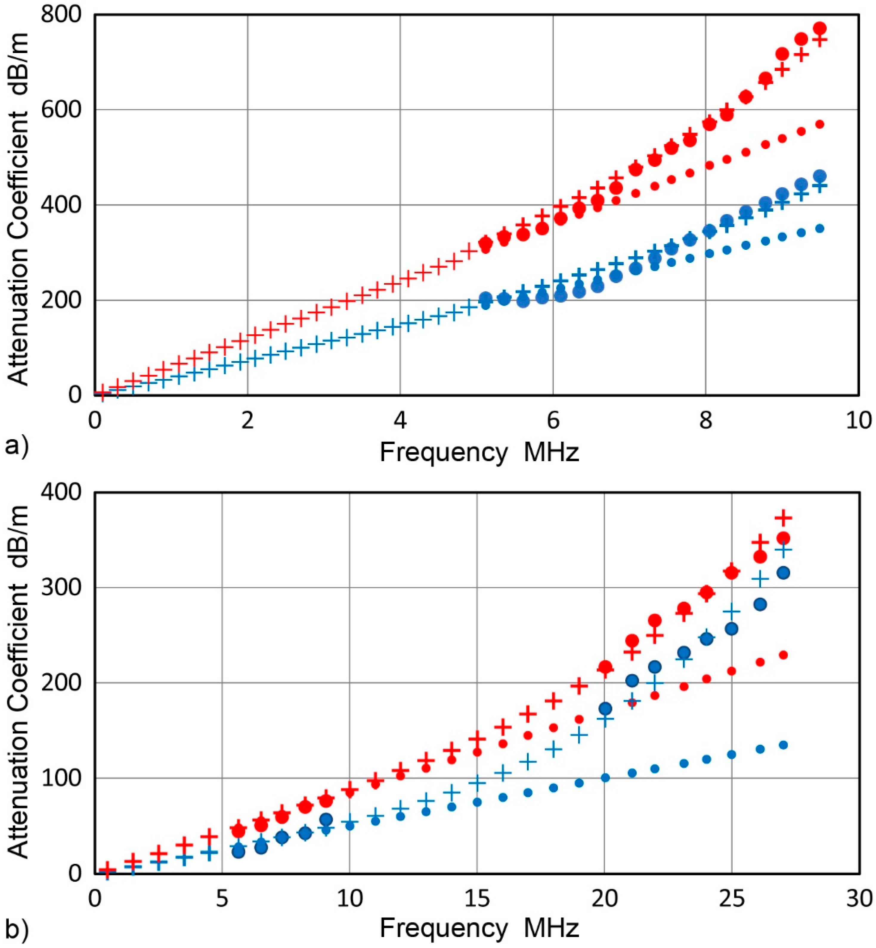
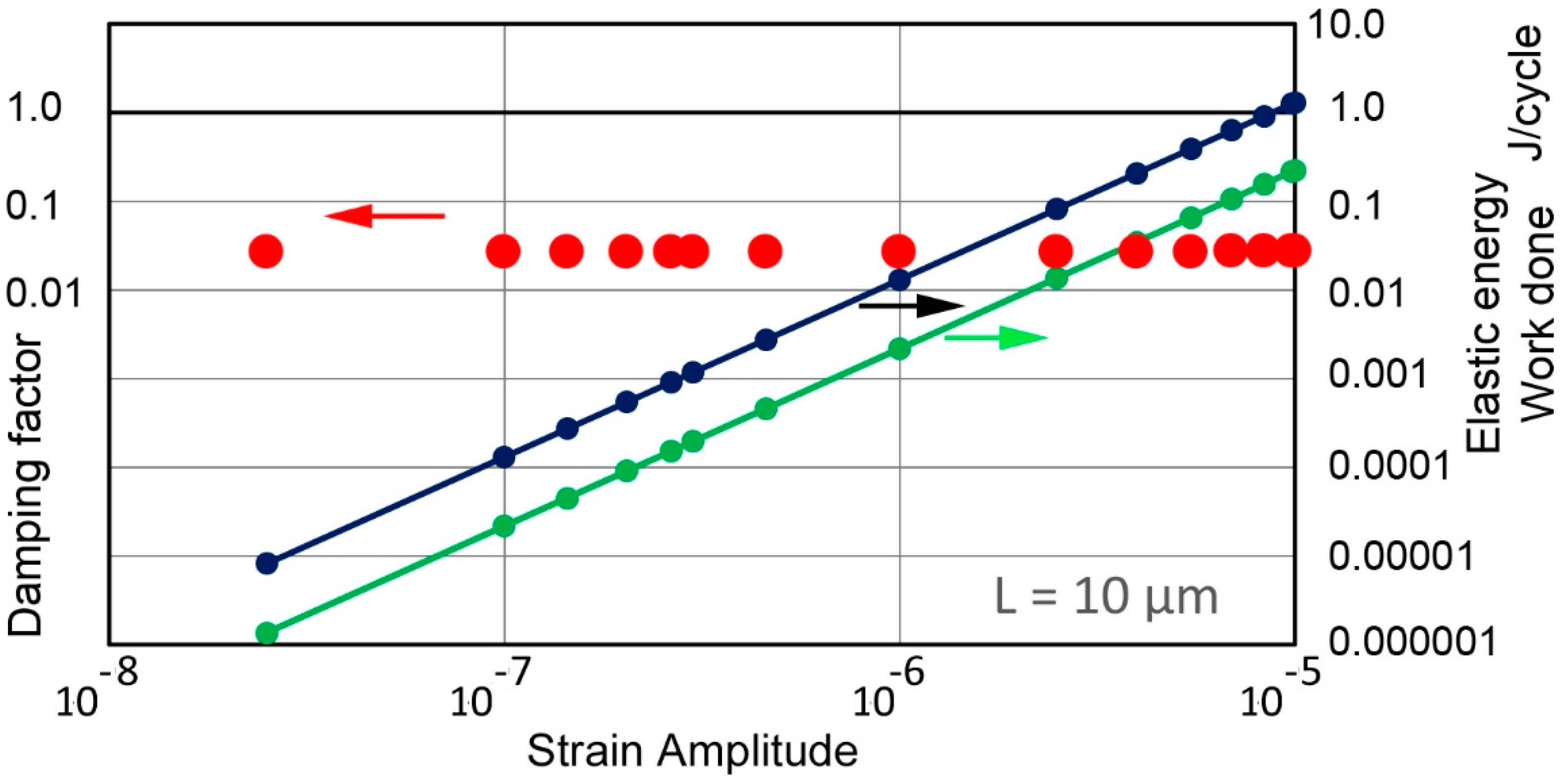
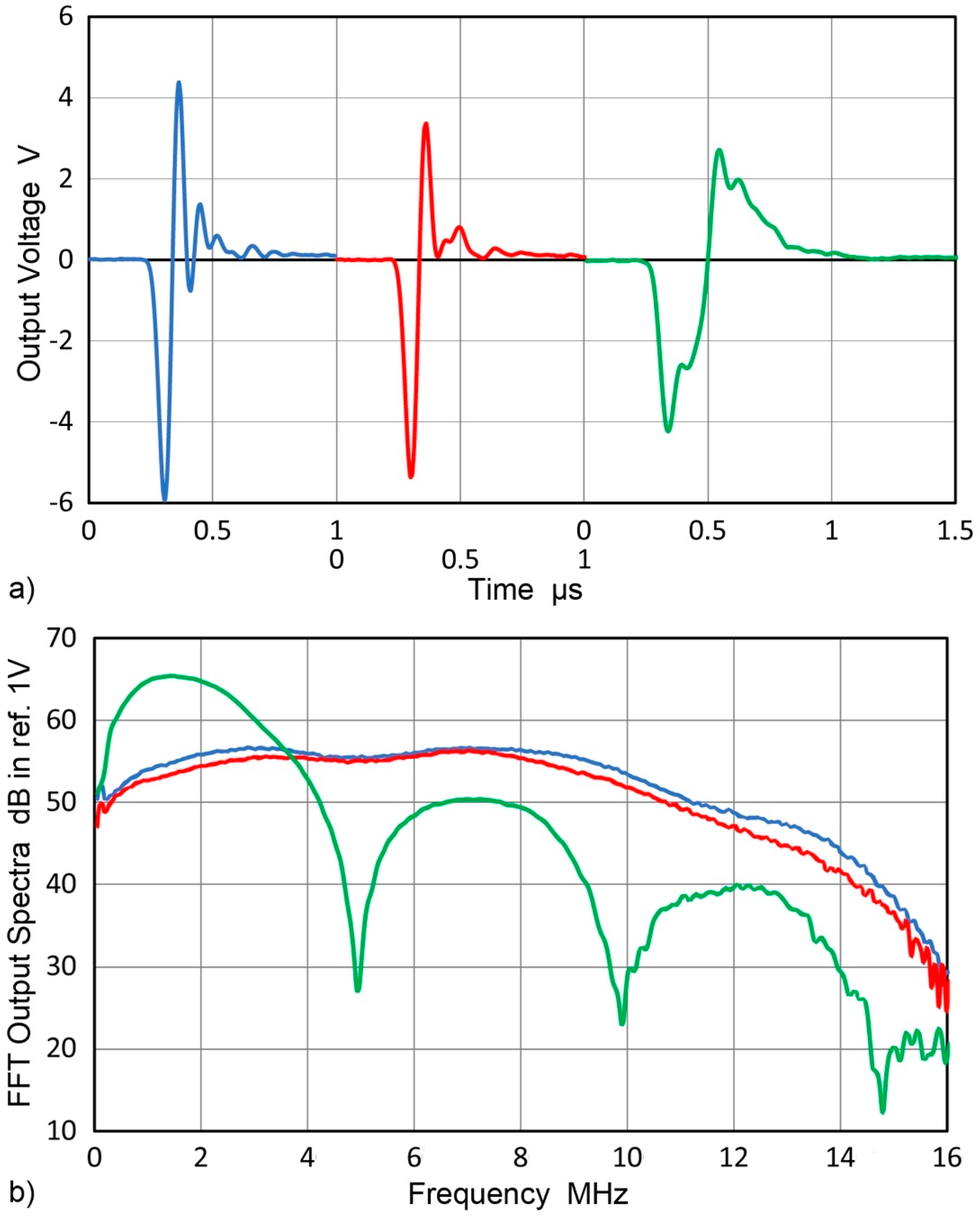
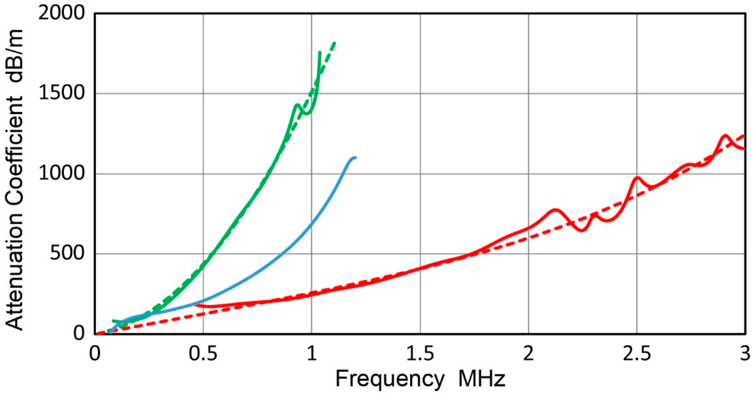6. Conclusions

Using contact ultrasonic measurement methods, it is possible to determine the attenuation characteristics of solid materials. The present methods only require commonly available UT instruments. Results from over 300 tests revealed various attenuation behaviors that were previously hidden because of the difficulty of obtaining reliable attenuation data. While plausible interpretation of some findings was possible by invoking a new dislocation damping mechanism, as well as Datta–Kinra and Biwa scattering, this study has demonstrated the need for further studies to correlate ultrasonic attenuation to nm-scale atomic motion.