CFD-Based Metamodeling of the Propagation Distribution of Styrene Spilled from a Ship

Abstract

The present study aimed to numerically establish a new metamodel for predicting the propagation distribution of styrene, which is one of the hazardous and noxious substances (HNSs) spilled from ships. Three-dimensional computational fluid dynamics (CFD) simulations were conducted for 80 different scenarios to gather large amounts of data on the spatial distribution of the change in concentration over time. We used the commercial code of ANSYS Fluent (V.17.2) to solve the Reynolds-averaged Navier–Stokes equations, together with the scalar transport equation. Based on the CFD results, we adopted the well-known kriging model to create a metamodel that estimated the propagation velocity and spatial distributions by considering the effect of the current surface velocity, deep current velocity, surface layer depth, and crack position. The results show that the metamodel accurately predicted the changes in the local distribution of styrene over time. This model was also evaluated using the hidden-point test.

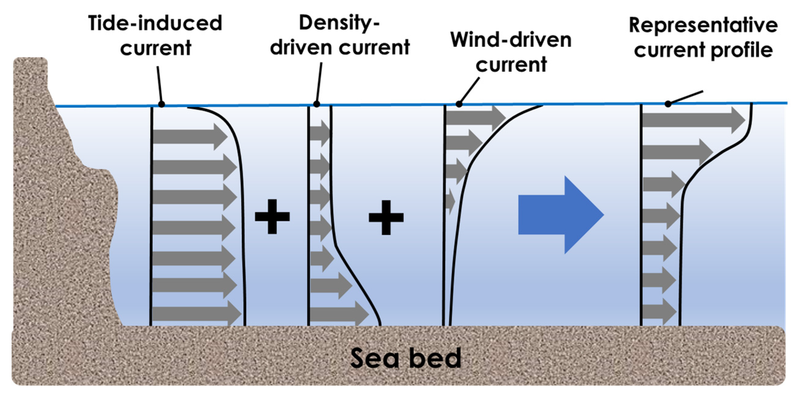
1. Introduction

Hazardous and noxious substances (HNSs), often transported by ships, are harmful to living resources, marine life, and even human health when spilled into the sea [1,2,3]. Because most HNSs, unlike oil, are transparent, the HNSs are difficult to recognize directly after leakage. In general, the HNS can be classified into gases (G), evaporates (E), floaters (F), dissolvers (D), and sinkers (S), as they float, evaporate, or dissolve [4]. For instance, the Ievoli Sun, a chemical tanker, sank in the English Channel and released approximately 4000 tons of styrene [5]. In this accident, high-intensity currents caused significant dilution, spreading styrene in the seawater, and styrene was detected in the gill tissues of crabs in the vicinity of the wreck. More than 2000 HNSs are being transported by ships currently; thus, a robust and quick response strategy for spill accidents should be developed.

According to the literature, there are many reports on oil spill problems. Can et al. [6] performed a numerical analysis of the leakage from an oil container ship in the Istanbul Strait and provided information on the oil propagation. Elhakeem et al. [7] developed a combined model using the hydrodynamic and oil-spill models. They also conducted a numerical simulation of the oil-spill propagation in the case of real accidents in the Arabian Gulf region, showing that the simulated results agreed well with the observed spill trajectories. As mentioned above, the oil spill was not difficult to visualize in the experiment because the oil was not transparent. However, because HNSs are optically transparent and very dangerous it is very difficult to conduct experiments in a real marine environment. Hence, many experimental works have been conducted in restricted areas and conditions. For example, Fuhrer et al. [8] released a floating cell containing a small amount of styrene into the sea and monitored the residual concentration over time. They reported that only 50% of the initial amount of spilled styrene remained just after one hour. Furthermore, experimental data have been reported in the Standard European Behavior Classification (SEBC) code. However, these data have limitations because the experiments were mostly conducted for pure products under atmospheric conditions in a laboratory. It turns out that these conditions significantly differ from those in the case of incidents at sea. Consequently, actual propagation behavior is different from the experimental results reported previously.

Another issue in carrying out the experiments is about the safety caused by the lethal toxicity of the HNSs. When the real experiment is conducted in the sea, the marine ecosystem and living resources will be at risk and eventually destroyed. Thus, doing a real experiment is strictly limited. Computational works are a promising alternative for the detailed investigation of HNS propagation behavior under various conditions. Even if the computational fluid dynamics (CFD) approach yields a lot of information on HNS propagation for various scenarios, it requires a huge amount of time to obtain the final solutions. Practically, we should make specific responses as quickly as possible just after HNS spill accidents. In this regard, CFD simulation cannot be used practically; however, a direct prediction tool, such as a metamodel, can be a powerful way to suggest how to respond to the HNS accident quickly.

Indeed, the metamodel is a surrogate model, which includes the mathematical relationship between inputs and outputs [9,10,11]. To develop the metamodel, we needed to gather a lot of information on the related physics. Hence, the present study extensively conducted CFD simulations for different cases and it suggested important parameters that can be used to mathematically connect inputs and outputs. Previously, a regression model was reported and tested with the CFD simulation results [12,13]. The current study aimed to construct the metamodel with the simulation results for 80 scenarios. Styrene was used as the HNS material and the propagation behavior of styrene in the sea was predicted in detail over a 360° degree range with 10° degree interval. This study also considered the representative current-velocity profile expressed in terms of surface current velocity (v_s), deep current velocity (v_d), and depth of the surface layer (d_s). Moreover, the hidden point tests were conducted to obtain more accurate solutions.

2. Mathematical Representations

2.1. Kriging Model

The metamodel can be efficient and practical for the quick prediction of HNS propagation without further CFD simulations, contributing to a rapid response after an accident [14]. The present study simulated a total of 80 cases and used the well-known kriging model to develop the meta-model [14,15]. According to the kriging model, we first set the unknown function y(x) consisting of a regression model and the stochastic process:

$$y\left(x\right)=f\left(x\right)+Z\left(x\right)$$

(1)

where f(x) represents the approximation function, and Z(x) represents the localized deviation interpolating the n sampled values by considering a Gaussian distribution. A correlation between Z(x_i) and Z(x_j) is given by a covariance matrix of the samples as follows:

$$Cov\left[Z\left(x^i\right),Z\left(x^j\right)\right]={\sigma }^{2}R\left(\left[R\left(x^i,x^j\right)\right]\right),$$

(2)

where R is the correlation matrix, which is an (n × n) diagonal-symmetric matrix, and σ² is the process variance. R(x_i,x_j) represents the Gaussian correlation function, which is expressed as:

$$R\left(x_k^i,x_k^j\right)=\exp \left[-{{\displaystyle \sum }}_{i,j=1}^n{\theta }_k{\left|x_k^i-x_k^j\right|}^2\right].$$

(3)

The predictor can be described at an arbitrary point x using:

$$\stackrel{⌒}{y}=\stackrel{⌒}{\beta }+r^T\left(x\right)R^{-1}\left(y-f\stackrel{⌒}{\beta }\right)$$

(4)

where y is the CFD simulation results (a column vector of length n), and f is an n × 1 unit column vector. r^T(x) represents a column vector {x₁, ..., x_n} of arbitrary points x. This column vector is expressed as follows:

$$r^T\left(x\right)={\left[R\left(x_k,x_k^1\right),R\left(x_{k,}{x}_k^2\right),\cdot \cdot \cdot ,\hspace{0.17em}R\left(x_k,x_k^n\right)\right]}^T$$

(5)

In Equation (4), $\stackrel{⌒}{\beta }$ is mathematically given by ${\left(f^T{R}^{-1}f\right)}^{-1}{f}^T{R}^{-1}y$. The correlation parameter θ_k in Equation (3) is also determined using maximum likelihood estimation as follows:

$$\max \underset{{\theta }_k>0}{\mathsf{\Phi }}\left({\theta }_k\right)=-\left[n\ln \left({\stackrel{⌢}{\sigma }}^2\right)+\ln \left|R\right|\right]/2,$$

(6)

where ${\stackrel{⌒}{\sigma }}^2$ is estimated using:

$${\stackrel{⌒}{\sigma }}^2=\left[{\left(y-f\stackrel{⌒}{\beta }\right)}^T{R}^{-1}\left(y-f\stackrel{⌒}{\beta }\right)\right]/n.$$

(7)

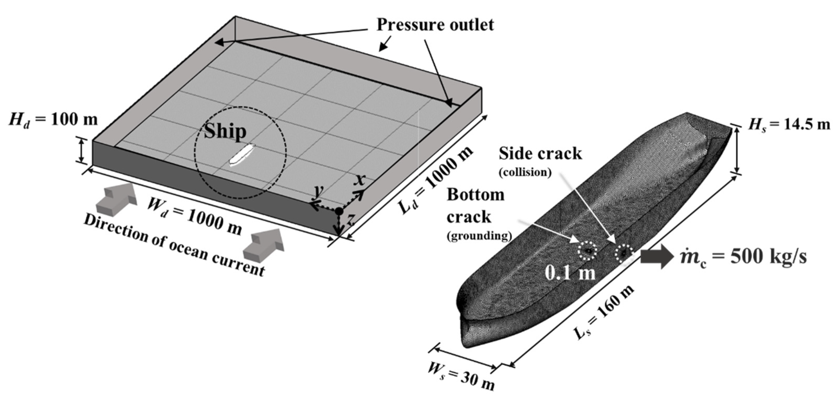
2.2. CFD Model

We needed a lot of data to develop the metamodel of the styrene propagation in the sea. Hence, the present study extensively conducted three-dimensional CFD simulations to obtain the predictions of the styrene concentration distribution by solving the Reynolds-averaged Navier–Stokes equations and the scalar transport equations at the same time. We used the commercial code of ANSYS Fluent (V.17.2) for simulations. Since the characteristic length is in the order of several hundred meters, the flow can be regarded as a turbulent flow around the ship. The present study adopted the standard k-ε model for simplicity. Numerically, we solved the mass and momentum conservation equations, which are expressed as follows:

$$\frac{\partial \rho }{\partial t}+\frac{\partial \left(\rho {\bar{u}}_i\right)}{\partial x_i}=0,$$

(8)

$$\frac{\partial }{\partial t}\left(\rho {\bar{u}}_i\right)+\frac{\partial }{\partial x_i}\left(\rho {\bar{u}}_i{\bar{u}}_j\right)=-\frac{\partial p}{\partial x_i}+\frac{\partial }{\partial x_i}\left[\mu \left(\frac{\partial {\bar{u}}_i}{\partial x_j}+\frac{\partial {\bar{u}}_j}{\partial x_i}-\frac{2}{3}{\delta }_{ij}\frac{\partial {\bar{u}}_l}{\partial x_l}\right)\right]+\frac{\partial }{\partial x_j}\left(-\rho u_i^{\prime }{u}_j^{\prime }\right),$$

(9)

where ρ denotes density, u_i denotes the velocity vector, and μ denotes viscosity. The present simulation used the standard k-ε model, and the wall function to predict turbulent stresses at the wall in the simulation [16]. The standard k-ε model can be expressed as:

$$\frac{\partial }{\partial t}\left(\rho k\right)+\frac{\partial }{\partial x_i}\left(\rho {\bar{u}}_{i}k\right)=\frac{\partial }{\partial x_j}\left[\left(\mu +\frac{{\mu }_t}{{\sigma }_k}\right)\frac{\partial k}{\partial x_j}\right]+G_k+G_b-\rho \epsilon ,$$

(10)

$$\frac{\partial }{\partial t}\left(\rho \epsilon \right)+\frac{\partial }{\partial x_i}\left(\rho {\bar{u}}_i\epsilon \right)=\frac{\partial }{\partial x_j}\left[\left(\mu +\frac{{\mu }_t}{{\sigma }_{\epsilon }}\right)\frac{\partial \epsilon }{\partial x_j}\right]+C_1\frac{\epsilon }{k}\left(G_k+G_b\right)-C_2\rho \frac{{\epsilon }^2}{k},$$

(11)

$${\mu }_t=C_{\mu }\rho \frac{k^2}{\epsilon },$$

(12)

where k and ε represent the turbulent kinetic energy and the dissipation rate, respectively. Furthermore, μ_t denotes the turbulent viscosity and G_k denotes the production of turbulent kinetic energy due to the mean shear rates. Here, G_b indicates the turbulent kinetic energy production due to buoyancy. The model constants C₁, C₂, and C_μ were set to C₁ = 1.22, C₂ = 1.92, and C_μ = 0.09. The turbulent Prandtl numbers were set to Pr_k = 1.0 and Pr_ε= 1.3. The species transport equation was adopted to describe the convection–diffusion for the kth species as follows:

$$\frac{\partial }{\partial t}\left(\rho Y_k\right)+\frac{\partial \left(\rho {\bar{u}}_i{Y}_k\right)}{\partial x_i}=-\frac{\partial J_{jk}}{\partial x_j},$$

(13)

where J_jk and Y_k are the diffusion flux and the mass fraction of species k, respectively.

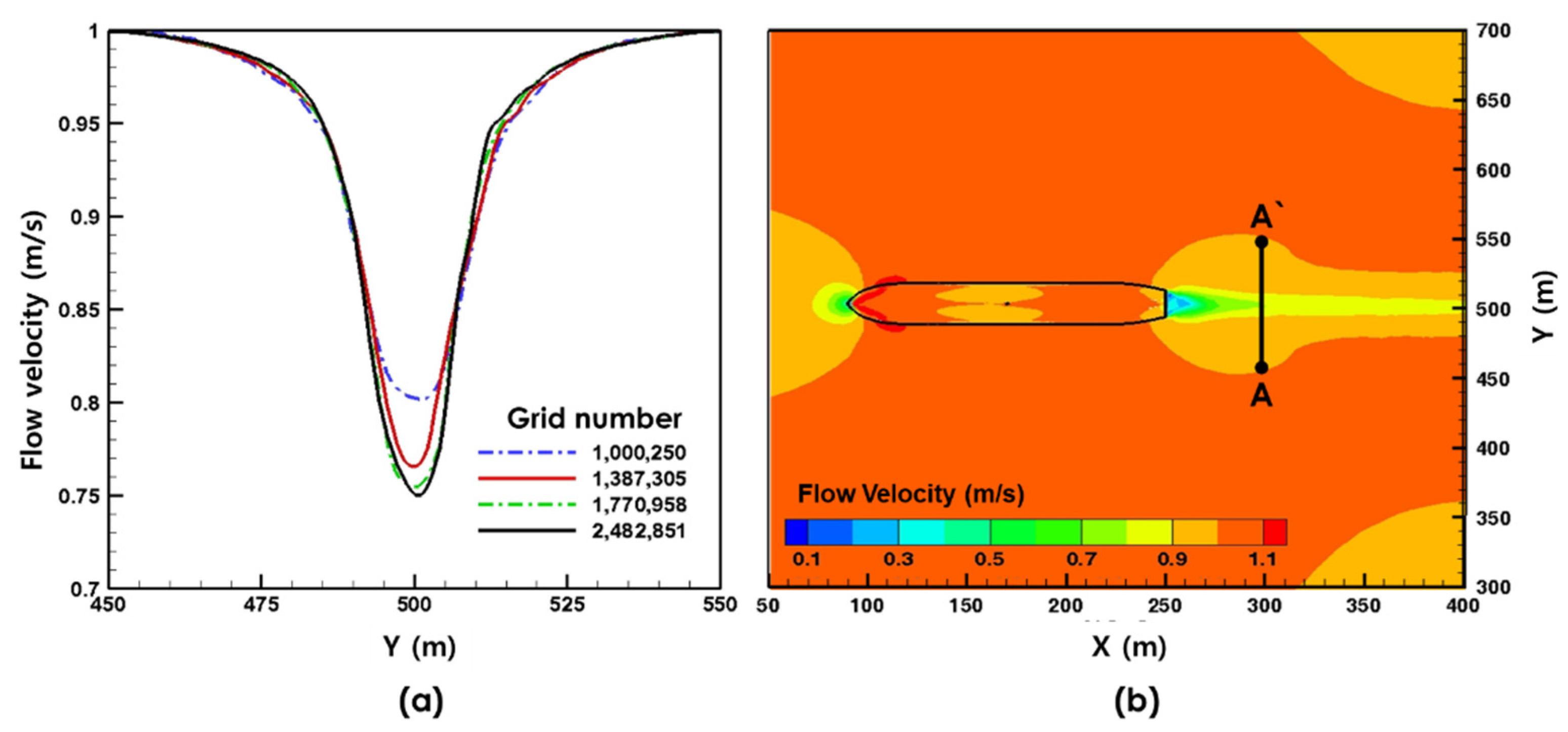
2.3. Numerical Details

Among various HNSs, the present study used a styrene material for the simulation based on knowledge of detailed scenarios with various current–velocity conditions. Figure 1 shows the schematic of the model that represents the current-velocity profile. It is known that the current-velocity profile consists of a tide-induced current, a density-driven current, and a wind-driven current [17,18]. Because of the complexity of atmospheric conditions, we modeled the current-velocity profile in terms of the surface current velocity (v_s), deep current velocity (v_d), and depth of surface layer (d_s). The present study considered four parameters, as follows: i) the surface velocity (v_s), ii) the ratio of the deep current velocity to surface current velocity (v_d/v_s), iii) the depth of the surface layer (d_s), and iv) the crack positions as the side (collision) and bottom (grounding). The surface velocity was set in the range from 0.1 to 1 m/s, and the deep current velocity was taken to be 30% to 100% of the surface current velocity (v_s). Furthermore, the depth of the surface layer was in the range of 10 to 100 m. The simulation conditions were finally set for 80 cases. The present simulation ignored the interfacial waves between the seawater and air for simplicity because it would have required tremendous computational resources and complicated data about atmospheric conditions. Hence, the slip condition at sea level was taken as the boundary condition. Furthermore, the pressure out condition was used for all surfaces except for the bottom surface, upon which the wall boundary condition was applied. The density, viscosity, and diffusivity properties of styrene were set to 906 (kg/m³), 0.76 × 10⁻³ (kg/(m∙s)) and 2.0 × 10⁻⁹ (m²/s), respectively. It was also important to establish the accident scenario. This simulation was conducted under the scenarios considering two cracks from the side (collision) and bottom (grounding) [19,20]. Based on information provided by KRISO (Korea Research Institute of Ships & Ocean Engineering), a mass flow rate from a crack was set as 500 kg/s. With a time step of 0.05 s, the transient simulation was performed for a total simulation time of 1000 s. The corresponding averaged Courant number was estimated to be 0.1231, and the maximum Courant number of 0.9232 was found near the crack position. The estimated y⁺ values were in the range of 100 to 220, showing an acceptable range for predicting turbulent stresses appropriately.

As shown in Figure 2, the computational domain had a size of 1000 m × 1000 m × 100 m. The detailed configuration of the ship was provided by KRISO. The accident ship had a length of 160 m, a width of 30 m, and a draft of 14.5 m. The crack with its area of 0.25 m² was positioned at 80 m from the front of the ship. Furthermore, another scenario considered a side crack that could form owing to collision-induced damage. The side-crack was located at 10 m below sea level, and the bottom crack due to grounding was located at the center of the bottom surface of the ship. We used the tetrahedral grid system and built much finer grids around the ship, as shown in Figure 2b. For the grid convergence test, we compared the velocity profile behind the ship (x = 290, z = 0, 450 m < y < 550 m) in the case of v_s = 1, v_d/v_s = 0.5, and d_s = 30 m. As shown Figure 3a, the maximum deviation between grid numbers of 1,770,958 and 2,482,851 was estimated to be 0.7% at y = 500 m. Therefore, the present study adopted 1,770,958 elements and 322,925 nodes after the grid convergence tests. We set the convergence criterion for the continuity as 10⁻⁴, for the energy as 10⁻⁶, and for others as 10⁻³.

3. Results and Discussion

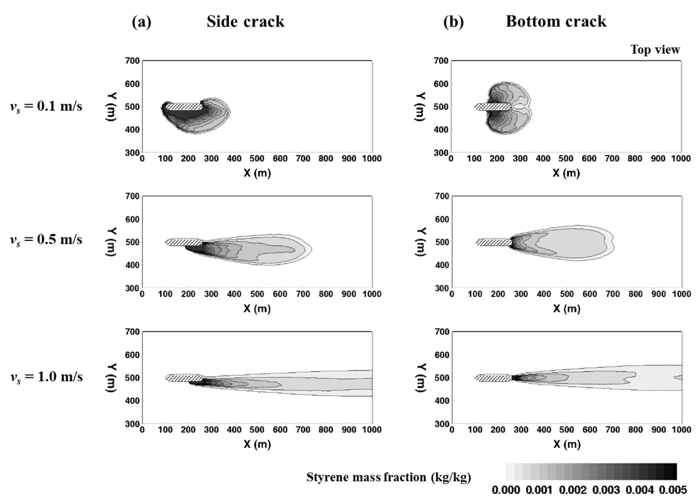
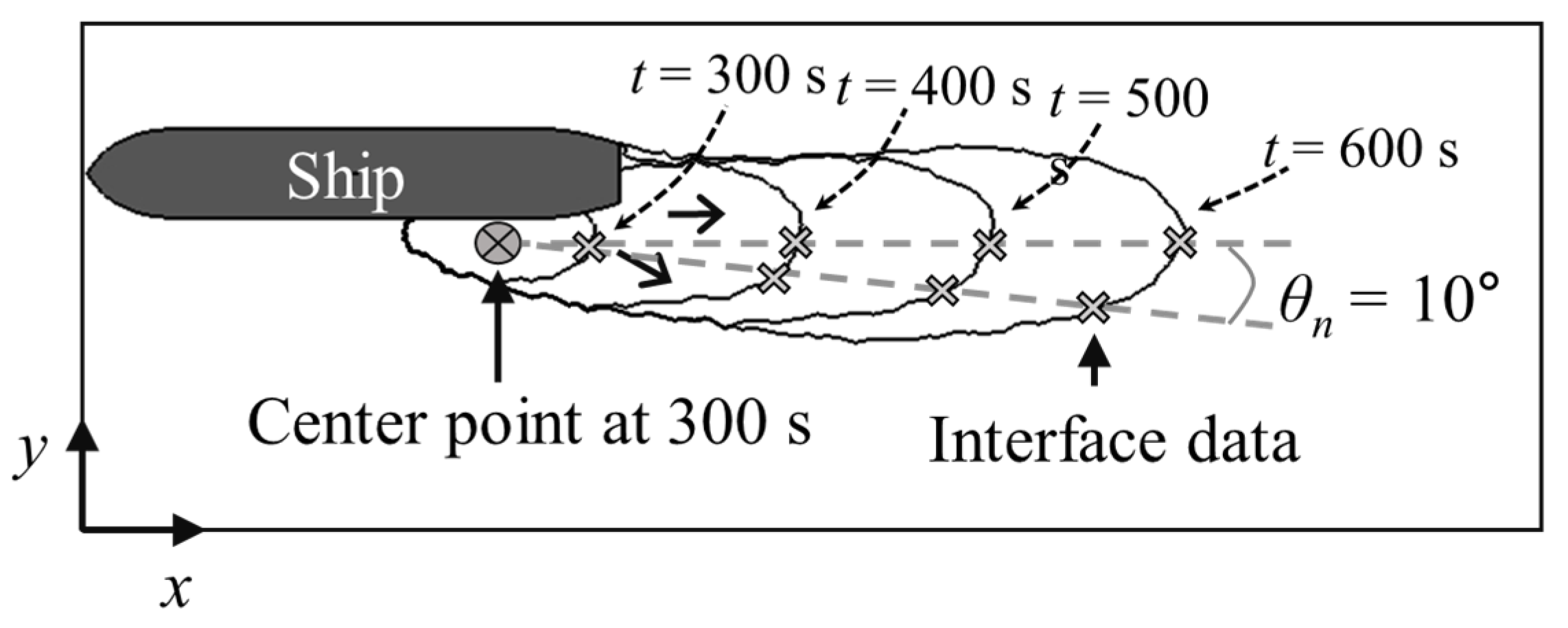
3.1. Propagation Characteristics

Figure 4a,b presents the predicted propagation behavior of styrene with different current velocities at a flow time 1000 s after leaking began. As expected, the surface current velocity (v_s) substantially affects the diffusive characteristics of styrene propagation. As the surface current velocity increased, styrene propagated much faster owing to the advection effect, whereas the styrene propagation was barely affected by the crack positions. The latter was because styrene, as a floating material, rapidly moved upward after being spilled from the crack, indicating the propagation behaviors at the side and bottom cracks were almost the same. Unlike the bottom crack, the styrene distribution in the side crack case showed a slightly asymmetric shape. After considering three factors, namely the surface current velocity, deep current velocity, and surface layer depth, it was found that the surface current velocity significantly affected the propagation behavior after a styrene spill.

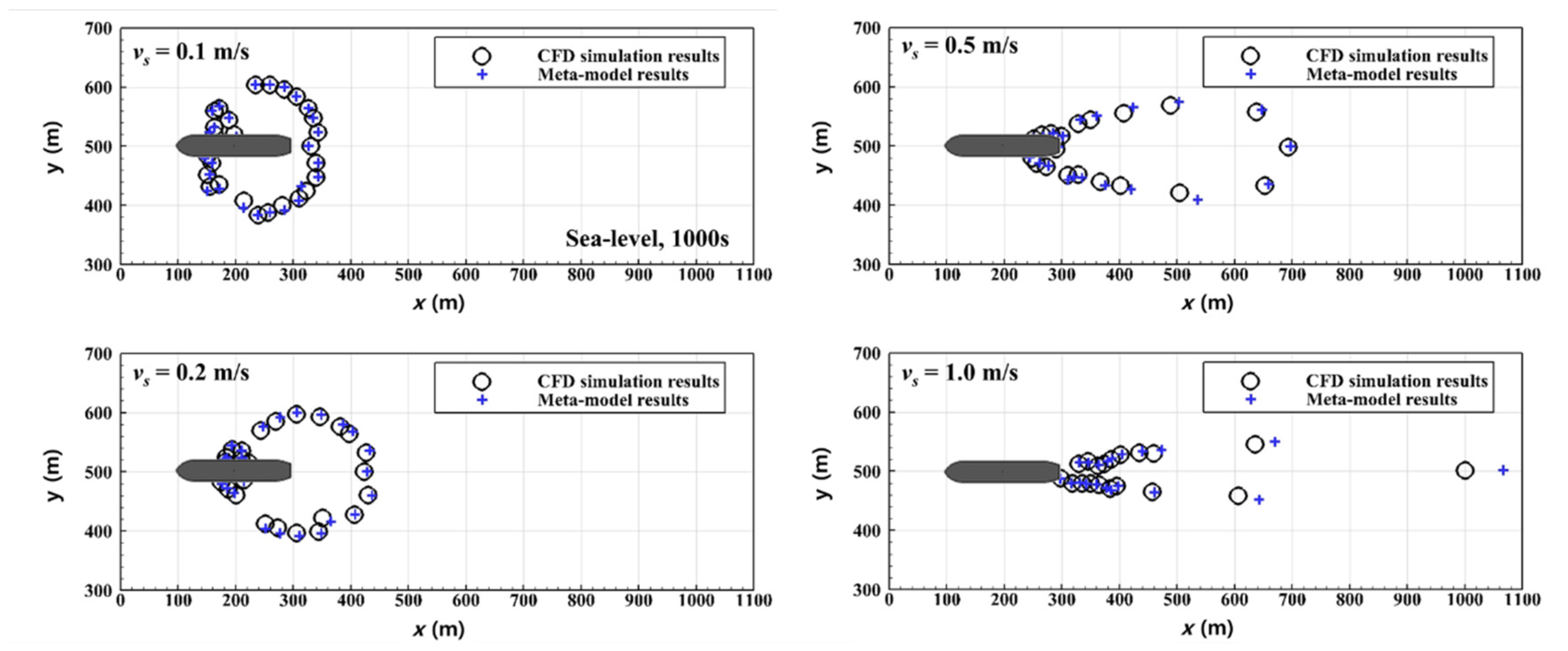
3.2. Estimation of Styrene Distribution

As stated above, saving time costs and getting accurate solutions are the ultimate objectives of metamodeling. Hence, we numerically simulated 80 cases and stored the acquired data for different variables, such as local velocity, kinetic energy, pressure, concentration, and so on. A metamodel connects inputs (scenario) and outputs (prediction) mathematically. Thus, we need to find out new parameters that are useful for responding to an accident. The present study suggested two parameters, as illustrated in Figure 5, which were the change in propagation distribution with time and the propagation velocity of the styrene interface.

First, the two parameters were estimated from the CFD results, and then those parameters were implemented in the kriging model. In Figure 5, a criterion regarding styrene concentration was taken as 100 ppm, corresponding to the exposure limit of styrene specified by the Occupational Safety and Health Administration [21]. Based on this criterion, the propagation velocity of styrene interface could be calculated as follows: first, the center point was selected as a middle point of the styrene interface at t = 300 s after the spill, and the interface area was then divided into intervals of 10° based on the center point, as shown in Figure 5. At a certain time, a two-dimensional interface contour line and the lines formed every 10° intersected each other at some points; the propagation velocity of the styrene interface and the propagation distribution were then estimated at these points. Finally, all data successively stored with time were used to make the metamodel.

Figure 6 shows the predicted styrene interface location at t = 1000 s according to the surface current velocity, which was predicted using the present metamodel in the bottom crack case with v_d/v_s = 0.5 and d_s = 30 m. The blue dot represents the styrene interface. It shows that at a low surface current velocity, the diffusion effect became dominant, and the styrene interface had an almost circular shape. As the surface current velocity increased, the shape of the styrene interface was closer to an ellipse due to the large advection effect. The goodness of fit was evaluated using R² and RMSE (root mean square error). As listed in

Table 1. The summary of fit with using R² and RMSE.

Vs (m/s)	Vd/Vs	Ds (m)	Lc	R2	RMSE
0.1	0.5	30	Bottom	0.9773	2.17
0.2	0.5	30	Bottom	0.9335	6.43
0.5	0.5	30	Bottom	0.9575	6.91
1.0	0.5	30	Bottom	0.9494	12.83

, the R² values were greater than 0.9, which means that the metamodel provided a good fit.

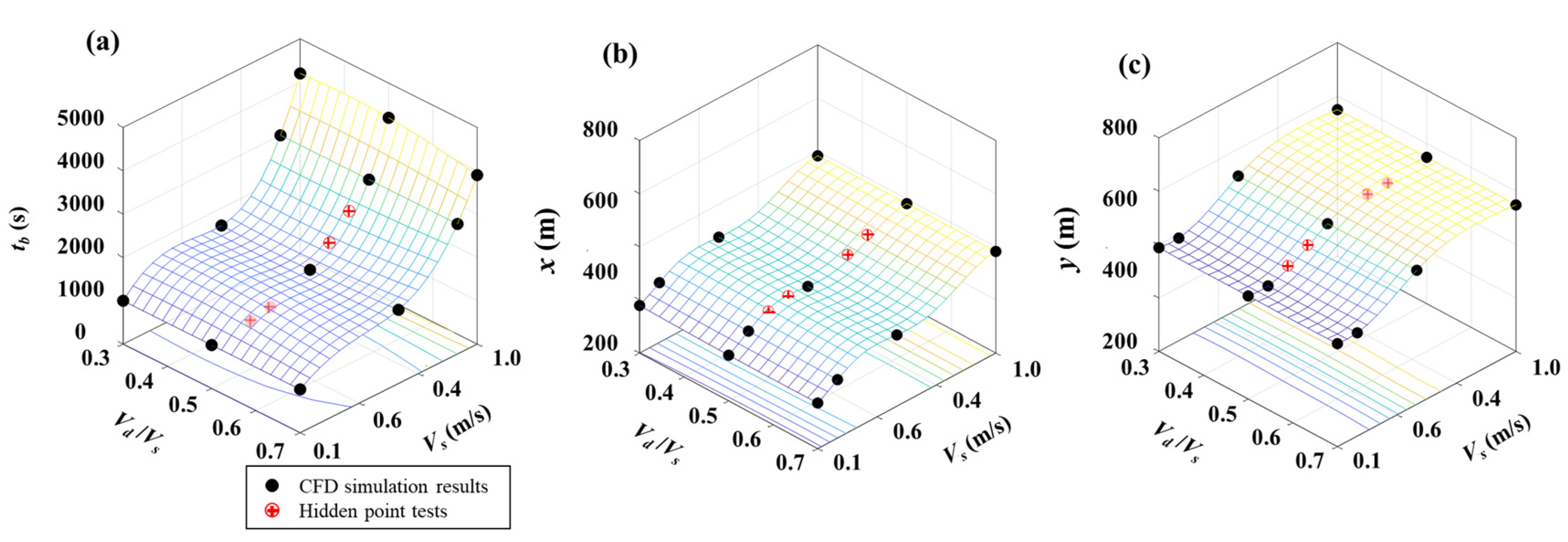
3.3. Hidden-Point Tests for the Evaluation

Mostly, comparison with experimental data has been widely adopted for model evaluation in many relevant numerical studies. Unfortunately, there is no available data for direct comparison of styrene under the specified conditions. Instead, we used another method, the so-called hidden point (or layer) method, which has been mainly introduced in machine learning and neural networks. More clearly, the hidden point (or condition) is not included in 80 different CFD cases that are used in making the current metamodel. Hidden points are new scenarios. Based on them, the CFD simulation was first conducted and then the metamodel ran separately, and finally, the two results were compared. We also selected three additional parameters, the first of which was the boundary arrival time t_b, defined as a time at which the styrene interface reached the outmost boundary face of the computational domain. The two other parameters were the x and y coordinates of the styrene interface at t = 1000 s after the spill started. Figure 7 shows the contours calculated by the metamodel at the given D_s of 30 m in the case of a bottom crack. The surface represents the response of the metamodel for the inputs, the black dot represents the CFD simulation result from 80 cases taken in the present study, and the red dot indicates the metamodel prediction based on the hidden point.

The comparison result is summarized in

Table 2. Eight additional cases for the hidden-point test and the corresponding errors of the metamodel for the boundary arrival time (t_b).

Case No.	Vs (m/s)	Vd/Vs	Ds (m)	Lc	δ1 (%)	δ2 (%)
Case 1	0.30	0.5	30	Side	12.3	9.2
Case 2	0.30	0.5	30	Bottom	12.1	7.3
Case 3	0.40	0.5	30	Side	11.0	6.4
Case 4	0.40	0.5	30	Bottom	12.1	5.1
Case 5	0.70	0.5	30	Side	19.6	4.8
Case 6	0.70	0.5	30	Bottom	37.4	5.6
Case 7	0.80	0.5	30	Side	37.8	3.7
Case 8	0.80	0.5	30	Bottom	46.6	4.7

. The CFD simulations were performed for eight additional cases, which were regarded as the hidden points. Those eight cases are listed in Table 2 were not included in the 80 cases used for making the metamodel. For measuring the relative error between the CFD result and the metamodel prediction, the quantitative error of boundary arrival time could be estimated using:

$${\delta }_1=\frac{V^{\prime }-V}{V}\times 100\hspace{0.17em}(\%)$$

(14)

where V’ denotes the metamodel prediction at the hidden point and V represents the CFD result at the same point. For the x- and y-coordinates of the styrene interface, the relative error was obtained using:

$${\delta }_2=\frac{{\displaystyle \sum _{i=1}^3{\displaystyle \sum _{j=1}^{36}{\displaystyle \sum _{k=1}^{42}\left(\frac{V^{\prime }-V}{V}\times 100\right)}}}}{i\cdot j\cdot k}(\%)$$

(15)

where i denotes the coordinate, and j and k represent the angle and the time, respectively. The estimated error of the styrene interface was less than 9.2%, which shows a relatively good performance. As shown in Table 2, the created metamodel showed relatively good for qualitatively predicting how the spatial distribution changed with time, though it provided a big difference and showed a low accuracy.

The kriging method is a kind of inverse distance weighted (IDW) method. It uses the interpolation by giving larger weights to the adjacent points. Therefore, the accuracy of the metamodel can be increased by extending the database. To improve the accuracy of the metamodel for predicting the boundary arrival time, four cases (3, 4, 6, and 7) were selected and put into the previous database for 80 cases. Then, with the newly updated database with 84 cases, the metamodel could be updated by calculating the coefficients again with the use of Equation (4). For the evaluation, we compared the results of the modified metamodel with the CFD results for the hidden point cases 1, 2, 5, and 6.

Table 3. Error analysis for the modified metamodel.

Case No.	δ1 (%)
Case 1	5.0
Case 2	4.0
Case 5	9.7
Case 6	11.8

shows the relative errors for the modified metamodel, which shows a better performance at predicting the boundary arrival time. For instance, the 37.4% error for case 6 was reduced to 11.8%. This model will be updated continuously by performing further simulations for additional cases to enhance the model’s performance.

4. Conclusions

The present study developed a new metamodel for predicting the styrene propagation distribution and boundary arrival time. Two important parameters were introduced and the extensive CFD simulations were carried out. A mathematical relationship between inputs and outputs was established using the kriging model. To feed the big data that were necessary to make the metamodel, the present study extensively conducted three-dimensional transient CFD simulations for 80 different cases from the taken scenarios. The following conclusions were drawn.

The present study presented the CFD simulation results and analyzed the influence of current profiles on the propagation characteristics. Due to the floating behavior of styrene, the concentration fields were concentrated near the sea level and the interface of styrene moved much faster in the streamwise direction as the surface velocity increased. This was clearly because the advection effect became dominant and most of the styrene propagated near the sea’s surface.

• A new metamodel was provided to estimate the propagation distribution and the boundary arrival time. Based on CFD results, the main parameters were calculated and implemented in the metamodel. A comparison was made between CFD results and the metamodel prediction, showing good agreement between them. This verified that the current model could predict the transient characteristics of styrene propagation well. Thus, the use of the metamodel would be a powerful tool for the quick estimation of HNS propagation that can be used to formulate a fast response in the early stages after accidents.
• This metamodel was evaluated using the hidden point tests. By adding data from eight additional cases, the performance of the metamodel was improved. For instance, a 37.4% error was reduced to 11.8% due to the modification. Thus, the current model will be updated continuously to achieve better accuracy via modification with additional data from further CFD simulations.

References

- IMO. Protocol on preparedness, Response and co-operation to pollution incidents by hazardous and noxious substances. 2000 (OPRC-HNS Protocol); IMO: London, UK, 2000. [Google Scholar]
- Neuparth, T.; Moreira, S.; Santos, M.M.; Reis-Henriques, M.A. Hazardous and noxious substances (HNS) in the marine environment: Prioritizing HNS that pose major risk in a european context. Mar. Pollut. Bull. 2011, 62, 21–28. [Google Scholar] [CrossRef] [PubMed]
- Harold, P.D.; De Souza, A.S.; Louchart, P.; Russell, D.; Brunt, H. Development of a risk-based prioritisation methodology to in-form public health emergency planning and preparedness in case of accidental spill at sea of hazardous and noxious substances (HNS). Environ. Int. 2014, 72, 157–163. [Google Scholar] [CrossRef] [PubMed]
- Bonn Agreement, Counter pollution manual. Bonn Agreemment Counter Pollution Manual. 1991. Available online: https://www.bonnagreement.org/publications.
- Law, R.J.; Kelly, C.; Matthiessen, P.; Aldridge, J. The loss of the chemical tanker Ievoli Sun in the English Channel, October 2000. Mar. Pollut. Bull. 2003, 46, 254–257. [Google Scholar] [CrossRef]
- Can, S.; Celik, F.; Yilmaz, H.; Bak, O.A. Oil spill simulation: A case study in the strait of Istanbul. Fresenius Environ. Bull. 2007, 16, 1517–1522. [Google Scholar]
- Elhakeem, A.A.; Elshorbagy, W.; Chebbi, R. Oil spill simulation and validation in the Arabian (Persian) Gulf with special reference to the UAE coast. Water Air Soil Pollut. 2007, 184, 243–254. [Google Scholar] [CrossRef]
- Fuhrer, M.; Peron, O.; Hofer, T.; Morrissette, M.; Le Floch, S. Offshore experiments on styrene spillage in marine waters for risk assessment. Mar. Pollut. Bull. 2012, 64, 1367–1374. [Google Scholar] [CrossRef]
- Wen, J.; Yang, H.Z.; Jian, G.P.; Tong, X.; Li, K.; Wang, S.M. Energy and cost optimization of shell and tube heat exchanger with helical baffles using kriging metamodel based on MOGA. Int. J. Heat Mass Tranf. 2016, 98, 29–39. [Google Scholar] [CrossRef]
- Rulik, S.; Wroblewski, W.; Fraczek, D. Metamodel-based optimization of the Labyrinth Seal. Arch. Mech. Eng. 2017, 64, 75–91. [Google Scholar] [CrossRef]
- Mao, X.F.; Zhang, W.X.; Qian, J.K.; Wu, M.H. CFD based multi-disciplinary optimization design of high performance deep sea seismic vessel. In Proceedings of the ASME 36th International Conference on Ocean, Offshore and Arctic Engineering, Trondheim, Norway, 25–30 June 2017; p. 1. [Google Scholar]
- Jeong, C.H.; Ko, M.K.; Lee, M.; Lee, S.H. Numerical simulation of propagation characteristics of hazardous noxious substances spilled from transport ships. Appl. Sci. 2018, 8, 2409. [Google Scholar] [CrossRef]
- Ko, M.K.; Jeong, C.H.; Lee, M.; Lee, S.H. Development of a metamodel for predicting near-field propagation of hazardous and noxious substances spilled from a ship. Appl. Sci. 2019, 9, 3838. [Google Scholar] [CrossRef]
- Simpson, T.W.; Mistree, F. Kriging models for global approximation in simulation-based multidisciplinary design optimization. AIAA J. 2001, 39, 2233–2241. [Google Scholar] [CrossRef]
- Wahba, G. Spline Models for Observational Data (CBMS-NSF Regional Conference Series in Applied Mathematics); Society for Industrial and Applied Mathematics: Philadelphia, PA, USA, 1990; p. 169. [Google Scholar]
- Launder, B.E.; Spalding, D.B. The numerical computation of turbulent flows. Comput. Methods Appl. Mech. Eng. 1974, 3, 269–289. [Google Scholar] [CrossRef]
- Sellar, B.G.; Wakelam, G.; Sutherland, D.R.J.; Ingram, D.M.; Venugopal, V. Characterisation of tidal flows at the European marine energy center in the absence of ocean waves. Energies 2018, 11, 176. [Google Scholar] [CrossRef]
- Samolyubov, B.I.; Ivanova, I.N. The evolution of velocity profiles and turbulent viscosity in a system of currents with wind-induced and density flows. Mosc. Univ. Phys. Bull. 2014, 69, 426–432. [Google Scholar] [CrossRef]
- Ventikos, N.P.; Papanikolaou, A.D.; Louzis, K.; Koimtzoglou, A. Statistical analysis and critical review of navigational accidents in adverse weather conditions. Ocean Eng. 2018, 163, 502–517. [Google Scholar] [CrossRef]
- Friis-Hansen, P.; Simonsen, B.C. GRACAT: Software for grounding and collision risk analysis. Mar. Struct. 2002, 15, 383–401. [Google Scholar] [CrossRef]
- Occupational Safety and Health Administration, OSHA Occupational Chemical Database. 2018. Available online: https://www.osha.gov/chemicaldata/chemResult.html?recNo=14 (accessed on 18 December 2018).