Prediction of Weights during Growth Stages of Onion Using Agricultural Data Analysis Method

Abstract

In this study, we propose a new agricultural data analysis method that can predict the weight during the growth stages of the field onion using a functional regression model. We have used onion weight on growth stages as the response variable and six environmental factors such as average temperature, average ground temperature, rainfall, wind speed, sunshine, and humidity as the explanatory variables in the functional regression model. We then define a least minimum integral squared residual (LMISE) measure to obtain an estimate of the function regression coefficient. In addition, a principal component regression analysis was applied to derive the estimates that minimize the defined measures. Next, to evaluate the performance of the proposed model, data were collected, and the following results were identified through analyses of the collected data. First, through graphical and correlation analysis, the ground temperature, mean temperature, and humidity have a very significant effect on the onion weights, but environmental factors such as wind speed, sunshine, and rainfall have a small negative effect on onion weights. Second, through functional regression analysis, we can determine that the ground temperature, sunshine, and precipitation have a significant effect on onion growth and are essential in the goodness-of-fit test. On the other hand, wind speed, mean temperature, and humidity did not significantly affect onion growth. In conclusion, to promote onion growth, the appropriate ground temperature and amount of sunshine are essential, the rainfall and the humidity must be low, and the appropriate wind or mean temperature must be maintained.

1. Introduction

In general, onions produced in various parts of Korea are highly value-added vegetables, as they are used not only for various dishes but also as part of a healthy diet. Therefore, farmers who cultivate vegetables in the field are concerned with cultivation strategies that can improve the vegetable yields. In addition, the related agencies, such as the Rural Development Administration, devote much attention to developing onion cultivation techniques to address the farmers’ needs [1].

However, the onion growth among vegetables is especially affected by the change of weather. In general, onions have the characteristic of being well grown in low temperature and dry weather. Because of this characteristic, if rainy weather prevails, onion yields drop significantly, whereas onion yields increase considerably in predominantly sunny weather. Therefore, if onion production is excessively increased, onion prices will drop, whereas prices will be excessively high if production is low. For this reason, maintaining an appropriate level of production in government offices and farms is vital.

Hence, we are going to examine how the production of onion grown in the field is affected by various weather conditions and environmental factors and try to develop the best farming strategy based on them. To get the right answers to these problems, we first examine both the mathematical theory and application of the functional regression model, which is the most suitable statistical model for analyzing time series data collected directly from the agricultural field. Second, on the basis of onion data collected from various regions, we examine the effects of various environmental factors and climatic conditions on the onion yields using the functional regression model. Finally, we would like to propose an optimal farming strategy that can maintain appropriate levels of the various environmental factors and weather.

2. Related Works

Yields of crops or vegetables are predicted using various statistical data analysis models, pattern recognition methods, and deep learning algorithms. First, Kamilaries and Prenafeta-Boldu [2] conducted a survey of more than 40 previous studies for artificial intelligence technologies applied to various agricultural and crop production problems. They looked at the specific agricultural problems under study, the particular models and systems used, and the data correction and pretreatment. They also reviewed the overall performance of each study. Furthermore, they compare the artificial intelligence method with other existing popular technologies, such as various machine learning methods and statistical prediction models. Second, Manikandan and Vethamoni [3], in their review paper, proposed how agricultural statistical techniques can be used to define the ordering of researches and to understand the elementary interactions among plant soil atmospheric elements. As a research tool, developing and applying models can contribute to more efficient and targeted research planning. Third, Bhange and colleagues [4] wrote a paper that suggests ways to help farmers choose the optimal conditions for their farm, depending on various environmental and soil factors such as temperature, humidity, water level, soil type, soil PH, fertilizer, and cultivated interval or season factors. They have carried out this prediction using a random forest classification machine learning algorithm. Fourth, Mythra and colleagues [5] presented a brief comparative study of several papers discussing various techniques used to determine crop yields. This paper determined the appropriate data processing model to realize high accuracy and prediction ability. Fifth, Sekkam and Poovammal [6] analyze environmental factors such as cultivated area, annual rainfall, and food price index that affect crop yields and relate the relationships to these factors. In this study, multiple regression analysis was used to analyze environmental factors and their impact on crop yields. Sixth, Abdelkhalik and colleagues [7] conducted field experiments on two farming stages in Spain to evaluate how effective controlled deficit different irrigation water facilities are for onion growth and total yields. They found that deficit irrigation strategies have reduced marketable yields. Hence, if enough water is available, full irrigation is recommended. Seventh, Maskey and colleagues [8] published a paper exploring the correlation of various environmental factors affecting the yields of strawberries grown in an open field. In addition, they use the principal component regression method, two pattern recognition techniques such as a one-layer neural network model, and the random forest classification method to evaluate yield prediction. The weather parameters used in this study are a combination of sensor data obtained in strawberry fields, weather data observed from a nearby weather station, and agricultural sources such as cooling time. Eighth, Rathod and Mishra [9] used both linear and nonlinear as well as parametric and nonparametric statistical models to predict the yields of Karnataka’s mangoes and bananas. They proposed a hybrid model consisting of linear and nonlinear models. This model, consisting of a combination of autoregressive integrated moving average (ARIMA) and support vector machine regression (SVMR), performed better than other researchers’ methods in terms of validity and verifiability of the model. Ninth, Villiers [10] has written a master’s thesis on the topic of predicting the tomato yields from weather data using machine learning technology. In his master’s thesis, he found that all crops and weather variables are beneficial for predicting tomato yield. Furthermore, for the most important prediction of the median, mean, and total yield density, he considered the daily average wind speed and the maximum daily relative humidity during the growing season of each crop.

3. Dataset and Method

3.1. Dataset

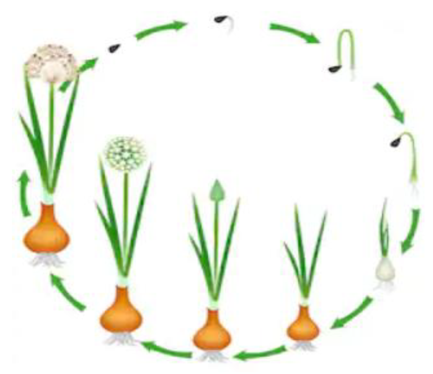
Here we are going to consider how to grow onions, which are popular among Koreans and used in various dishes, to improve onion growth. Generally, onions are sown in mid-August to mid-September, planted quite early in October to early November, and harvested between May and June of the following year. Figure 1 shows the onion growing step by step [11].

Figure 1. Onion growing states in the cultivation process.

In this study, we used datasets of the various environmental factors and the weights of onion during growth stages collected from farmers in several regions of Korea from March 2019 to June 2019. We used six factors such as mean wind speed, mean temperature, mean ground temperature, mean humidity, daily sunshine, and daily rainfall as the explanatory variables of the model, and the onion weight growth stage was used as a response variable. A description of each variable is given in Table 1 below.

Table 1. The response variable and environmental variables used in data set.

Role	Variable Name	Unit of Measure
Response variable	Onion weight	g/one unit
Six environmental variables	Mean wind speed	mps
	Mean temperature	°C
	Mean ground temperature	°C
	Mean humidity	%
	Daily sunshine	$\mathrm{J}/{\mathrm{cm}}^2$
	Daily rainfall	mm

We collected a total of 178 observations from 28 farms and used them in the experiment. During the observation period, environmental factor data were used from the meteorological office data observed by region, and the onion weight was obtained from the measurements by the staff of the RDA (Rural Development Administration). Of the data collected from 28 farms, a total of 63 observations, repeated 9 times in 7 farms with relatively good measurements were used in the experiment. Here, each environmental variable was measured for 7 days and repeated for 9 weeks. Onion weight was measured 9 times from 7 farms during the same period. Finally, the data of environmental factors consisted of data obtained from measuring six factors through nine repeated measurements each week for 7 days for 7 objects. Therefore, the environmental factors are given in the form of a $64\times 35$ matrix. In addition, data on onion weights were obtained from nine replicate measurements of 7 farms. Thus, onion weight data is given in a matrix of $9\times 7$. Table 2 and Table 3 below show some part of the data on average wind speed among the six environmental factors as well as onion weight observed during the growth period.

Table 2. Example of input data of environmental variables of growth period.

var2 (t-7)	var3 (t-7)	var4 (t-7)	var5 (t-7)	var6 (t-7)	var7 (t-7)	var2 (t-1)	var3 (t-1)	var4 (t-1)	var5 (t-1)	var6 (t-1)	var7 (t-1)
1.4	12.5	12.4	43.8	11.6	0	1.3	16	16.9	59.6	5.4	0
1.2	13.3	16.5	45.5	11.5	0	2.1	13	16	42.3	11	0
1.2	14.8	19.5	53.1	11.5	0	1.7	11.8	13.8	86.4	0	10.5
1.6	10.6	12.8	87.5	0	56.5	1.7	17	22.3	54.1	11.9	0
1.2	16.1	18.7	84.9	0.7	32	1.2	20.2	23.3	70.4	7.2	2
1.1	18.5	22.4	74.5	1.3	0	1.2	16.1	18.7	84.9	0.7	32
1.2	20.4	24.3	62.1	11.6	0	2.5	14.8	20.1	56.8	7.3	0
1.8	16.3	22.4	66.4	2.5	0	1.1	21.2	26.2	61.3	4.7	0
1.4	21.2	28	71	7.8	0	1.4	23.9	31.9	53.5	10	0
1.4	12.5	12.4	43.8	11.6	0	1.3	16	16.9	59.6	5.4	0
1.2	13.3	16.5	45.5	11.5	0	2.1	13	16	42.3	11	0
1.2	14.8	19.5	53.1	11.5	0	1.7	11.8	13.8	86.4	0	10.5
1.6	10.6	12.8	87.5	0	56.5	1.7	17	22.3	54.1	11.9	0
1.1	18.5	22.4	74.5	1.3	0	1.2	16.1	18.7	84.9	0.7	32
1.2	16.1	18.7	84.9	0.7	32	1.2	20.2	23.3	70.4	7.2	2
1.2	20.4	24.3	62.1	11.6	0	2.5	14.8	20.1	56.8	7.3	0
1.8	16.3	22.4	66.4	2.5	0	1.1	21.2	26.2	61.3	4.7	0

Table 3. Example of input data of onion weight of growth period.

	farm1	farm2	farm3	farm4	farm5	farm6	farm7
week8	24.724	39.583	25.433	37.5	27.792	11.733	56.533
week9	72.067	98.375	67.067	87.767	74.75	38.133	134.2
week10	109.27	162.71	108.82	177.75	113.92	69.626	217.97
week11	124.2	196.33	154.97	210.73	149.42	102.2	242.07
week12	169.47	273.13	219.8	315.93	179.04	150.7	332.7
week13	203.03	312.88	244.13	364.77	216.25	153.37	371.52
week14	255.62	365.46	256.2	367.3	224.03	168.15	383.07
week15	257.3	395.73	279.3	405.03	224.79	192.63	389.3
week16	292.7	403.75	314.4	467.7	225.65	193.67	415.17

3.2. Method

We considered a functional sequence regression model with $p$ functional covariates to determine how $p$ environmental factors influence onion weights $n$ over time [12,13,14]. This model is defined as follows:

$$y_i\left(t\right)=\alpha \left(t\right)+{{\displaystyle \sum }}_{k=1}^p{{\displaystyle \sum }}_{s=1}^q{\beta }_k\left(s,t\right)x_{ik}\left(s\right) +{ϵ}_i\left(t\right),i=1,\cdots ,n$$

(1)

where $n$ is the number of observations, $p$ is the number of functional covariates, $y_i\left(t\right)$ is onion weight in time $t$, $x_{ik}\left(s\right)$ is the functional covariate, $\mathsf{\alpha }\left(t\right)$ is the mean functional, ${\beta }_k\left(s,t\right)$ is the regression functional for the $k$–th covariate, and ${ϵ}_i\left(t\right)$ is a random error function.

In this case, to derive the estimators of the function sequence parameter ${\beta }_k\left(s,t\right)$ of the proposed model, we use a criterion of the least minimum integral squared residual (LMISE) defined as:

$$\mathrm{LMISE}={\left|\left|\mathrm{y}-\widehat{y}\right|\right|}^2={{\displaystyle \sum }}_{i=1}^n{{\displaystyle \int }}_{{\mathcal{T}}_Y}^{}[y_i\left(t\right)-(\alpha \left(t\right)+{{{\displaystyle \sum }}_{k=1}^p{{\displaystyle \sum }}_{s=1}^q{x}_{ik}\left(s\right){\beta }_k\left(s,t\right))]}^{2}dt.$$

(2)

Here, we have applied the functional principal component analysis to obtain estimators of the functional regression parameters that can minimize the LMISE measure defined on above. In this case, we center the explanatory variables $x_{ik}$ and response variable $y_i$ as follows to remove the $\mathsf{\alpha }\left(t\right)$-intercept term of the model given in (1) above.

$$y_i^{*}\left(t\right)=y_i\left(\mathrm{t}\right)-\overline{y}\left(t\right), x_{ik}^{*}\left(s\right)=x_{ik}\left(s\right)-{\overline{x}}_k\left(s\right), k=1,\cdots ,p$$

(3)

First, we express the ${x_{ik}^{*}}^{\prime }s$ and $y_i^{*}$ in terms of finite sum using the basic functions ${{\varphi }_{jk}}^{\prime }s$ and ${\psi }_l$ as follows:

$$x_{ik}^{*}\left(s\right)={{\displaystyle \sum }}_{j=1}^J{c}_{ijk}{\varphi }_{jk}=c_{ik}^T{\varphi }_k, k=1,\cdots ,p,$$

(4)

and

$$y_i^{*}\left(t\right)={\displaystyle \sum }_{l=1}^L{d}_{il}{\psi }_l=d_i^T\psi$$

(5)

where $\varphi$ and $\psi$ are basis vector functions of size J and L, respectively. Furthermore, if we denote the coefficient matrix of these basis function vectors as ${\mathrm{C}}_k$ and $\mathrm{D}$, then we can write these expressions in the following matrix function form:

$${\mathrm{X}}_k^{*}={\mathrm{C}}_k\varphi , y^{*}=\mathrm{D}\psi .$$

(6)

Here, we can express the regression functional coefficient ${\beta }_k\left(s,t\right)$ as a double sum as expansion:

$${\beta }_k\left(s,t\right)={{\displaystyle \sum }}_{j=1}^J{{\displaystyle \sum }}_{l=1}^L{b}_{jlk}{\varphi }_{jk}\left(s\right){\psi }_l\left(t\right)={\varphi }_k^T\left(s\right){\mathrm{B}}_k\psi$$

(7)

where ${\mathrm{B}}_k$ is a $\left(J\times L\right)$ matrix of coefficients $b_{jlk}$, or, more compactly, as ${\beta }_k\left(s,t\right)={\varphi }_k^T{\mathrm{B}}_k\psi$.

We define ${\mathrm{J}}_{{\varphi }_k}$ and ${\mathrm{J}}_{\psi }$ as the matrices of inner products between the elements of the ${\varphi }_k$ and $\psi$ bases, respectively. Then, we have the following expression:

$${\mathrm{J}}_{{\varphi }_k}={{\displaystyle \int }}_{I_s}{\varphi }_k\left(s\right){\varphi }_k{\left(s\right)}^{T}ds, {\mathrm{J}}_{\psi }={{\displaystyle \int }}_{I_s}\psi \left(s\right)\psi {\left(s\right)}^{T}ds.$$

(8)

In addition, if we substitute, respectively, the sum expressions given in Equations (4) and (7) for $x_{ik}^{*}$ and ${\beta }_k$ in Equation (1), we can obtain:

$${\widehat{y}}^{*}\left(t\right)={{\displaystyle \sum }}_{k=1}^p{{\displaystyle \int }}_{I_s}^{}{\mathrm{C}}_k{\varphi }_k\left(s\right){\varphi }_k^T\left(s\right){\mathrm{B}}_k\psi \left(t\right)ds ={{\displaystyle \sum }}_{k=1}^p{\mathrm{C}}_k{\mathrm{J}}_{{\varphi }_k}{\mathrm{B}}_k\psi \left(t\right).$$

(9)

If we denote $\hat{\mathrm{D}}$ to be the matrix of coefficients of the basis expansion of the vector of predictors ${\widehat{y}}^{*}$ (corresponding to the matrix D for the vector $y^{*}$), we obtain the following matrix form for the estimated model:

$$\hat{\mathrm{D}}={{\displaystyle \sum }}_{k=1}^p{\mathrm{C}}_k{\mathrm{J}}_{{\varphi }_k}{\mathrm{B}}_k$$

(10)

Therefore, we can get a matrix form for the integrated squared residual:

$$\parallel {\widehat{y}}_i-y_i {\parallel }^2= \parallel {\widehat{y}}_i^{*}-y_i^{*} {\parallel }^2={\left(\left(\hat{\mathrm{D}}-\mathrm{D}\right){\mathrm{J}}_{\psi }{\left(\hat{\mathrm{D}}-\mathrm{D}\right)}^T\right)}_{ii}$$

(11)

and, finally, a criterion of the least minimum integral squared residual (LMISE)

$$\mathrm{LMISE}\left({\mathrm{B}}_k\right)= \mathrm{trace}\left(\left(\hat{\mathrm{D}}-\mathrm{D}\right){\mathrm{J}}_{\psi }{\left(\hat{\mathrm{D}}-\mathrm{D}\right)}^T\right)$$

(12)

is given by a sum of quadratic forms in the unknown coefficient matrices ${\mathrm{B}}_k$.

Furthermore, we are going to consider the minimization of the criterion LMISE $\left({\mathrm{B}}_k\right)$ given at Formula (12). In this case, if ${\mathrm{J}}_{{\varphi }_k}$ and ${\mathrm{J}}_{\psi }$ are identity matrices, and the matrix ${\mathrm{B}}_k$ will minimize the Formula (12) if and only if

$${\mathrm{C}}_k^T{\mathrm{C}}_k{\mathrm{B}}_k={ \mathrm{C}}_k^T\mathrm{D}$$

so that

$${\mathrm{B}}_k={\left({\mathrm{C}}_k^T{\mathrm{C}}_k\right)}^{-1}{\mathrm{C}}_k^T\mathrm{D}.$$

(13)

The matrix ${\mathrm{B}}_k$ is easily found by using the singular value decomposition (SVD) of ${\mathrm{C}}_k$. Here, we have obtained ${\mathrm{C}}_k={\mathrm{U}\mathsf{\Delta }}_{C_k}{\mathrm{V}}^T$, where ${\mathsf{\Delta }}_{C_k}$ is a diagonal matrix with strictly positive diagonal elements and $\mathrm{U}$ and $\mathrm{V}$ have orthogonal columns. Then,

$${\mathrm{C}}_k{}^T{\mathrm{C}}_k={\mathrm{V}\mathsf{\Delta }}_{C_k}^2{\mathrm{V}}^T,$$

(14)

and hence the Moore–Penrose g-inverse of ${\mathrm{C}}_k{}^T{\mathrm{C}}_k$ is ${\mathrm{V}\mathsf{\Delta }}_{C_k}^{-2}{\mathrm{V}}^T$. Substituting it into (13) gives us the following equation:

$${\mathrm{B}}_k={\mathrm{V}\mathsf{\Delta }}_{C_k}^{-1}{\mathrm{U}}^T\mathrm{D}$$

(15)

Therefore, if we substitute ${\mathrm{B}}_k$ into ${\beta }_k\left(s,t\right)$ in Equation (7), we get the following functional estimates for functional regression coefficients:

$${\widehat{\beta }}_k\left(s,t\right)={\varphi }_k^T\left(s,t\right){\hat{\mathrm{B}}}_k\psi$$

(16)

Finally, we can obtain the following predicted equation for response values:

$$\widehat{y}\left(t\right)=\overline{y}\left(t\right)+{{\displaystyle \sum }}_{k=1}^p{{\displaystyle \int }}_{I_s}{x}_{ik}\left(s\right){\widehat{\beta }}_k\left(s,t\right)ds$$

(17)

4. Experimental Results

4.1. Graphical Analysis

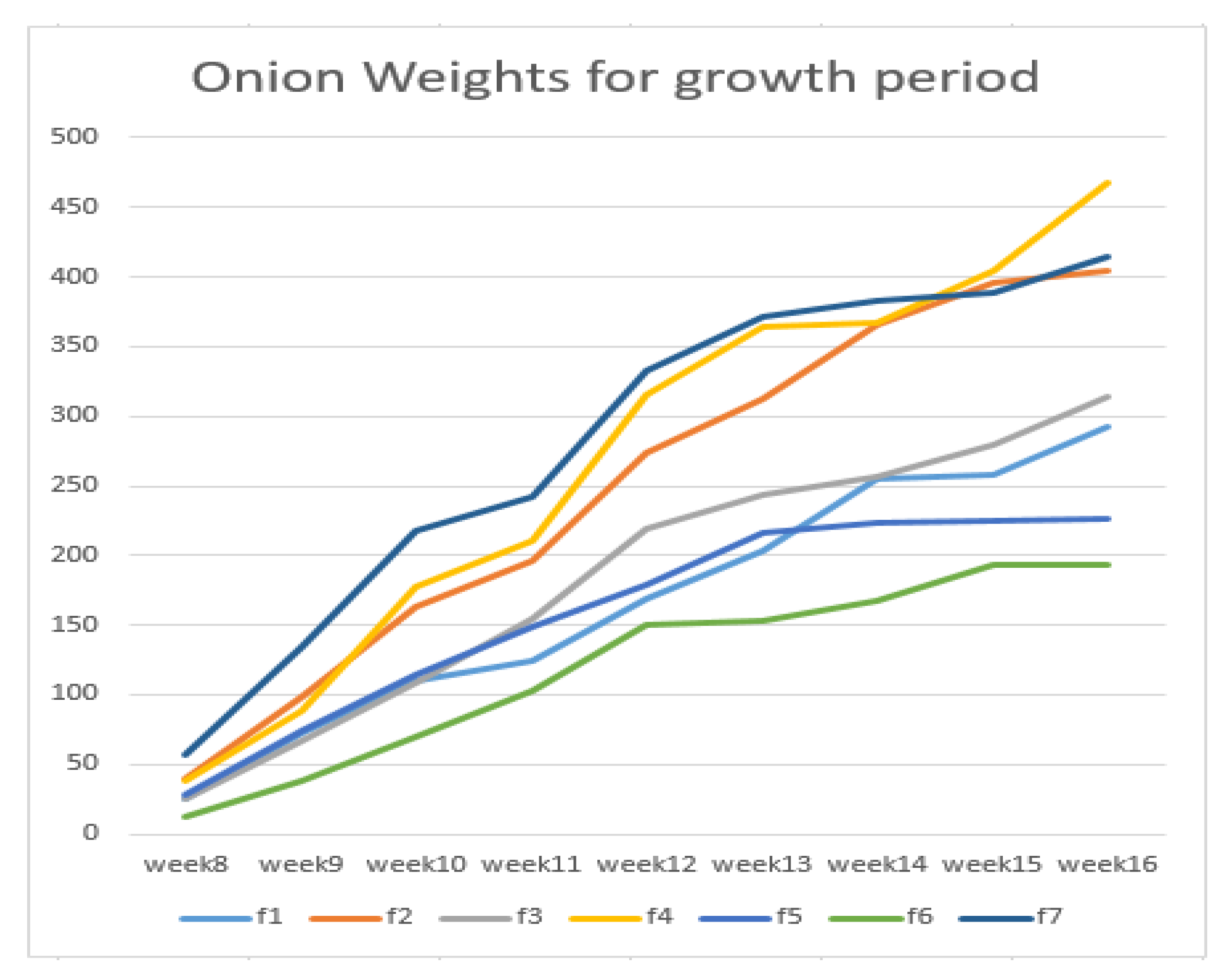
First, we plotted a line graph of the onion weights collected from seven farmers over nine weeks from transplantation to harvest. From Figure 2, we can see that the onion weight increases over time.

Figure 2. Line graphs of weight and six environmental factors.

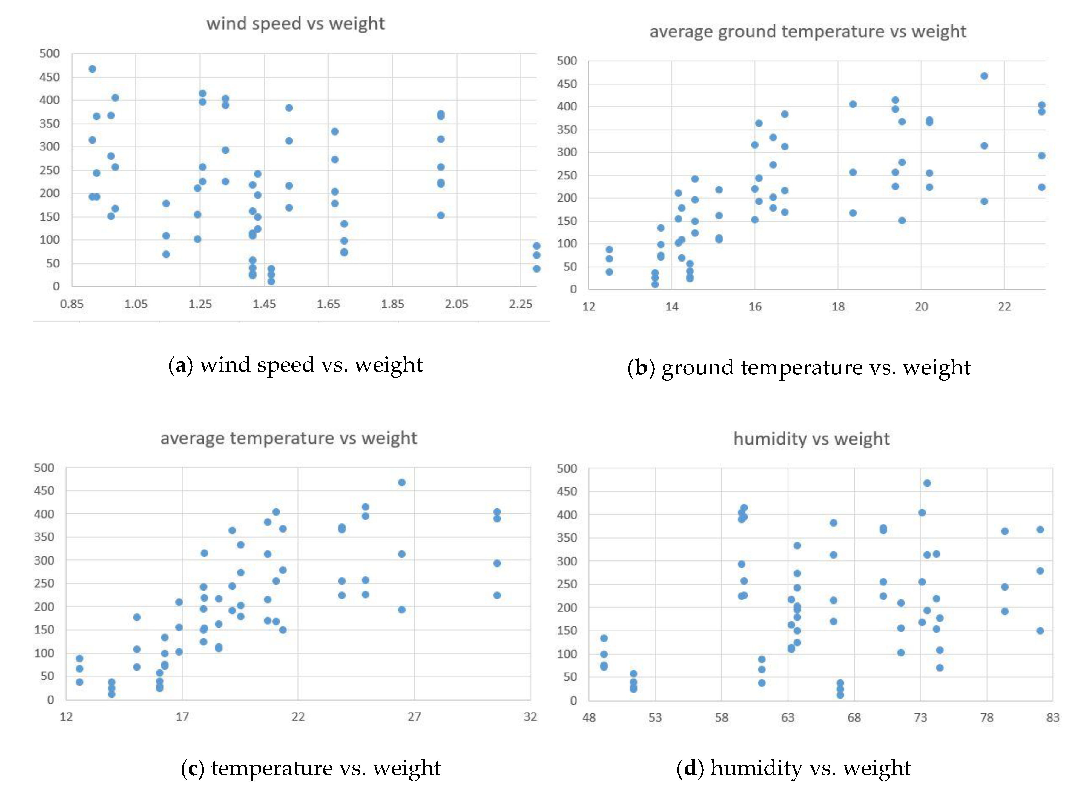
Second, a two-dimensional scatter plot was plotted to graphically determine the relationship between the onion weights and the mean of six environmental factors during the cultivated interval. Figure 3 shows the relationship between the onion weights and six environmental factors. As a result of Figure 3, we can see first that the average temperature and average ground temperature have a high positive correlation with the onion weights. It is evident that humidity has a small positive correlation with onion weight. Finally, three environmental variables such as wind speed, sunshine, and rainfall have no relation to onion weight.

Figure 3. Relationship between onion weights and six environmental factors.

Next, we calculated the correlation coefficient between each variable to statistically confirm the results derived so far. Table 4 shows the correlation coefficients between these variables. Given the results in Table 4, we can equally confirm the relationship between the variables discussed above.

Table 4. Correlation coefficients between onion weight and six environmental factors.

	Wind Speed	Ground Temp	Temp	Humidity	Sunshine	Rainfall	Weight
wind speed	1.00	−0.32	−0.31	−0.38	−0.26	0.02	−0.24
ground temp	−0.32	1.00	0.97	0.24	0.08	−0.51	0.73
temperature	−0.31	0.97	1.00	0.11	0.17	−0.41	0.73
humidity	−0.38	0.24	0.11	1.00	−0.53	0.17	0.34
sunshine	−0.26	0.08	0.17	−0.53	1.00	−0.35	−0.18
rainfall	0.02	−0.51	−0.41	0.17	−0.35	1.00	−0.11
weight	−0.24	0.73	0.73	0.34	−0.18	−0.11	1.00

4.2. Functional Data Analysis

We have applied a functional regression model with functional covariates and functional responses to see how the six environmental factors affect the onion weights over growing time. Here, to perform a functional data analysis on onion data, we have used the “fda” package in the R-software.

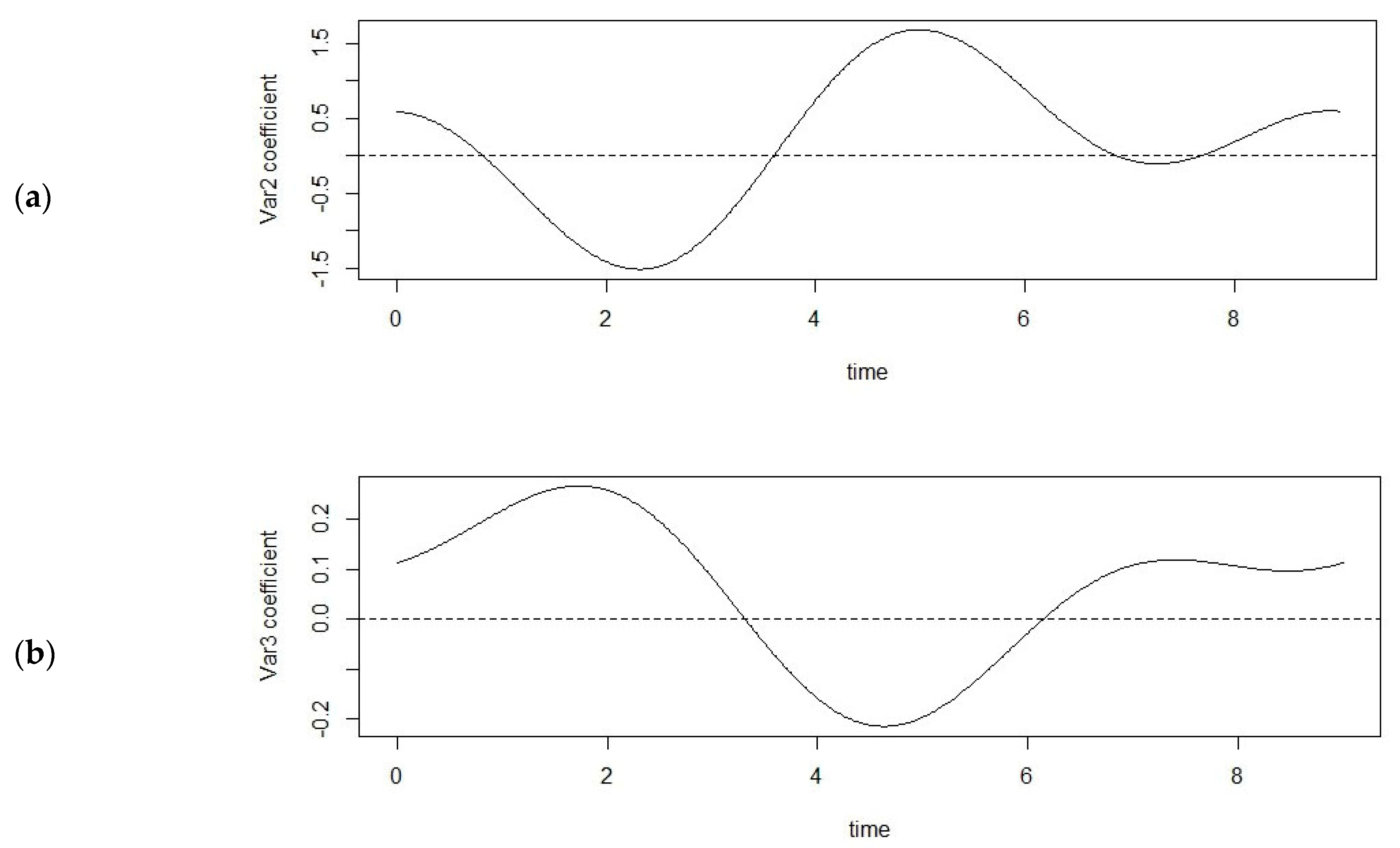
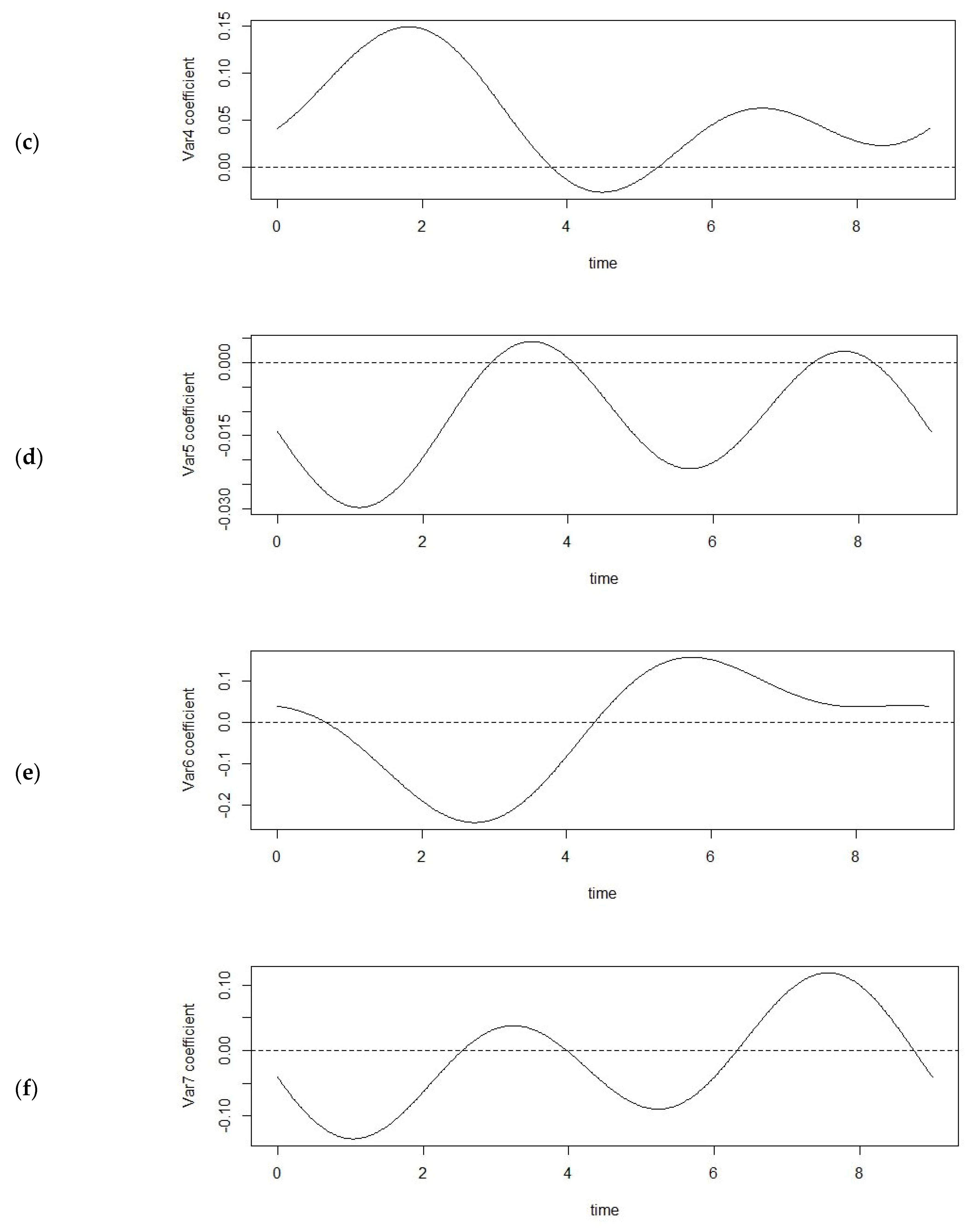
First, we conducted a functional data analysis to determine how six environmental variables influence the onion weights. Figure 4 shows the time series properties of the functional regression coefficients of each environmental factor during onion cultivation. In Figure 4, we first see that wind speed has a positive effect on the onion weights from the beginning to the middle, has a negative effect beyond the midpoint, and then has a positive effect again after the third quarter. Second, both the ground and mean temperature have a similarly positive effect in the early stage of onion weight growth, a negative effect at the midpoint, and a positive effect in the later growth period. Therefore, the ground temperature and average temperatures have a similar effect on onion radish growth, but the ground temperature has a relatively large magnitude in terms of influence. Third, humidity has a negative effect on onion weight throughout the growing season, but its impact is not significant. Fourth, the amount of sunshine has a positive effect early in the growth period of onions, a negative effect from the beginning to the middle, and a positive effect after the middle. Finally, rainfall has alternating positive and negative effects during onion growth, but its impact is not significant.

Figure 4. Regression coefficients in the prediction of onion weights from six environmental variables. (a) Wind speed, (b) mean temperature, (c) ground temperature, (d) humidity, (e) sunshine, (f) rainfall.

Second, we calculated the coefficients of determination ($R^2$) representing the explanatory power for the onion weights when environmental variables were used individually and when they were used together. We also calculated the F-test statistic to test the goodness-of-fit of each environmental variable for onion weight. Table 5 shows both coefficients of determination, $R^2$ represents the explanatory power of the onion weight for each environmental variable and the F-statistics used in the goodness-of-fit test. From Table 5 we can see that our results are similar to those above. We can also observe that if all environmental factors are used, the value of $R^2$ is the highest and the value of F-statistic is the largest. Additionally, individually, the value of $R^2$ and the F-statistic of ground temperature, sunshine, and rainfall is high. On the other hand, the value of $R^2$ and F-statistics of wind speed, mean temperature, and humidity are lower.

Table 5. Coefficients of determinations and F-statistics for six environmental factors.

Factors	Max (R2)	Mean (R2)	F-Statistic
wind speed	0.71	0.19	4.97
ground temp	0.46	0.2	5.3
temperature	0.46	0.13	4.87
humidity	0.27	0.11	4.53
sunshine	0.63	0.26	5.5
rainfall	0.49	0.33	5.75
All variables	0.94	0.83	29.36

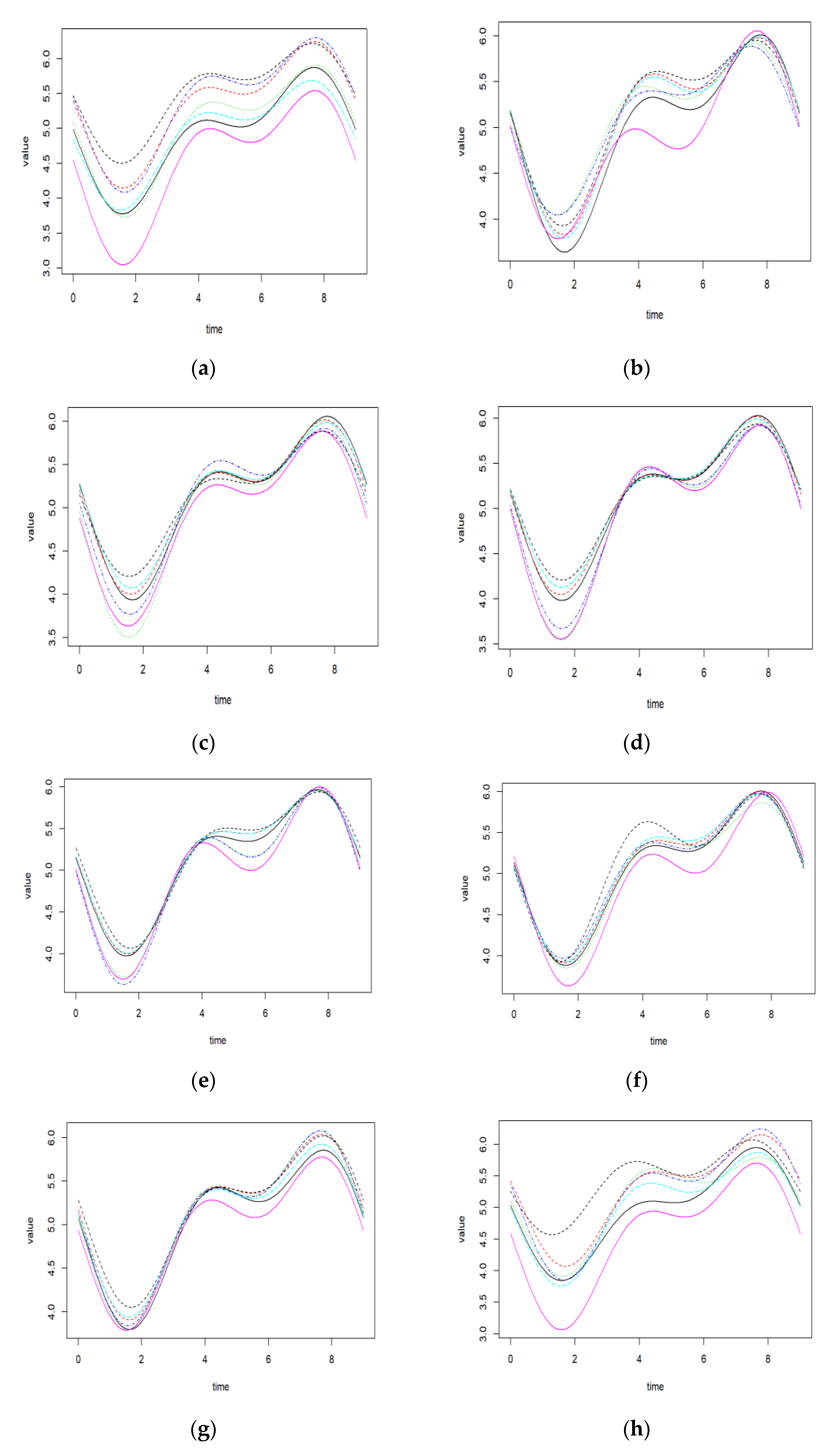
Third, we graphically plot the actual observations of onion weights and the predicted values of each environmental variable to determine the predictive power of the six environmental variables. Figure 5 shows the relationship between actual observations and predicted values.

Figure 5. Plots for actual observations and predicted values. (a) Actual values for onion weights, (b) predicted values for weights by wind speed, (c) predicted values for weights by mean temperature, (d) predicted values for weights by ground temperature, (e) predicted values for weights by humidity, (f) predicted values for weights by sunshine, (g) predicted values for weights by rain, (h) predicted values for weights by all variables.

We also calculated a Root Mean Square Error (RMSE) to numerically measure the predictive power of each environmental variable. Table 6 shows the RMSE values for six environmental variables.

Table 6. RMSE for six environmental factors and all variables.

Environmental Factors	Wind Speed	Ground Temp	Mean Temp	Humidity	Sunshine	Rain Fall	All Variables
RMSE	0.2948	0.2840	0.2940	0.3058	0.2770	0.2700	0.1300

From Figure 5 and Table 6, we can get the following results. First, all environmental variables are included in the model, and have the most predictive power. Second, among the individual environmental variables, ground temperature, sunshine, and rainfall exhibited high predictive power. Third, wind speed, mean temperature, and humidity showed the lowest predictive power.

To summarize, we discuss the following results. First, we first find that both the ground and mean temperature have a high positive correlation with the onions weights. It can also be seen that humidity has a small positive correlation with the onion weights. Finally, three of the environmental variables, such as wind speed, sunshine, and rainfall, have a small negative correlation with onion weight. Second, we can confirm that ground temperature, sunshine, and precipitation have a significant effect on onion growth and are very significant in the goodness-of-fit test. On the other hand, mean temperature, wind speed, and humidity did not significantly affect onion growth.

In conclusion, to promote onion growth, the appropriate ground temperature and amount of sunshine are essential, rainfall and humidity must be low, and appropriate wind or mean temperature must be maintained.

5. Conclusions

In the study, we applied a statistical functional regression model to investigate the relationship between various environmental factors and onion weights during the growing season. To solve this problem, we performed the following two tasks. In the first one, we identified the six most important environmental factors among those that affect onion weight during the growing season. In the second, we proposed an optimal cultivation strategy that could suggest how to manage the six identified environmental factors to maximize the onion weights.

From the analysis results so far, we could note the following facts. First, through the graphical and the correlation analysis, we can see that ground temperature, mean temperature, and humidity are positively correlated with onion weights, while wind speed, sunshine, and rainfall have a small negative correlation with the onion weights. Second, from the functional regression analysis for six environmental variables and onion weight, we note that the ground temperature, sunshine, and rainfall have a statistically significant effect on the onion weights, but other environmental factors such as wind speed, mean temperature, and humidity have little effect on the onion weights. In conclusion, to promote onion weights, the appropriate ground temperature, amount of sunshine, wind speed, and mean temperature must be maintained, and rainfall and the humidity must be low.

Future works should utilize functional data analysis to investigate how these environmental factors affect onion yields. In addition, an overall study is needed to understand how environmental and growth factors and weights and yields of onions affect each other.

References

1. Hwang, J.H. Guide to Agricultural Management: Onion Business Management; Report of Korea Rural Development Administration; Korea Rural Development Administration: Jeonju, Korea, 2015. (In Korean) [Google Scholar]
2. Kamilaries, A.; Prenafeta-Boldu, F.X. Deep learning in agriculture: A survey. Comput. Electron. Agric. 2018, 147, 70–90. [Google Scholar] [CrossRef]
3. Manikandan, K.; Vethamoni, P.I. A review: Crop modeling in vegetable crops. J. Pharmacogn. Phytochem. 2017, 6, 1006–1009. [Google Scholar]
4. Bhange, T.; Shekapure, S.; Pawar, K.; Choudhari, H. Survey Paper on Prediction of Crop yield and Suitable Crop. India Int. J. Innov. Res. Sci. Eng. Technol. 2019, 8, 5791–5795. [Google Scholar]
5. Mythra, N.; Velayudham, A.; Shamila, E.S.; Pavithra, M. A Survey on Crop Yield Prediction using Data Mining. Int. J. Comput. Trends Technol. (IJCTT) 2018, 65, 1–7. [Google Scholar]
6. Sellam, V.; Poovammal, E. Prediction of Crop Yield using Regression Analysis. Indian J. Sci. Technol. 2016, 9, 5. [Google Scholar] [CrossRef]
7. Abdelkhalik, A.; Pascual, B.; Najera, I.; Baixaulli, C.; Pascual-Seva, N. Regulated Deficit Irrigation as a Water-Saving Strategy for Onion Cultivation in Mediterranean Conditions. Agronomy 2019, 9, 521. [Google Scholar] [CrossRef]
8. Maskey, M.L.; Pathak, T.B.; Dara, S.K. Weather Based Strawberry Yield Forecasts at Field Scale Using Statistical and Machine Learning Models. Atmosphere 2019, 10, 378. [Google Scholar] [CrossRef]
9. Rathod, S.; Mishra, G.C. Statistical Models for Forecasting Mango and Banana Yield of Karnataka, India. J. Agric. Sci. Technol. 2018, 20, 803–816. [Google Scholar]
10. Villiers, M.D. Predicting Tomato Crop Yield from Weather Data Using Statistical Learning Techniques. Master’s Thesis, Commerce in Mathematical Statistics in the Faculty of Economic and Management Sciences at Stellenbosch University, Stellenbosch, South Africa, 2017. [Google Scholar]
11. Oscar, I. Start Onion Farming-The Complete Guide. 2018. Available online: https://farmingmethod.com/onion-farming-guide/ (accessed on 25 November 2019).
12. Ramsay, J.O.; Silverman, B.W. Functional Data Analysis; Springer: New York, NY, USA, 1997. [Google Scholar]
13. Ramsay, J.O.; Hooker, G.; Graves, S. Functional Data Analysis with R and MATLAB; Springer: Dordrecht, The Netherlands; Heidelberg, Germany; London, UK; New York, NY, USA, 2009. [Google Scholar]
14. Greven, S.; Scheipl, F. A general framework for functional regression modelling. Stat. Model. 2017, 17, 1–35. [Google Scholar] [CrossRef]
Article Metrics
Citations
Article Access Statistics
Multiple requests from the same IP address are counted as one view.