Graph Dilated Network with Rejection Mechanism

Abstract

Recently, graph neural networks (GNNs) have achieved great success in dealing with graph-based data. The basic idea of GNNs is iteratively aggregating the information from neighbors, which is a special form of Laplacian smoothing. However, most of GNNs fall into the over-smoothing problem, i.e., when the model goes deeper, the learned representations become indistinguishable. This reflects the inability of the current GNNs to explore the global graph structure. In this paper, we propose a novel graph neural network to address this problem. A rejection mechanism is designed to address the over-smoothing problem, and a dilated graph convolution kernel is presented to capture the high-level graph structure. A number of experimental results demonstrate that the proposed model outperforms the state-of-the-art GNNs, and can effectively overcome the over-smoothing problem.

1. Introduction

Graph structure data is ubiquitous in the real world, such as social networks [1,2,3,4,5], citation networks [6,7,8], wireless sensor networks [9], and graph-based molecules [10,11]. Recently, graph neural networks (GNNs) have aroused a surge of research interest. The goal of GNNs is to learn representation vectors of nodes in a graph, and then the learned vectors can be used in many graph-based applications, such as link prediction and node classification [12,13,14,15,16]. The general idea of GNNs is “message propagation”, i.e., each node iteratively passes, transforms, and aggregates messages (i.e., features) from its neighbors. Then, after k iterations, each node can capture the information of its neighbor nodes within k-hops.

There are many works in developing graph neural networks. GCN [17] simplifies the localized spectral filters used in [18] by weighted propagating information. GraphSAGE [6] proposes several types of aggregation strategies to propagate messages from neighbors effectively. GAT [10] adopts a self-attention [19] to dynamically propagate messages.

However, the majority of these models suffer from the “over-smoothing” problem [20,21]. Specifically, message propagation is proved to be a type of Laplacian smoothing. Stacking too many layers (i.e., repeatedly applying Laplacian smoothing many times) may lead to the representations of nodes indistinguishable and hurt the performance of GNNs [20]. Furthermore, a random walk view to message propagation shows GNNs converge to a random walk distribution [21], leading to similar conclusions with the “over-smoothing” problem.

As a matter of fact, many GNNs are shallow neural networks with only two or three layers. Thus, limited neighborhood information is captured. Moreover, adding additional layers cannot always improve the performance of GNNs, and may even have an opposite effect on GNNs [17,20]. The above discussions reflect the inability of the current GNN models in exploring the global graph structure. Therefore, although a sufficient size of neighborhoods may help models to capture the high-level graph patterns [12,20,21], most of GNNs fall into the over-smoothing problem and can only capture limited local structure of nodes.

In this paper, we focus on dealing with the limitations of current GNNs, i.e., the need and the bottleneck both introduced by the global information. In detail, we propose a rejection mechanism, which softly rejects information from distant nodes, and allows our model to be free from the over-smoothing problem. To further capture the global graph structure, a graph dilated convolution kernel is proposed, and enlarges the size of the neighborhood at each layer.

The main contributions of this paper are summarized as follows.

• We propose a novel graph neural network model, i.e., Graph Dilated networks with Rejection mechanism (GraphDRej), to learn expressive node representations.
• We design a rejection mechanism, which is a simple but effective strategy to address the over-smoothing problem.
• We present multiple graph dilated convolution kernels to explore a sufficient size of neighborhoods in message propagation.
• Extensive experimental results show that the proposed model achieves state-of-the-art results. Also, the effectiveness of both the rejection mechanism and the graph dilated convolution kernel used in GraphDRej is demonstrated.

The remainder of this paper is organized as follows. Section 2 reviews the related work. Section 3 presents the preliminaries. Section 4 analyzes the limitation of existing GNNs. Section 5 proposes GraphDRej model, i.e., Graph Dilated Network with Rejection Mechanism. Section 6 reports the experiments. Section 7 concludes the paper.

2. Related Work

Recently, a vast amount of literature has focused on analyzing graph-based problems by leveraging the graph neural networks [6,10,17,22,23,24]. GCN [17] is a pilot work, which simplifies the localized spectral filters used in [18], and extracts the 1-localized information for each node in each convolution layer. Then, the deeper relational features can be captured by stacking multiple convolution layers. GraphSAGE [6] takes the representation learning into a formal pattern, i.e., aggregation and combination, and proposes several kinds of aggregation strategies. Actually, GCN can be taken as a special case of GraphSAGE. GAT [10] considers the diversity in neighborhoods, and leverages the self-attention mechanism [19] to effectively select important information in neighborhoods. GG-NN [25] designs a gate mechanism-based aggregation function, which provides a weighted average of the messages from neighbors and the center node. Besides, there are some works [26,27] considering the imbalanced nodes in representation. Although these GNNs can characterize the node structure and learn the representations of nodes, most of them suffer from the over-smoothing problem.

Meanwhile, there are several works analyzing the mechanism of the graph neural networks, which are related to the over-smoothing problem. Li et al. (2018) [20] took graph neural networks as a special form of Laplacian smoothing, which is the main reason why GNNs work. At the same time, it shows the limitation of current GNNs, i.e., GNNs cannot capture the global graph structure due to the over-smoothing problem. Although Li et al. (2018) [20] proposed to leverage co- and self-training to improve the GNN performance, both co- and self-training are designed to deal with the limited validation issue. Therefore, the over-smoothing problem mentioned by Li et al. (2018) [20] still needs to be solved. Xu et al. (2018) [21] provide another viewpoint of GNNs. The message propagation of GNNs can be considered as a modified random walk. The distribution of influence scores between two nodes converges to a stationary distribution, which also reflects the over-smoothing problem. Xu et al. (2018) [21] proposed a densenet-like [28] module to aggregate neighbors from different hops adaptively as well as to address the over-smoothing problem. The PN [29] model proposes a novel normalization layer, which is applied on the output of the graph convolution layer to address the over-smoothing problem. Normalizing the representations of nodes can prevent these representations from being too similar. MADReg [30] provides a topological view of the over-smoothing problem and brings a MADReg loss to avoid the representations of the distant nodes to be similar to the representations of the neighbor nodes. Experimental results (see Section 6.5) show MADReg can only relieve rather than prevent this problem. Although some of these works can solve the over-smoothing problem, none of them considers how to capture a suitable larger neighborhood well to learn better node representations in a situation where GNNs are free of the over-smoothing problem. In this paper, GraphDRej can not only overcome the over-smoothing problem by a rejection mechanism, but also better characterize node structures by multiple graph dilated convolution kernels. Related experimental results are shown in Section 6.4 and Section 6.5.

3. Preliminaries

We begin with summarizing the common GNN models and, along the way, introduce our notations. We represent a graph G as $(V,E)$, where V denotes the node set and E is the edge set. Let A be the adjacency matrix of G. The k-hop neighborhood $N_k\left(v\right)$ of node v is the set of all nodes reaching to node v in k steps exactly. As default, $N\left(v\right)$ is the 1-hop neighborhood of node v. Each node $v\in V$ is associated with a feature vector $X_v$ and a label $y_v$.

Most GNNs aim to learn a node representation mapping function by using the graph structure and node features. Current GNNs follow a “message propagation” scheme, where at each iteration, the node can aggregate the information (i.e., “messages”) from its neighbors. Therefore, after k iterations of propagation, the node representation can capture k-hop structure information. Formally, at the k-th layer, a GNN can be expressed as

$$\begin{array}{c}\hfill m_v^{\left(k\right)}=\mathit{AGGREGATE}\left(\{h_u^{(k-1)}:u\in N\left(v\right)\}\right)\end{array}$$

(1)

$$\begin{array}{c}\hfill h_v^{\left(k\right)}=\mathit{COMBINE}\left(m_v^{\left(k\right)},h_v^{(k-1)}\right)\end{array}$$

(2)

where $h_v^{\left(k\right)}$ is the representation (i.e., “message”) of node v at the k-th layer, which captures the k hop structure information, and $m_v^{\left(k\right)}$ can be taken as the integrated message representation from neighbors. The initialization message $h_v^0=X_v$. AGGREGATE is a message propagation function which aggregates information from neighbors, and COMBINE is a function that combines the information from different hops. An illustration is shown in Figure 1. All the information from the neighbors (i.e., nodes 2–6) of the center node 1 is merged by AGGREGATE. Then, COMBINE combines the information from the neighbors and the center node 1.

Different models have different propagation functions. For example, Graph Convolutional Network (GCN) [17] proposes a degree-normalized algorithm to aggregate neighbors’ messages. The propagation rule (i.e., Equation (1)) of GCN can be presented as

$$\begin{array}{c}\hfill h_v^{\left(k\right)}=\sigma \left(W^{\left(k\right)}\sum _{u\in \left\{v\right\}\cup N\left(v\right)}\frac{h_u^{(k-1)}}{\sqrt{\left|N\right(u\left)\right|\left|N\right(v\left)\right|}}\right)\end{array}$$

(3)

where $W^{\left(k\right)}$ is the weight matrix. AGGREGATE and COMBINE are fused into one function (i.e., $u\in N\left(v\right)$ in Equation (1) and $u\in \left\{v\right\}\cup N\left(v\right)$ in Equation (3)), and $\sigma$ is a nonlinear function.

4. Limitation of Existing GNNs

Although GNN models significantly outperform many state-of-the-art methods on some benchmarks, there remain some problems that limit the performance of GNNs.

In point of fact, the message propagation scheme in GNNs can be taken as a random walk [21]. The influence score of node u on node v, which measures the effect of the input feature of node u to the representation of node v, can be defined as

$$\begin{array}{c}\hfill I(v,u)=\sum _i\sum _j\left|\frac{\partial h_{v,i}^{\left(k\right)}}{\partial h_{u,j}^{\left(0\right)}}\right|\end{array}$$

(4)

where $h_v^{\left(k\right)}$ is the representation vector of node v at the k-th layer, $h_{v,i}^{\left(k\right)}$ refers to the i-th dimension of $h_v^{\left(k\right)}$, and $h_u^{\left(0\right)}=X_u$. Then, the expected distribution of the normalized influence score follows a slightly modified k-step random walk distribution $P\left(u\right|v,k)$ starting at the root node v [21]. Thus, the message propagates from node u to node v in a random walk pattern.

As we know, the node sequence $(v_t:t=0,1,\dots )$ generated by a random walk is a Markov chain. When $k\to \infty$, the probability distribution $P\left(u\right|v,k\to \infty )$ converges to a stationary distribution (i.e., $P\left(o\right|x)\equiv P(o\left|y\right)$ for any node $x,y,o\in V$) [31]. It means that, for the message propagation scheme, the representation of each node is influenced almost equally by any other nodes (i.e., $I(x,o)\approx I(y,o)$) [21] when GNNs go deeper (i.e., a large value of k). In other words, the node representations may be over-smoothed and lose their focus by the information from distant nodes [20], which is called the over-smoothing problem.

Therefore, one of the limitations of existing GNNs is that most GNN models cannot go deeper. A deeper version of these models even performs worse than a shallow version, and the best performance of these models is usually achieved within two or three layers [17]. Although a sufficient size of neighborhoods is especially important, which allows the models to explore a more complex graph structure and aggregate useful neighbors’ information [20,21], existing GNNs can only capture limited structure information in a small size of the neighborhoods.

In summary, on the one hand, when we stack too many layers in a GNN model, the node representation will be over smoothed, which makes the node representation indistinguishable. On the other hand, there always exists a need for a sufficient size of neighborhoods to learn a more effective representation [20,21]. Therefore, in this paper, we propose a new neural network architecture to tackle the over-smoothing problem and capture a larger size of neighborhoods at the same time.

5. Graph Dilated Network with Rejection Mechanism

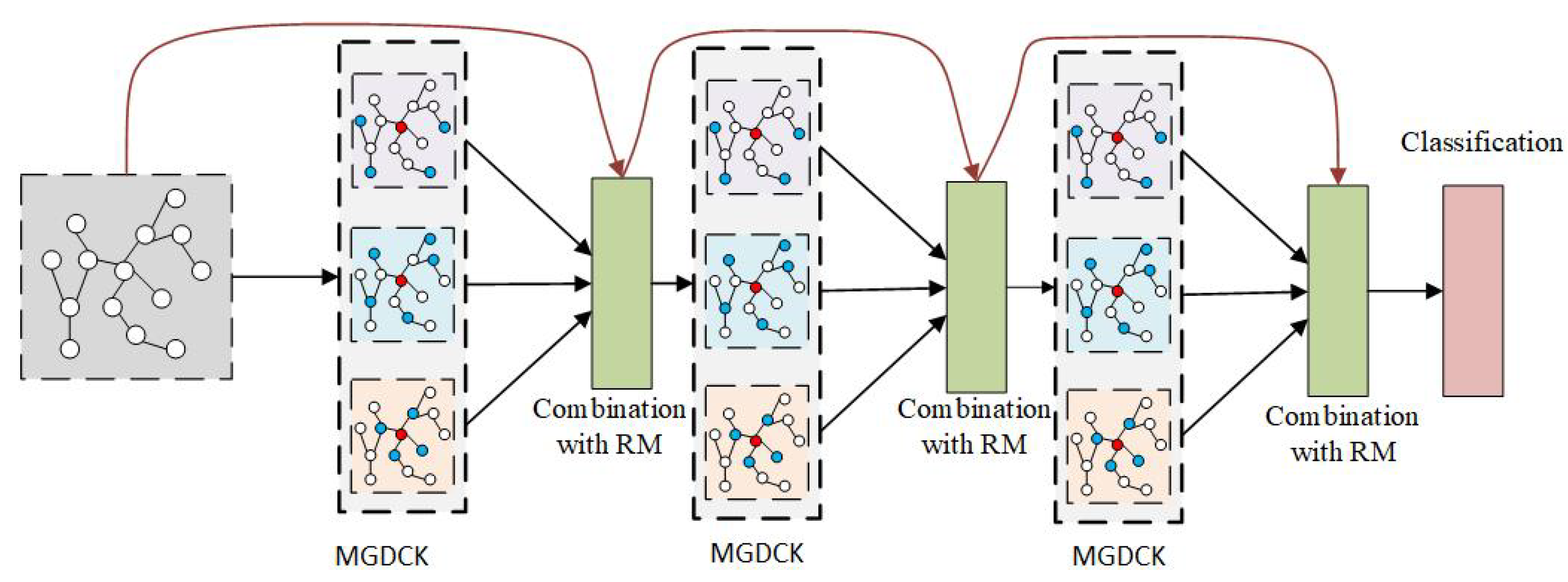
In this section, we introduce the proposed model, called Graph Dilated network with Rejection mechanism (GraphDRej). To overcome the conflict of GNNs just shown in the preceding section, we propose two main components, i.e., the rejection mechanism and the graph dilated convolution kernel. Generally speaking, at each layer, each node can aggregate messages from a large neighborhood via graph dilated convolution kernels, and a hop penalty parameter is introduced to implicitly reject the information from distant nodes (addressing the over-smoothing problem). At the last layer, a cross-entropy loss is adopted to optimize the parameters of the proposed model. Figure 2 illustrates the architecture of the proposed model.

5.1. Rejection Mechanism

5.1.1. Method

To address the over-smoothing problem, we propose a simple but effective Rejection Mechanism (RM). As discussed in Section 4, the over-smoothing problem is caused by averaging too much information from distant neighbors. Therefore, we introduce a learnable hop penalty parameter $c^{\left(k\right)}\in R$ (optimized by the backpropagation) at each layer to adaptively control the messages flowing from one layer to the next layer (i.e., from one hop to the next hop). In this way, the model can reject the messages from distant nodes to address the over-smoothing problem.

Different from GAT, which dynamically selects messages from 1-hop neighbors, the rejection mechanism is a layer-wise or hop-wise operation. Specifically, the rejection mechanism focuses on the combination function (i.e., Equation (2)) introduced in the message propagation. At the k-th layer, the hop penalty parameter $c^{\left(k\right)}$ is applied into the integrated message representation from neighbors, and then the combination function can be rewritten as

$$\begin{array}{cc}\hfill & c^{{\left(k\right)}^{\prime }}=\mathit{sigmoid}\left(c^{\left(k\right)}\right)\hfill \\ \hfill & h_v^{\left(k\right)}=\sigma \left(W^{\left(k\right)}\left(h_v^{(k-1)}\oplus c^{{\left(k\right)}^{\prime }}\odot m_v^{\left(k\right)}\right)\right)\hfill \end{array}$$

(5)

where $W^{\left(k\right)}$ is a weight matrix, $c^{{\left(k\right)}^{\prime }}\in [0,1]$ is the rescaled penalty parameter, and ⊙ refers that each element of the vector $m^{\left(k\right)}$ multiplies the rescaled hop penalty parameter $c^{{\left(k\right)}^{\prime }}$. Intuitively, the value of $c^{{\left(k\right)}^{\prime }}$ can be regarded as a gate to influence the message propagation from neighbors to the center node. $\oplus$ is an element-wise addition operation.

To fully understand the proposed rejection mechanism, we provide an example (shown in Figure 3) to illustrate how it works to address the over-smoothing problem. For simplicity, a chain graph containing four nodes is taken as an example, and only considers the predecessor nodes as 1-hop neighbors. Considering a three-layer graph neural network, which adopts the mean aggregation function and the proposed combination function with RM, the propagation in the k-th layer for this chain graph can be expressed as (ignoring the weight matrix and nonlinear function in Equation (5))

$$\begin{array}{cc}\hfill m_i^{\left(k\right)}& =h_{i-1}^{(k-1)}\hfill \end{array}$$

(6)

$$\begin{array}{cc}\hfill h_i^{\left(k\right)}& =h_i^{(k-1)}\oplus c^{\left(k\right)}{m}_i^{\left(k\right)}\hfill \\ \hfill & =h_i^{(k-1)}\oplus c^{\left(k\right)}{h}_{i-1}^{(k-1)}\hfill \end{array}$$

(7)

where $i,k\in \{1,2,3\}$, the symbol ⊙ in Equation (5) is ignored for expressing convenience, and $c^{\left(k\right)}$ refers to the rescaled parameter $c^{{\left(k\right)}^{\prime }}$.

Then, the node 3’s representation obtained from the last layer, can be represented as

$$\begin{array}{cc}\hfill h_3^{\left(3\right)}=& h_3^{\left(0\right)}\oplus (c^{\left(1\right)}+c^{\left(2\right)}+c^{\left(3\right)})h_2^{\left(0\right)}\hfill \\ \hfill & \oplus (c^{\left(1\right)}{c}^{\left(2\right)}+c^{\left(1\right)}{c}^{\left(3\right)}+c^{\left(2\right)}{c}^{\left(3\right)})h_1^{\left(0\right)}\hfill \\ \hfill & \oplus c^{\left(1\right)}{c}^{\left(2\right)}{c}^{\left(3\right)}{h}_0^{\left(0\right)}.\hfill \end{array}$$

(8)

It reveals that the influence from the distant node 0 to the representation of node 3 is punished by ${\prod }_{k=1}^3{c}^{\left(k\right)}$. Due to $c^{\left(k\right)}\in [0,1]$, multiple multiplications will lead to a small value, which adaptively controls the message flowing from distant nodes (e.g., node 0) to the representation node (e.g., node 3).

Therefore, the benefits of the proposed rejection mechanism can be summarized as follows. (1) When stacking layers to build a deep GNN, the information from distant nodes will be more likely to be punished or even rejected. It is a simple but effective way to address the over-smoothing problem. (2) The information from distant nodes can also affect the node representation, which helps to capture the global structure. (3) The combination of the hop penalty parameters leads to adaptively aggregate information from different hops, which contributes to building a more powerful deep graph model.

5.1.2. Discussion

We notice that the graph neural network GG-NN [25] proposes a gate mechanism to aggregate neighbors, which is similar to the rejection mechanism proposed in our paper. The differences between these two mechanisms are summarized as follows. (1) The motivations of these two mechanisms are different. For GG-NN, the gate mechanism is proposed to dynamically aggregate neighbors’ information based on the information of neighbors and the center node. For GraphDRej, the rejection mechanism is proposed to reject the information from distant nodes to address the over-smoothing problem. (2) The rejection mechanism is simpler and does not require much computation, whereas for GG-NN, the gate computation involves several multiplication and addition operations of matrices [25]. (3) The rejection mechanism is a more direct way that strictly limits the information from the distant nodes by the penalty parameters, whereas in GG-NN, according to Equation (6) in the original paper of GG-NN [25], not only the messages from the neighbors are rescaled, but also the message from the center node is rescaled. This means the gate mechanism in GG-NN is more like a weighted average of the message from neighbors and the center node, and the messages from the center node may also be rejected. Experimental results (see Section 6.6) show GG-NN still suffers from the over-smoothing problem.

To further analyze the connection between the rejection mechanism and the gate mechanism, we propose a gate-based version of GraphDRej (denoted as GraphDRej-Gate). The only difference between GraphDRej and GraphDRej-Gate is the computation of the penalty parameter. The penalty parameter $c^{\left(k\right)}$ in GraphDRej is used for all the nodes in the same layer, whereas the penalty parameter $c_v^{\left(k\right)}$ in GraphDRej-Gate is used for node v in the same layer.

$$\begin{array}{c}\hfill c_v^{\left(k\right)}=\mathit{sigmoid}\left(W^{\left(k\right)}{m}_v^{\left(k\right)}+U^{\left(k\right)}{h}_v^{(k-1)}\right)\end{array}$$

(9)

where $W^{\left(k\right)}$ and $U^{\left(k\right)}$ are the transformation matrices. Compared with GG-NN, the rejection (gate) mechanism in GraphDRej-Gate is only applied to the neighbors’ messages, which helps to address the over-smoothing problem (see Section 6.6). Note that although the gate mechanism is common in other research areas, how to apply the gate mechanism on GNNs to address the over-smoothing problem is still an open question. For example, GG-NN falls into the over-smoothing problem, while GraphDRej-Gate can solve this problem. Actually, the rejection mechanism is a more general idea and leads to a direction on addressing this problem, and the penalty parameter can be a simple learnable parameter or can be computed by a gate function.

5.2. Graph Dilated Convolution Kernel

To have a sufficient size of neighborhoods in message propagation, we explore the idea of dilated convolution kernel [32] used in Computer Version to enlarge the reception field. Then, we propose a graph dilated convolution kernel, which changes the standard and single message propagation scheme, i.e., one layer for searching 1-hop neighbors, and brings the diversity of propagation schemes.

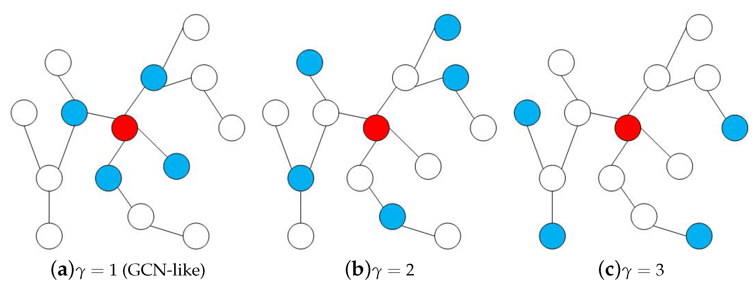
Specifically, we introduce a graph dilation rate $\gamma$, which refers to the distance between the node and its neighbor nodes. Figure 4 illustrates the examples of graph dilated convolution kernels with $\gamma \in \{1,2,3\}$. Actually, the standard graph convolution kernels used in GNNs can be taken as a special case of our graph dilated convolution kernel where $\gamma =1$. Obviously, a larger value of $\gamma$ allows the model to explore nodes from a larger neighborhood. For example, a two-layer stacked graph dilated convolution ($\gamma =3$) network can view neighbors within six hops, whereas for a standard two-layer stacked graph convolution network, only neighbors in two hops are considered. Therefore, we can enlarge the neighborhood size via graph dilated convolution kernels.

As presented above, different graph dilated convolution kernels take nodes in different hops as the neighborhoods. To have a diverse and sufficient size of neighborhoods, multiple types of graph dilated convolution kernels are simultaneously applied to the center node. Then, we further propose Multi Graph Dilated Convolution Kernels (MGDCK). At each k-th layer, multiple types of graph dilated convolution kernels are adopted. Each node v may aggregate the messages not only from 1-hop neighbors (i.e., $N\left(v\right)$), but also from 2-hop neighbors (i.e., $N_2\left(v\right)$). Formally, when each layer contains T types of graph dilated convolution kernels, the AGGREGATE and COMBINE functions can be expressed as

$$\begin{array}{cc}\hfill & m_v^{(k,t)}=\mathit{AGGREGATE}\left(\left\{h_u^{(k-1,t)}:u\in N_t\left(v\right)\right\}\right)\hfill \end{array}$$

(10)

$$\begin{array}{cc}\hfill & h_v^{(k,t)}=\mathit{COMBINE}\left(m_v^{(k,t)},h_v^{(k-1,t)}\right)\hfill \end{array}$$

(11)

where $t\in \{1,2,3,\dots ,T\}$, COMBINE refers to the combination function with RM mentioned in Section 5.1, and the implementation of AGGREGATE can be various. In this paper, we adopt a mean aggregation strategy. Other aggregation functions can also be applied. Then, the representation of node v at the k-th layer is the mean of all the representation vectors produced by T graph dilated convolution kernels

$$\begin{array}{c}\hfill h_v^{\left(k\right)}=\mathit{mean}\left(\left\{h_v^{(k,t)}:t\in \{1,2,3,\dots ,T\}\right\}\right).\end{array}$$

(12)

Note that other pooling strategies such as max-pool, min-pool, and attention-pool can also be considered as the summarization operators on all the representations from these T graph dilated convolution kernels. Here, we only take the mean-pool as an example.

Although directly stacking layers can also enlarge the size of neighborhoods, too many layers may introduce the difficulty of the model training. The experimental results also show the effectiveness of graph dilated kernels compared with the directly stacking strategy (see Section 6.7).

5.3. Training

In this section, we introduce the training details of GraphDRej, including the loss function and the overall algorithm.

5.3.1. Loss Function

We follow the loss used in standard GNNs [6,10,17]. The loss function of GraphDRej is a supervised loss, i.e., making a prediction for the label of each training node. The supervised loss is defined as the cross-entropy.

$$\begin{array}{cc}\hfill z_v& =\mathit{softmax}\left(W_z{h}_v^{\left(K\right)}\right)\hfill \end{array}$$

(13)

$$\begin{array}{cc}\hfill \mathit{Loss}& =\sum _v{y}_v\mathit{ln}{z}_v\hfill \end{array}$$

(14)

where $W_z$ is a weight matrix, $h_v^{\left(K\right)}$ is the output of last layer and is taken as the learned node representation vector, and $z_v$ is the label prediction of node v in the training nodes.

5.3.2. Overall Algorithm

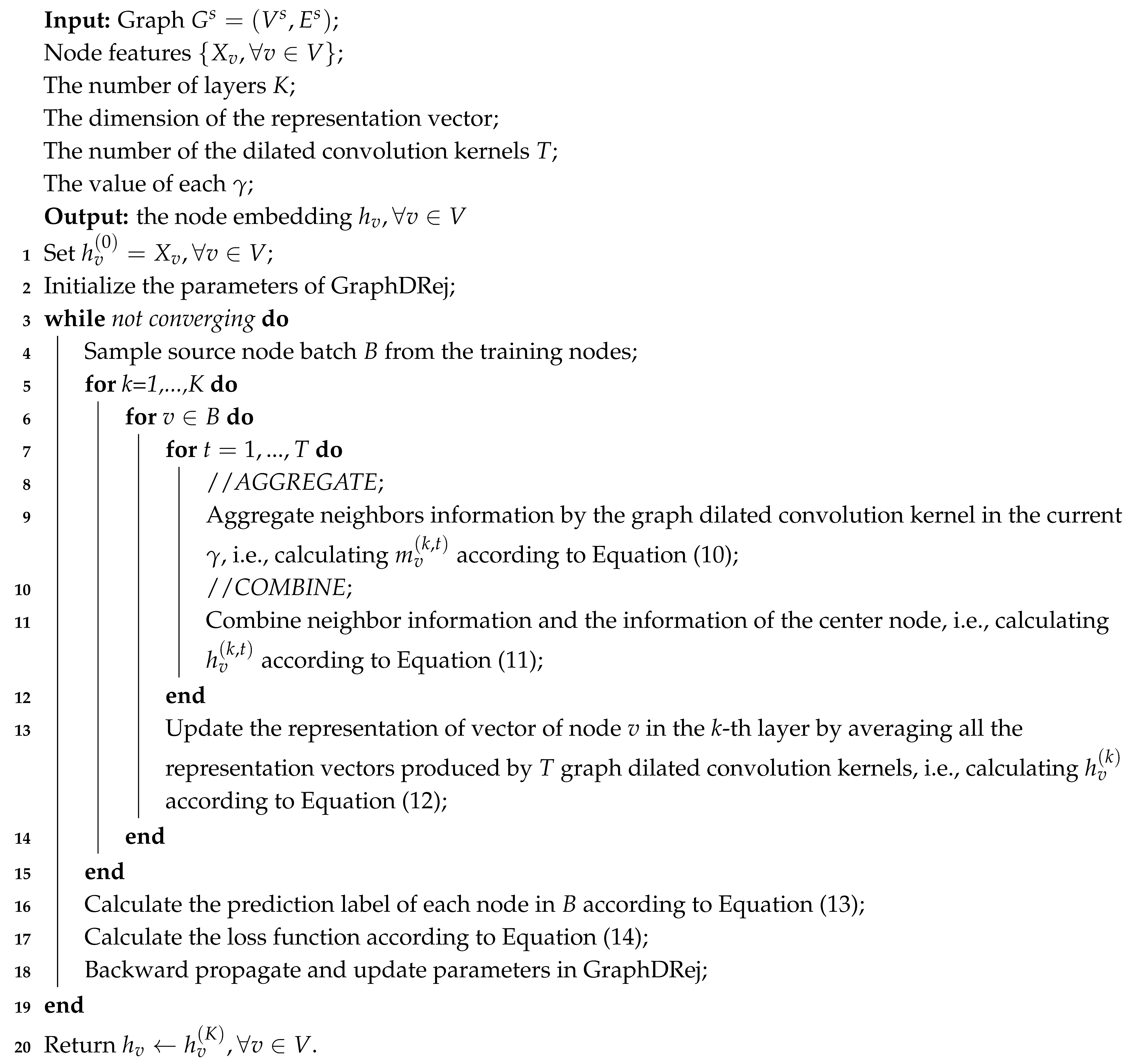
The overall algorithm of GraphDRej is summarized in Algorithm 1. First, in each iteration, we sample a batch of nodes from the training nodes in Line 4. At each layer k, multiple graph dilated convolution kernels are applied to aggregate information from neighbors (Lines 8–9), and a rejection mechanism based combination is adopted to combine the information from the neighbors and the center node (Lines 10–11). Then, the node representation vector is updated by averaging the representation produced by different graph dilated convolution kernels (Line 13). We calculate the label prediction and the cross-entropy loss in Lines 16–17. After the forward propagation (Lines 4–17), backward propagation is carried out to update the parameters in Line 18. Finally, after the convergence, we take the last layer output as the embeddings of nodes in Line 20.

Algorithm 1: The Algorithm of GraphDRej.

6. Experiments

We evaluate the benefits of GraphDRej against a number of state-of-the-art graph neural networks with the goal of answering the following questions.

Q1. 

How does the GraphDRej perform in comparison to the state-of-the-art GNNs?

Q2. 

Can the proposed rejection mechanism address the over-smoothing problem?

Q3. 

How much improvement is provided by multiple graph dilated convolution kernels?

6.1. Data Sets

To adequately evaluate the performance of our model and baselines, the experiments are conducted on three real-world data sets.

Cora 

is a research paper-based graph. It contains 2708 machine learning papers from seven classes and 5429 links between them. The links are citation relationships among the papers. Each paper is described by a binary vector of 1433 dimensions, indicating the presence of the corresponding words.

Citeseer 

is another research based graph that contains 3327 publications from six classes and 4732 links between them. Similar to Cora, the links are citation relationships among these papers, and each paper is described by a binary vector of 3703 dimensions.

Pubmed 

is also a citation graph, and contains 19,717 papers from three classes as well as 44,338 links between them. Similar to Cora, the links are citation relationships among the papers, and each paper is described by a binary vector of 500 dimensions.

The statistics of the data sets are presented in

Table 1. Data set information.

Data Set	#Nodes	#Edges	#Class	#Features
Cora	2708	5429	7	1433
Citeseer	3327	4732	6	3703
Pubmed	19,717	44,338	3	500

.

6.2. Baselines

In the performance comparison, we consider the state-of-the-art baselines based on GNNs.

GCN 

[17] is a graph convolution neural network, which simplifies the localized spectral filters used in [18], and extracts the 1-localized information for each node in each convolution layer.

GraphSAGE 

[6] extends GCN to a more general way, and introduces two basic functions, i.e., the aggregation function and the combination function.

GAT 

[10] employs the idea of self attention [19] to filter important messages from neighbors.

JK 

[21] deals with the over-smoothing problem, which uses a densenet-like [28] module to adaptively aggregate neighbors information from different hops.

PN 

[29] proposes a novel normalization layer which is applied on the output of the graph convolutional layer. In this way, PN can address the over-smoothing problem.

MADReg 

[30] also focuses on the over-smoothing problem. It takes the gap of MAD values (MADGap) as a regularization term to avoid the representations of distant nodes to be similar.

GG-NN 

[25] proposes a gate mechanism to aggregate the messages from neighbors.

GraphDRej-Gate 

is a gate version of GraphDRej, in which the penalty parameter is calculated by a gate function.

6.3. Experimental Setting

We set the dimension of the representation vector to 16 for all models. Moreover, we use the pooling aggregation in GraphSAGE, which achieves the best performance compared to other aggregation strategies, (as discussed in [6]). For JK, we use the Maxpool for the same reason as GraphSAGE. All models are trained using the Adam SGD optimizer [33] with an initial learning rate of 0.01. We use dropout rate $d=0.2$ for all layers. For all data sets, we take 20% nodes as the training nodes, 40% nodes as the validation nodes, and the rest 40% as the test nodes. We use an early stopping strategy on both the model loss and accuracy score on the validation nodes, with the patience of 20 epochs.

6.4. Results for Node Classification Task

To fully evaluate the performance of GraphDRej (including RM and MGDCK) and baselines, we not only report the classification accuracy (shown in

Table 2. Node classification accuracy (%) for two-layer graph neural networks (GNNs). The list in parentheses next to the accuracy of GraphDRej refers to the value set of $\gamma$ adopted by the corresponding GraphDRej on different data sets.

Method\Data Sets	Cora	Citeseer	Pumbed
GraphSAGE	76.20	71.00	84.54
GCN	79.98	71.90	80.70
GAT	76.66	70.85	84.62
JK	74.82	71.53	84.75
PN	75.46	71.83	83.64
MADReg	76.38	71.07	84.56
GG-NN	73.99	70.85	84.62
GraphDRej	81.00 ($\mathit{\gamma }=[\mathbf{1},\mathbf{2}]$)	72.58 ($\mathit{\gamma }=[\mathbf{1},\mathbf{2}]$)	85.39 ($\mathit{\gamma }=[\mathbf{1},\mathbf{2}]$)

) of these models with the same two layers but also report the best results (presented in

Table 3. The best performance for GNNs on the node classification task. For baselines, the number in parentheses next to the accuracy indicates the best performing number of layers. For GraphDRej, the first number in parentheses has the same meaning as that in baselines, and the second list in parentheses refers to the value set of $\gamma$ adopted by the corresponding GraphDRej.

Method\Data Sets	Cora	Citeseer	Pumbed
GraphSAGE	80.54 (6)	71.45 (4)	84.54 (2)
GCN	80.26 (4)	71.90 (2)	80.70 (2)
GAT	80.54 (6)	70.85 (2)	84.62 (2)
JK	81.83 (9)	71.53 (2)	85.32 (4)
PN	79.34 (6)	71.83 (2)	83.67 (2)
MADReg	81.37 (6)	71.30 (4)	84.56 (2)
GG-NN	77.40 (4)	70.85 (2)	84.85 (4)
GraphDRej	83.39 (3, [1,2])	72.58 (2, [1,2])	85.47 (2, [1,2,3])

) achieved by these models with different numbers of layers. These results provide the positive evidence to question Q1: GraphDRej significantly outperforms previous models both on the two-layer results and on the best results over all data sets. For the tasks with the two-layer models, GraphDRej achieves an improvement ranging from 0.68% to 6.18% over all data sets. Also, compared with the best results, GraphDRej achieves gains from 0.15% to 4.77% over all data sets. Furthermore, compared with the GNNs (i.e., JK, PN, and MADReg), which consider the over-smoothing problem, GraphDRej also achieves the best performances. Although GG-NN adopts a gate mechanism which is similar to our proposed rejection mechanism, GraphDRej can also outperform GG-NN (further analysis can be found in Section 6.6). These analyses show the effectiveness of GraphDRej on learning a more meaningful node representation.

6.5. Evaluation of Rejection Mechanism

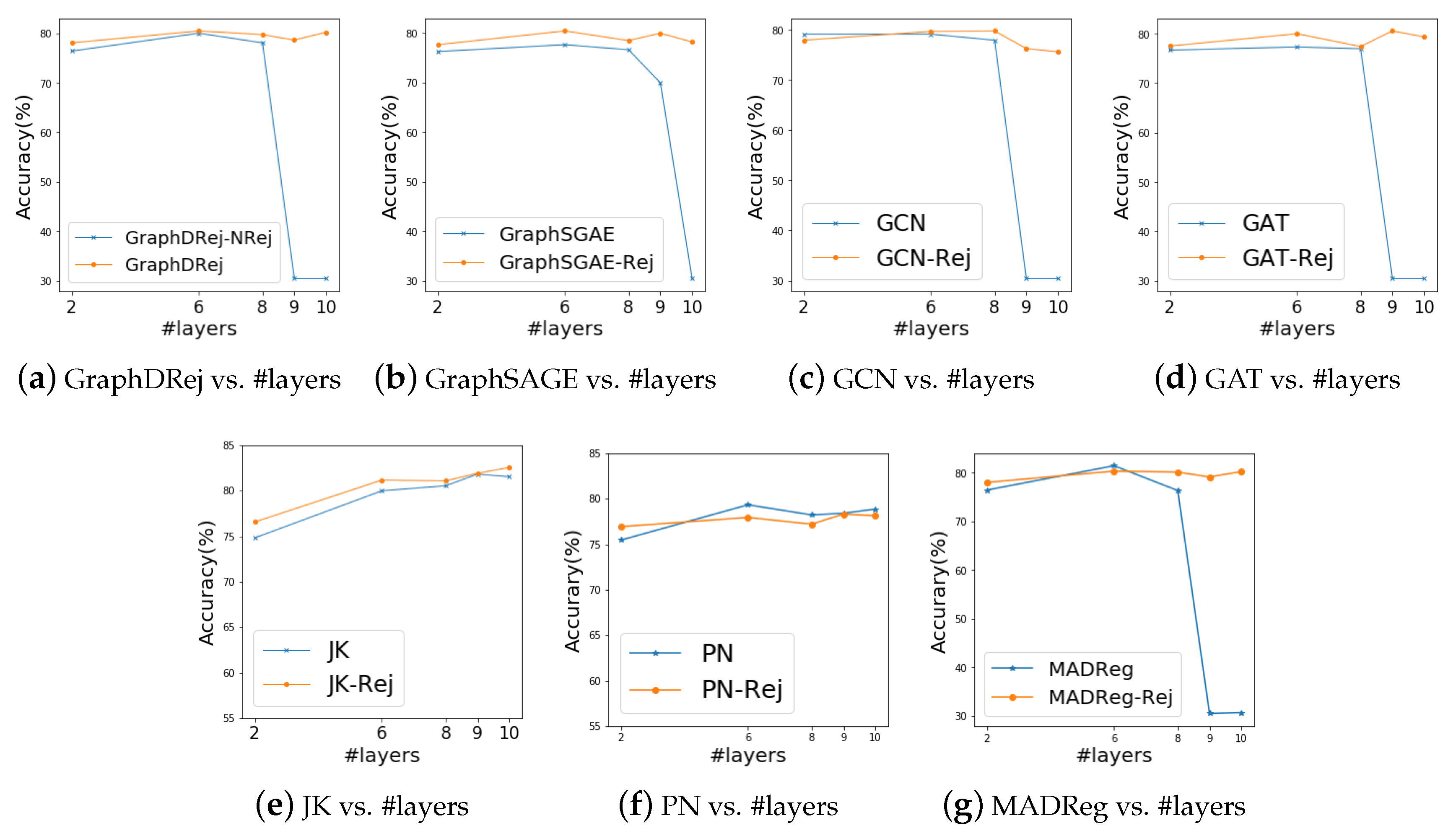
Actually, the proposed rejection mechanism (RM) is a general method to address the over-smoothing problem. Therefore, we apply the RM to other GNN models to evaluate whether RM can help these GNNs to prevent the over-smoothing problem (i.e., answering the question Q2). Additionally, we also provide the results of GraphDRej to show the effectiveness of RM. Furthermore, to avoid the influence of multiple dilated convolution kernels, for GraphDRej, we apply a single dilated convolution kernel with $\gamma =1$ (i.e., a GCN-like kernel). The results on Cora in terms of classification accuracy are presented in Figure 5 (similar performance trends are also observed on other data sets).

Some observations can be summarized as follows.

Evaluation with the standard GNNs. First, we evaluate the RM with the standard GNNs, which suffer the over-smoothing problem. As shown in Figure 5a–d, when we gradually increase the number of layers, most of the original models fail in the over-smoothing problem. Specifically, when it comes to a deeper model (e.g., the layer of GNNs is 9 or 10 in Figure 5), the performance of most of these models sharply decreases, which also supports the discussion mentioned in Section 4. When we apply RM to these failed models, all of these models in a deep version obviously overcome the over-smoothing problem and achieve high performances. Thus, it indicates the rejection mechanism is indeed beneficial to solving the over-smoothing problem.

Evaluation with the GNNs, which also address the over-smoothing problem. Then, we evaluate the RM with the GNNs (i.e., JK [21], PN [29], and MADReg [30]), which also address the over-smoothing problem. (1) As seen in Figure 5e–f, both JK and PN can well solve the over-smoothing problem, as the performances do not drop sharply with the increasing of the layer number. (2) As shown in Figure 5g, it seems that the over-smoothing problem still exists in MADReg. Similar conclusions can be found in the original paper of MADReg [30]. Specifically, from Table 5 in [30], we can find that although MADReg can improve the performance of the standard GNNs, the performance of a GNN with the MADReg in a deep version is far away from the performance of that in a shallow version. (3) Then, we apply RM on these GNNs (including JK, PN, and MADReg). JK still can be improved by RM. PN-Rej achieves comparable performance with PN. For MADReg, as discussed above, MADReg cannot well address the over-smoothing problem. With the help of RM, MADReg-Rej can achieve a big improvement and address the over-smoothing problem.

6.6. Evaluation between Rejection Mechanism and Gate Mechanism

To further analyze the rejection mechanism, we conduct experiments to evaluate the performances between the rejection mechanism and the gate mechanism. In order to avoid the influence of multiple graph dilated convolution kernels, the variants of GraphDRej (including GraphDRej and GraphDRej-Gate) used in this section only adopt a single kernel, i.e., $\gamma =1$. The nodes classification results with the different number of layers are reported in

Table 4. Rejection mechanism vs. gate mechanism. We report the accuracy (%) of nodes classification with different numbers of layers on Cora.

Method\#layers	1	2	3	4	5	6	7	8	9	10
GG-NN	67.90	73.99	76.66	77.40	76.01	30.44	30.44	30.44	30.44	30.44
GraphDRej	73.52	78.04	79.43	79.61	80.17	80.44	80.26	79.70	78.60	80.17
GraphDRej-Gate	71.31	76.94	79.70	80.17	80.81	80.44	80.90	79.43	80.54	73.80

. It shows that the performance of GG-NN drops quickly when the number of layers increases. It indicates that although GG-NN adopts a gate mechanism, the over-smoothing problem still exists, whereas for GraphDRej-Gate, it successfully overcomes this problem and achieves comparable performance with GraphDRej. It shows the main factor to solve the over-smoothing problem is to reject the message from distant nodes with the penalty parameter, which can be implemented by a learnable parameter or a gate function.

6.7. Evaluation of Multiple Graph Dilated Convolution Kernels

To address Q3, we design two types of classification tasks. In order to avoid the influence of RM, the variants of GraphDRej used in this subsection disable RM temporarily.

6.7.1. Evaluation of GraphDRej with the Same Number of Layers

We provide three variants of GraphDRej: GraphDRej-1, GraphDRej-2, and GraphDRej-3. All of these three models have two layers. The only difference among them is that GraphDRej-1 adopts a single graph dilated convolution kernel with $\gamma =1$ at each layer, GraphDRej-2 adopts two types of graph dilated convolution kernels with $\gamma \in \{1,2\}$ at each layer, and GraphDRej-3 contains three types of graph dilated convolution kernels with $\gamma \in \{1,2,3\}$. This means that although all of these models have the same number of layers, the total size of neighborhoods is different. The statistics of these versions are summarized in

Table 5. The statistics for graphDRej variants.

Variants	#Layers	$\mathit{\gamma }$	#Neighborhood
GraphDRej-1	2	[1]	2
GraphDRej-2	2	[1,2]	4
GraphDRej-3	2	[1,2,3]	6
GraphDRej-1-6	6	[1]	6
GraphDRej-2-3	3	[1,2]	6
GraphDRej-3-2	2	[1,2,3]	6

. The results are reported in

Table 6. The accuracy (%) for evaluation of GraphDRej with the same number of layers on Cora.

Variants	GraphDRej-1	GraphDRej-2	GraphDRej-3
Accuracy	76.38	79.61	79.70

. We observe that enlarging the neighborhood size in a GNN layer can improve the model performance, and achieve gains 3.32% and 3.23%, respectively (compared to GraphDRej-1). Furthermore, compared to the results of GraphDRej-2 and GraphDRej-3, too large a size of neighborhoods may not further improve the performance. The reasons for this are as follows. (1) On the one hand, adopting a larger size of neighborhoods is easier for models to overfitting the training data, which may influence the generalization of the model and lead to a worse performance. (2) On the other hand, not all the nodes are useful to characterize the representation of the center node, and the distant nodes are likely to bring noise [30]. Therefore, a larger size of neighborhoods is more likely to introduce some noise nodes (e.g., distant node) in representation. Therefore, it indicates that a suitable size of neighborhoods is needed, which can enable GraphDRej to explore sufficient neighbors’ structure and avoid overfitting as well as the negative effect of noise nodes.

6.7.2. Evaluation of GraphDRej with the Same Size of Neighborhoods

We also design another three variants of GraphDRej, denoted as GraphDRej-1-6, GraphDRej-2-3, and GraphDRej-3-2. The details of these versions can be found in Table 5. Generally speaking, although these three variants contain different numbers of layers and different kinds of graph convolution dilated kernels, all of these models capture the same size of neighborhoods, i.e., 6-hop-based neighborhoods. The results are reported in

Table 7. The accuracy (%) for evaluation of GraphDRej with the same size of neighborhoods on Cora.

Variants	GraphDRej-1-6	GraphDRej-2-3	GraphDRej-3-2
Accuracy	79.98	82.10	79.70

. Although these models capture the same size of neighborhoods, GraphDRej-2-3 outperforms the other two variants significantly, and can better characterize the structure information. It demonstrates the effectiveness of graph dilated convolution kernels, and also shows a well-designed graph dilated convolution architecture is needed.

7. Conclusions

In this paper, we first analyze the limitations of existing GNNs, i.e., the need and the bottleneck both introduced by the global information. Then a rejection mechanism is designed, which is a concise but effective way to address the over-smoothing problem. Next, we propose a graph dilated convolution kernel, which enlarges the size of the neighborhood at each layer. Extensive experimental results demonstrate that the proposed model achieves state-of-the-art results. In the future, we will pay more attention to the analysis of how to design a good architecture for graph dilated networks with RM to capture graph information as much as possible.

References

1. Tang, W.; Luo, G.; Wu, Y.; Tian, L.; Zheng, X.; Cai, Z. A Second-Order Diffusion Model for Influence Maximization in Social Networks. IEEE Trans. Comput. Soc. Syst. 2019, 6, 702–714. [Google Scholar] [CrossRef]
2. Lee, R.C.; Cuzzocrea, A.; Lee, W.; Leung, C.K. An innovative majority voting mechanism in interactive social network clustering. In Proceedings of the 7th International Conference on Web Intelligence, Mining and Semantics, Amantea, Italy, 19–22 June 2017; p. 14. [Google Scholar]
3. Zhang, M.; He, Z.; Hu, H.; Wang, W. E-rank: A structural-based similarity measure in social networks. In Proceedings of the 2012 IEEE/WIC/ACM International Conferences on Web Intelligence and Intelligent Agent Technology, Macau, China, 4–7 December 2012; Volume 1, pp. 415–422. [Google Scholar]
4. Wang, M.; Wang, C.; Yu, J.X.; Zhang, J. Community Detection in Social Networks: An In-depth Benchmarking Study with a Procedure-Oriented Framework. Proc. VLDB Endow. 2015, 8, 998–1009. [Google Scholar] [CrossRef] [Green Version]
5. Huang, B.; Wang, C.; Wang, B. NMLPA: Uncovering Overlapping Communities in Attributed Networks via a Multi-Label Propagation Approach. Sensors 2019, 19, 260. [Google Scholar] [CrossRef] [PubMed] [Green Version]
6. Hamilton, W.; Ying, Z.; Leskovec, J. Inductive representation learning on large graphs. In Advances in Neural Information Processing Systems; MIT Press: Long Beach, CA, USA, 2017; pp. 1024–1034. [Google Scholar]
7. Hamilton, W.L.; Ying, R.; Leskovec, J. Representation learning on graphs: Methods and applications. arXiv 2017, arXiv:1709.05584. [Google Scholar]
8. Yan, B.; Wang, C. NEOKNN: A Network Embedding Method Only Knowing Neighbor Nodes. In Proceedings of the 26th International Conference Neural Information Processing ICONIP 2019, Sydney, NSW, Australia, 12–15 December 2019; pp. 523–531. [Google Scholar]
9. Yang, Y.; Gao, H.; Li, J.; Shi, S. A Distributed and Kernel-Based Scheme for Location Verification in Wireless Sensor Networks. Ad Hoc Sens. Wirel. Netw. 2013, 18, 333–351. [Google Scholar]
10. Veličković, P.; Cucurull, G.; Casanova, A.; Romero, A.; Liò, P.; Bengio, Y. Graph Attention Networks. In Proceedings of the International Conference on Learning Representations, Vancouver, BC, Canada, 30 April–3 May 2018. [Google Scholar]
11. Zhang, D.; Yin, J.; Zhu, X.; Zhang, C. Network Representation Learning: A Survey. IEEE Trans. Big Data 2020, 6, 3–28. [Google Scholar] [CrossRef] [Green Version]
12. Grover, A.; Leskovec, J. node2vec: Scalable feature learning for networks. In Proceedings of the 22nd ACM SIGKDD International Conference on Knowledge Discovery and Data Mining, San Francisco, CA, USA, 13–17 August 2016; pp. 855–864. [Google Scholar]
13. Perozzi, B.; Al-Rfou, R.; Skiena, S. Deepwalk: Online learning of social representations. In Proceedings of the 20th ACM SIGKDD International Conference on Knowledge Discovery and Data Mining, New York, NY, USA, 24–27 August 2014; pp. 701–710. [Google Scholar]
14. Goyal, P.; Ferrara, E. Graph embedding techniques, applications, and performance: A survey. Knowl. Based Syst. 2018, 151, 78–94. [Google Scholar] [CrossRef] [Green Version]
15. Tang, J.; Qu, M.; Wang, M.; Zhang, M.; Yan, J.; Mei, Q. Line: Large-scale information network embedding. In Proceedings of the 24th International Conference on World Wide Web, Florence, Italy, 18–22 May 2015; pp. 1067–1077. [Google Scholar]
16. Wang, C.; Wang, C.; Wang, Z.; Ye, X.; Yu, J.X.; Wang, B. Deepdirect: Learning directions of social ties with edge-based network embedding. TKDE 2019, 31, 2277–2291. [Google Scholar] [CrossRef]
17. Kipf, T.N.; Welling, M. Semi-supervised classification with graph convolutional networks. arXiv 2016, arXiv:1609.02907. [Google Scholar]
18. Defferrard, M.; Bresson, X.; Vandergheynst, P. Convolutional neural networks on graphs with fast localized spectral filtering. In Advances in Neural Information Processing Systems; MIT Press: Barcelona, Spain, 2016; pp. 3844–3852. [Google Scholar]
19. Vaswani, A.; Shazeer, N.; Parmar, N.; Uszkoreit, J.; Jones, L.; Gomez, A.N.; Kaiser, Ł.; Polosukhin, I. Attention is all you need. In Advances in Neural Information Processing Systems; MIT Press: Long Beach, CA, USA, 2017; pp. 5998–6008. [Google Scholar]
20. Li, Q.; Han, Z.; Wu, X.M. Deeper insights into graph convolutional networks for semi-supervised learning. In Proceedings of the Thirty-Second AAAI Conference on Artificial Intelligence, New Orleans, LA, USA, 2–7 February 2018; pp. 3538–3545. [Google Scholar]
21. Xu, K.; Li, C.; Tian, Y.; Sonobe, T.; Kawarabayashi, K.i.; Jegelka, S. Representation Learning on Graphs with Jumping Knowledge Networks. In Proceedings of the International Conference on Machine Learning, Stockholm, Sweden, 10–15 July 2018; pp. 5449–5458. [Google Scholar]
22. Cao, S.; Lu, W.; Xu, Q. Deep neural networks for learning graph representations. In Proceedings of the Thirtieth AAAI Conference on Artificial Intelligence, Phoenix, AZ, USA, 12–17 February 2016; pp. 1145–1152. [Google Scholar]
23. Qu, M.; Bengio, Y.; Tang, J. GMNN: Graph Markov Neural Networks. arXiv 2019, arXiv:1905.06214. [Google Scholar]
24. Wu, F.; Zhang, T.; Souza, A.H.d., Jr.; Fifty, C.; Yu, T.; Weinberger, K.Q. Simplifying graph convolutional networks. arXiv 2019, arXiv:1902.07153. [Google Scholar]
25. Li, Y.; Tarlow, D.; Brockschmidt, M.; Zemel, R. Gated graph sequence neural networks. In Proceedings of the International Conference on Learning Representations, San Juan, Puerto Rico, 2–4 May 2016. [Google Scholar]
26. Wang, Z.; Ye, X.; Wang, C.; Wu, Y.; Wang, C.; Liang, K. RSDNE: Exploring Relaxed Similarity and Dissimilarity from Completely-Imbalanced Labels for Network Embedding. In Proceedings of the Thirty-Second AAAI Conference on Artificial Intelligence (AAAI-18), New Orleans, LA, USA, 2–7 February 2018; pp. 475–482. [Google Scholar]
27. Wang, Z.; Ye, X.; Wang, C.; Cui, J.; Yu, P. Network Embedding with Completely-imbalanced Labels. IEEE Trans. Knowl. Data Eng. 2020. [Google Scholar] [CrossRef]
28. Huang, G.; Liu, Z.; Der Maaten, L.V.; Weinberger, K.Q. Densely Connected Convolutional Networks. In Proceedings of the 2017 IEEE Conference on Computer Vision and Pattern Recognition CVPR, Honolulu, HI, USA, 22–25 July 2017; pp. 2261–2269. [Google Scholar]
29. Zhao, L.; Akoglu, L. PairNorm: Tackling Oversmoothing in GNNs. In Proceedings of the International Conference on Learning Representations, Lisbon, Portugal, 29–30 October 2020. [Google Scholar]
30. Chen, D.; Lin, Y.; Li, W.; Li, P.; Zhou, J.; Sun, X. Measuring and Relieving the Over-smoothing Problem for Graph Neural Networks from the Topological View. In Proceedings of the AAAI, New York, NY, USA, 7–12 February 2020. [Google Scholar]
31. Lovasz, L. Random walks on graphs: A survey. Combinatorics 1993, 2, 1–46. [Google Scholar]
32. Yu, F.; Koltun, V. Multi-Scale Context Aggregation by Dilated Convolutions. In Proceedings of the International Conference on Learning Representations, San Juan, Puerto Rico, 2–4 May 2016. [Google Scholar]
33. Kingma, D.P.; Ba, J. Adam: A method for stochastic optimization. arXiv 2014, arXiv:1412.6980. [Google Scholar]
Figure 1. The illustrations of the AGGREGATE and COMBINE functions. To learn the representation of node 1, the AGGREGATE function aggregates the neighbor information of node 1. Then, the COMBINE function combines the aggregated information and the information of node 1 itself.
Applsci 10 02421 g001
Figure 2. The architecture of Graph Dilated networks with Rejection mechanism (GraphDRej).
Applsci 10 02421 g002
Figure 3. An example of the reject mechanism in a chain graph.
Applsci 10 02421 g003
Figure 4. An example for graph dilated convolution kernel with different values of γ . The red node refers to the center node, and the corresponding neighborhood of the center is constructed by the blue nodes. Note that when γ = 2 , only the neighbors in exact 2-hops are considered.
Applsci 10 02421 g004
Figure 5. The results of GNNs combined with the rejection mechanism on Cora. “XX-Rej” refers to the model XX with the rejection mechanism, and GraphDRej-NRej refers to the version of GraphDRej without the rejection mechanism.
Applsci 10 02421 g005