Article

A Construction Schedule Robustness Measure Based on Improved Prospect Theory and the Copula-CRITIC Method

State Key Laboratory of Hydraulic Engineering Simulation and Safety, Tianjin University, Tianjin 300350, China
*
Author to whom correspondence should be addressed.
Appl. Sci. 2020, 10(6), 2013; https://doi.org/10.3390/app10062013
Submission received: 21 January 2020 / Revised: 18 February 2020 / Accepted: 10 March 2020 / Published: 16 March 2020

Abstract

:

Featured Application

The proposed criterion and methods can measure the construction schedule robustness with consideration of bounded rationality of subjective weights and the inherent importance and nonlinear intercriteria correlations of objective weights. It is applicable to the fields of robust scheduling, decision-making, evaluation, and so on. Further research can be conducted to combine with machine-learning technology to achieve the dynamic robustness measure of the construction schedule.

Abstract

A robustness measure is an effective tool to evaluate the anti-interference capacity of the construction schedule. However, most research focuses on solution robustness or quality robustness, and few consider a composite robustness criterion, neglecting the bounded rationality of subjective weights and inherent importance and nonlinear intercriteria correlations of objective weights. Therefore, a construction schedule robustness measure based on improved prospect theory and the Copula-criteria importance through intercriteria correlation (CRITIC) method is proposed. Firstly, a composite robustness criterion is established, including start time deviation rs and structural deviation rp for measuring solution robustness from project execution and completion probability rc for measuring quality robustness from the project result. Secondly, bounded rationality is considered, using prospect theory to calculate subjective weights, which is improved by the interval distance formula. Thirdly, the Copula-CRITIC method is proposed to determine objective weights incorporating both inherent importance and nonlinear intercriteria correlations. Finally, an information-entropy-based evidence reasoning method is applied to combine subjective and objective weights together while identifying their validity. An underground power station in China is used for a case study, whose robustness is measured using the proposed methods, single robustness criterion, and composite robustness criterion using traditional weighting methods. The comparison results verify the consistency, representativeness, and advantage of the proposed criterion and methods.

1. Introduction

As the basis of quantitative research on schedule robustness, robustness measures are an effective tool to measure the anti-interference ability of schedules [1]. There are two aspects of construction schedule robustness, namely, solution robustness and quality robustness, in measuring a schedule’s robustness. In detail, solution robustness refers to the deviation between the planned and the actual schedule, which measures the robustness from the perspective of project execution. Quality robustness refers to the deviation between the planned and the actual construction duration, which measures the robustness from the perspective of the project result. However, current research mostly focuses on a single robustness criterion, and few consider a composite robustness criterion, neglecting the bounded rationality of subjective weights and the inherent importance and nonlinear intercriteria correlations of objective weights. Therefore, it is of great importance to measure the schedule robustness comprehensively, which considers both solution robustness from project execution and quality robustness from project execution, in addition to the bounded rationality of subjective weights and the inherent importance and nonlinear intercriteria correlations of objective weights.
Studies of the robustness measure are mainly related to job shops, while a few studies on construction schedule robustness measures have been made. While current methods measuring robustness focus on using a single criterion of solution robustness, which is lacking the quality robustness criteria. Lambrechts [2] measured the solution robustness using activity durations for project scheduling. Akkan [3] used start time deviation to measure the solution robustness and the objective optimization function of job shop production. Sundström [4] measured robustness by a solution robustness criterion, which calculates the average deviation of start time between the planned schedule and the actual schedule. Ansari [5] took covariance as a solution robustness criterion and measured the robustness of the schedule obtained by simulations and the critical chain method. Liu [6] established a robustness criterion using a time slack-based technique to deal with schedules with mechanical malfunction and new job arrivals. Xiao [7] took the expected relative deviation between the planned and actual schedule as a solution robustness criterion and used the criterion to analyze the robustness of the stochastic job shop scheduling problem. Rahmani [8] measured the schedule robustness of job shop production concerning mechanical malfunction through a solution robustness criterion. Pang [9] proposed a start time deviation as the solution robustness criterion and used it as the optimization objective for robust project scheduling. Zhong [10] carried out a construction schedule robustness measure of underground power stations by adopting a solution robustness criterion named ‘start time deviation’. Zhang [11] proposed activity delay as the solution robustness criterion to deal with the materials ordering problem. Chang [12] proposed the worst-case expected total flow time as the solution robustness criterion for the robust scheduling of a flowshop. Hu [13] took the travel time as the solution robustness criterion in scheduling vehicle routing.
Studies on the quality robustness criterion are fewer than that on solution robustness criterion and concentrate on the robustness measure of air transport schedules. Liang [14] presented the net present value as a quality criterion to investigate the robust resource-constrained project problem with stochastic activity durations. Novianingsih [15] built a simulation model of the flight and the quotient of the number of iterations to find an optimal crew pairing, and the total number of iterations was taken as its criterion measuring quality robustness. Hussain [16] generated various flight candidate schedules randomly, and their respective robustness was measured by taking quality robustness criteria into consideration, which included timeliness of delivery, amount of cargo moved, and cost. Detti [17] took the quality robustness criterion of total completion times as the optimization objective and adopted a heuristic algorithm to solve the robust scheduling problem of a job shop. Additionally, some researchers proposed criteria concerning both solution robustness and quality robustness, while these criteria were not adopted comprehensively in measuring robustness. Lu [18] proposed two criteria to measure the robustness of job shop production management—the expectation value of makespan as the quality robustness criterion and the expectation value of the total start time delay of all procedures as the solution robustness criterion. Shen [19] defined the efficiency emphasized measurement as a solution robustness criterion and a cumulative distribution function inspired measurement as a quality robustness criterion, which were respectively applied in the optimization model. Lamas [20] established a proactive management schedule in resource-restricted projects, where the start time deviation was adopted to measure the solution robustness, and the completion probability was considered as the criterion for quality robustness. Zhao [21] and Cui [22] proposed a linearly composite criterion of both solution robustness and quality robustness in job shop management concerning random malfunctions, but its weight was assigned as a subject to decision-makers’ preferences.
In summary, current research concerning robustness measures only focuses on solution robustness or quality robustness, which cannot measure the schedule robustness from both the project execution and the project result. Some criteria include both solution and quality robustness criteria, but their weights neglect the bounded rationality of subjective weights and the inherent importance and nonlinear intercriteria correlations of objective weights.
In this paper, the composite robustness criterion containing both solution robustness and quality robustness is proposed from both the project execution and the project result, considering the bounded rationality of subjective weights and the inherent importance and nonlinear intercriteria correlations of objective weights.
The remainder of this paper is organized as follows: Section 1 provides an overview of the related work on weighting methods. Section 2 describes the framework for this paper. Section 3 describes the methodology of the construction schedule robustness measure. In Section 4, a case study of an underground power station in China is presented to verify the consistency, representativeness, and the advantage of the proposed criterion and methods. The conclusion of this paper is highlighted at the end of the paper.

2. Related Work

Subjective weights are in good accordance with the basic cognition of experts to robustness criteria; however, the information contained in the robustness criteria cannot be considered by the experts when they are giving the subjective weights. Objective weights have strong data theoretical basis; however, they cannot take the experts’ experience and judgment into account. Therefore, the combination of subjective and objective weights can take advantage of and overcome the disadvantage of both weighting methods. In this section, the related work on subjective weighting methods, objective weighting methods, and methods of combining subjective and objective weights is reviewed and discussed.
Subjective weighting methods mainly include the analytic hierarchy process (AHP) [23], the Delphi method [24], and the expert-evaluation-based method [25]. These methods are effective in reflecting the importance of different criteria because experts are well-experienced in this field, and they can make reasonable judgments according to actual situations. However, individual preferences are inevitably involved in subjective weighting. Thus, in the above methods, the experts are regarded as rational humans, and the evaluation curve is regarded as an expected utility curve. However, a large number of psychological experiments have demonstrated that the actual behaviors of humans do not correspond to the expected utility curve. Due to the bounded rationality of humans, there tends to be risk aversion when the profit probability is relatively high and risk-seeking when there is a rather high loss probability. At the same time, there tends to be risk-seeking when the profit probability is relatively low, and risk aversion when there is a relatively small chance to suffer losses [26]. It can be concluded that human judgments have individual preferences. Prospect theory has established a successful model to simulate the psychological and behavioral characteristics of human beings, which has been widely applied in the field of engineering [27,28,29], economics [30,31,32], computer science [33,34,35], and so on. This provides a convincing explanation of the fact that the results of subjective empowerment do not conform to reality. So, prospect theory is useful to modify the preliminary results obtained by subjective weighting so as to make the evaluation results become “rational” ones out of the “boundedly rational” ones.
By using objective weighting methods, including entropy weight method [36], principal component analysis method [37] as well as standard deviation method [38], the weights of different criteria are calculated according to the amount of information they contain. The three robustness criteria proposed, namely, start time deviation, structural deviation, and completion probability, which can comprehensively evaluate the schedule robustness, are interrelated to some extent. Therefore, it is unreasonable to assign their respective weights without considering their intercriteria correlation. Criteria importance through intercriteria correlation (CRITIC) is an objective weighting method that measures a criterion by considering both the importance itself and the conflict caused by intercriteria correlations [39]. In summary, in the traditional CRITIC method, the intercriteria correlation is determined by the Pearson correlation coefficient function, which reflects the linear correlation. The Copula function is very useful for the analysis of the correlation between variables when it cannot determine whether the correlation between variables is linear or nonlinear. Thus, it can effectively deal with the difficult intercriteria correlation among the three robustness criteria. Therefore, the CRITIC method is improved by introducing the Copula function to replace the Pearson correlation coefficient, and the objective weights that could incorporate both inherent importance and nonlinear intercriteria correlations can be obtained using the Copula-CRITIC method.
Methods of combining subjective and objective weights, including additive integration [22], multiplicative integration [40], and the eclectic method [41], can balance the subjectivity of preferences with the objectivity of information. However, using these methods will cause an incomplete expression of subjective and objective weights. To solve this problem, Dempster and Shafer [42] proposed the evidence reasoning theory and its corresponding method [43] to combine multisource information without information loss. Liu [44] calculated the combined weight of classifiers by adopting the evidence reasoning method, thus promoting the accuracy of data classification. Bao [28] obtained the expectation values of different alternatives by using the evidence reasoning method, preventing the loss of decision-making information. Zhou [45] carried out a multi-attribute decision-making process in which the subjective weights derived from experts and the objective weights obtained from the attributes were combined via the evidence reasoning method. In fact, the evidence reasoning method generates false information by replacing true information with the complement of true information sources, which is just one of the sources of false information. However, combining subjective and objective information based on this assumption will reduce the combination credibility of the results. Therefore, an information-entropy-based effective probability validation mechanism is introduced into the evidence reasoning method to improve the combination accuracy and the effectiveness of the results in this paper. By calculating the change in entropy when synthesizing the reliability function, the validity of the subjective and objective information is judged, and the invalid information is eliminated during their combination so that the validity of the schedule robustness measure results is guaranteed.
Aiming at the above problems, a construction schedule robustness measure based on improved prospect theory and the Copula-CRITIC method is proposed. Firstly, a composite measure criterion, including start time deviation rs, structural deviation rp, and completion probability rc, is proposed, so that both solution and quality robustness can be considered for measuring. Secondly, the subjective weights are assigned using improved prospect theory, which is improved by introducing an interval distance formula into it to overcome the shortcoming that prospect theory cannot deal with complete expert evaluation information, and the weights given by experts are transformed into a prospect value function so that bounded rationality can be considered. Thirdly, the Copula-CRITIC method, in which a Copula function is adopted to replace the original correlation method of the Pearson correlation coefficient for dealing with the difficult intercriteria correlation among the three robustness criteria, is proposed to determine the objective weights which could incorporate both inherent importance and intercriteria correlations. Finally, the subjective and objective weights are combined using the information-entropy-based evidence reasoning method in order to identify the validity of the weights during combination.

3. Research Framework

The research framework is shown in Figure 1. The composite robustness criterion with start time deviation rs, structural deviation rp, and completion probability rc is established so as to measure the schedule robustness of both solution and quality robustness. The improved prospect theory is adopted to determine the subjective weights, the Copula-CRITIC method is adopted to determine objective weights, and the information-entropy-based evidence reasoning method is adopted to combine the subjective and objective weights so that the bounded rationality of subjective weights and the inherent importance and nonlinear intercriteria correlations of objective weights can be considered. Then, an underground power station in China is used for a case study, and the advantages of the proposed criterion and methods are discussed and verified.

4. Methodology of Construction Schedule Robustness Measure

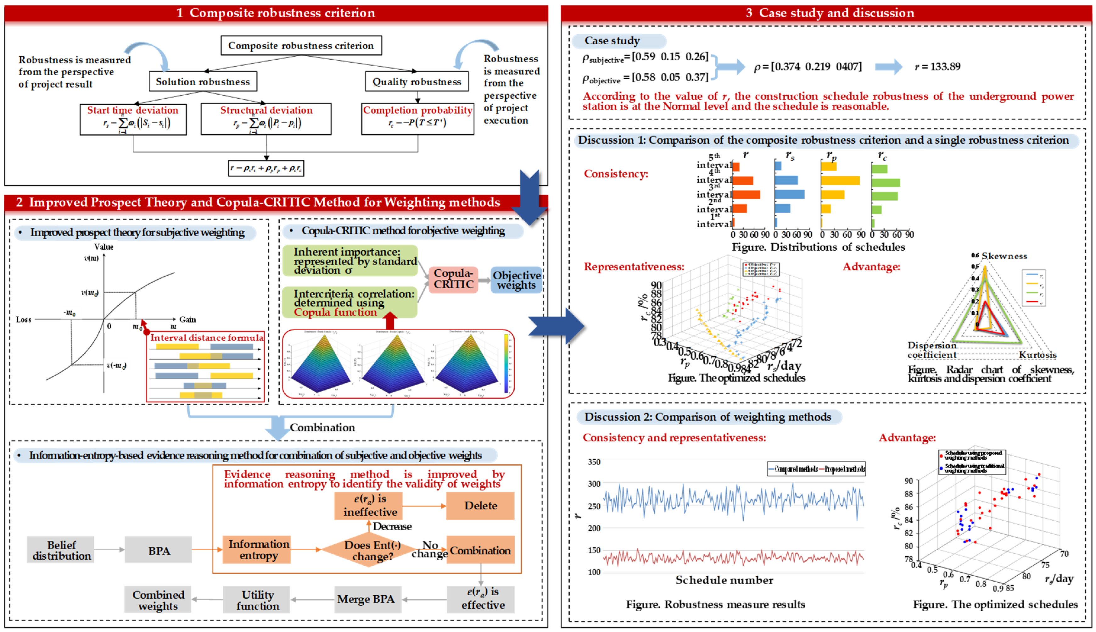
4.1. Composite Robustness Criterion

For real-life construction settings, activities and logic relationships among activities are two key components of a schedule, and construction duration is an important objective value of a schedule. Thus, it is meaningful to establish the robustness criterion from those three perspectives. Therefore, the composite robustness criterion includes start time deviation rs for measuring the schedule solution robustness via deviation between the actual start time and planned start time of each activity, structural deviation rp for measuring the schedule solution robustness via deviation between the actual construction order and planned construction order of each activity, and completion probability rc for measuring the schedule quality robustness via deviation of the construction duration, as shown in Equation (1):
r = ρ s r s + ρ p r p + ρ c r c
where rs is the absolute value of the weighted summation of the deviations between the activity’s actual start time and planned start time, i.e.,
r s = i = 1 n ω i ( | S i s i | )
where iN+ is the number of activities, ω i denotes the weight of activity i and is the normalized value of the additional cost corresponding to the activity i, Si represents the actual start time of activity i and si represents the planned start time of activity i, the unit of which is days.
In Equation (1), rp is the absolute value of the weighted summation of the deviations between the activity’s actual construction order and planned construction order, i.e.,
r p = i = 1 n ω i ( | P i p i | )
where Pi and pi are the actual and planned order of activity i respectively, which are dimensionless. Pi is determined by discrete event simulation [1], pi is determined according to the design of the construction manager.
In Equation (1), rc is the contrary number of a schedule’s completion probability, i.e.,
r c = P ( T T )
where T and T’ are the actual and planned construction duration, the unit of which is days. P represents probability. A schedule’s completion probability is determined as P(TT’) [10]. A bigger completion probability indicates better quality robustness of a construction schedule. Nevertheless, smaller rs and rp indicate better solution robustness of a construction schedule. Since it is necessary to keep the monotonicity of the rs, rp, and rc consistent, rc should be the contrary number of P(TT’), as shown in Equation (4).
In Equation (1), ρ s , ρ p and ρ c are the weights of rs, rp, and rc, whose detailed calculation methods are illustrated in Section 4.2, Section 4.3 and Section 4.4.

4.2. Improved Prospect Theory for Subjective Weighting

Improved prospect theory is proposed to determine the subjective weights. To overcome the shortcoming that the subjective weights given by experts are rationally bounded because of the experts’ individual preferences, the experts’ individual preferences are calculated and eliminated by prospect theory. In this way, the subjective weights of the bounded rationality can be transformed into subjective weights of rationality. Meanwhile, the interval distance formula is introduced into the prospect theory to overcome the shortcoming that prospect theory cannot deal with complete expert evaluation information. The procedure of subjective weighing is as follows:
  • Obtain the interval-valued weights of rs, rp and rc given by n experts (as shown in Table 1).
  • Determine the reference intervals of the three robustness criteria by the arithmetic mean method:
    v p s = f ( ρ s 1 sub , ρ s 2 sub , , ρ s n sub )   v p p = f ( ρ p 1 sub , ρ p 2 sub , , ρ p n sub )   v p c = f ( ρ c 1 sub , ρ c 2 sub , , ρ c n sub )
    where, vps, vpp and vpc represent the reference intervals. f ( · ) is the arithmetic mean function.
  • Establish the matrix of reference intervals VP:
    VP = [vps, vpp, vpc]
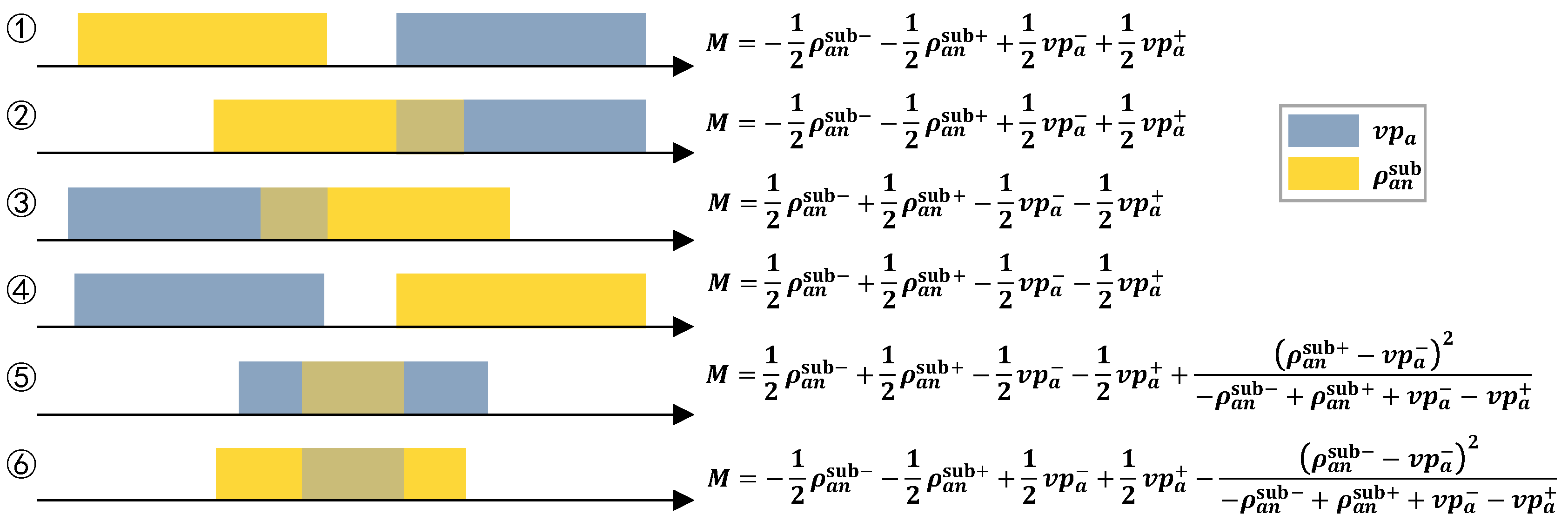
  • Obtain the gain/loss matrix M, which is the matrix reflecting experts’ individual preference. Gain implies that the subjective weight given by the expert is larger than RP. Loss implies that the subjective weight given by the expert is smaller than RP. M is computed using interval distance formula, i.e.,
    M = m ( v p a , ρ a n sub ) = 0 1 | [ v p a + x ( v p a + v p a ) ] [ ρ a n sub + x ( ρ a n sub + ρ a n sub ) ] | d x = 0 1 | ( v p a ρ a n sub ) + ( v p a + v p a + + ρ a n sub ρ a n sub + ) x | d x  
    where a = s , p , c represents the three robustness criteria, ρ a n sub is the subjective weights given by experts, m ( v p a , ρ a n sub ) is the distance between vpa and ρ a n sub . m ( v p a , ρ a n sub ) is calculated as follows: take the weighted absolute value of the left and right endpoint values of two intervals, then the value is traversed in [0, 1] and the combined result is the distance between the intervals.
    There are six kinds of positional relationships between v p a and ρ a n sub . The positional relationships and the corresponding distance formulas derived from Equation (7) are shown in Figure 2.
  • Calculate the value function through M = m(vpa, ρ a n sub ). The value function is the function reflecting the value of weights given by experts, with the gain/loss as an independent variable and the value of weights given by experts as a dependent variable. It is calculated as
    v ( m ) = { m α m 0 λ ( m ) β m < 0
    where v ( · ) is the value function, α is the positive risk attitude coefficient, while β is the negative risk attitude coefficient, and 0 α ,     β 1 . λ is the loss avoidance coefficient. It is suggested that α = 0.89 , β = 0.92 and λ = 2.25 [46].
  • Calculate the comprehensive prospect value:
    V = π ( V P ) · v ( m )
    where π ( V P ) is the weight function and weights of different experts are assigned identically.
  • Finally, the subjective weights, considering bounded rationality can be calculated:
    ρ subjective - a = v ( m ) V .

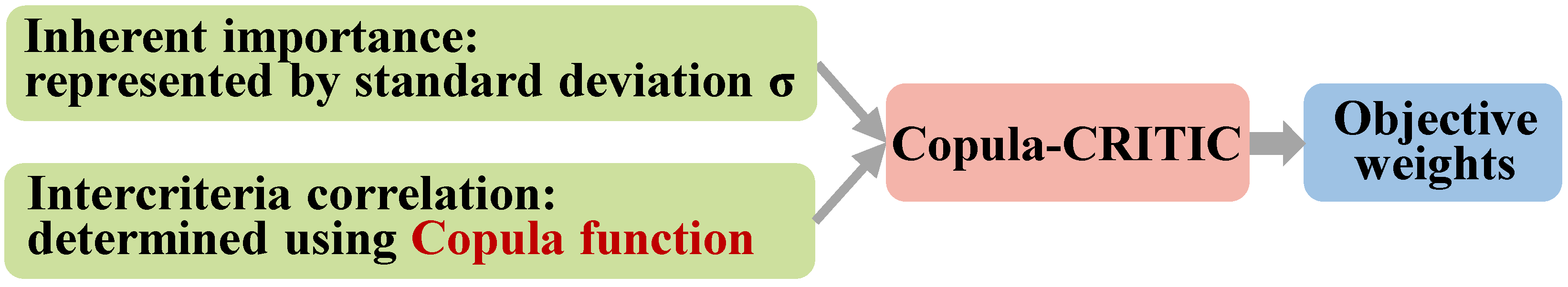
4.3. Copula-CRITIC Method for Objective Weighting

The Copula-CRITIC method is proposed to determine the objective weights. To overcome the shortcoming that the Pearson correlation coefficient function in the CRITIC method cannot effectively deal with, i.e., the difficulty in the intercriteria correlation among the three robustness criteria, the Copula function is introduced into the CRITIC method to replace the Pearson correlation coefficient function. In this way, the nonlinear correlation among rs, rp, and rc can be obtained, and the objective weights incorporating both inherent importance and nonlinear intercriteria correlations can be obtained (as shown in Figure 3).
The procedure of objective weighing is as follows:
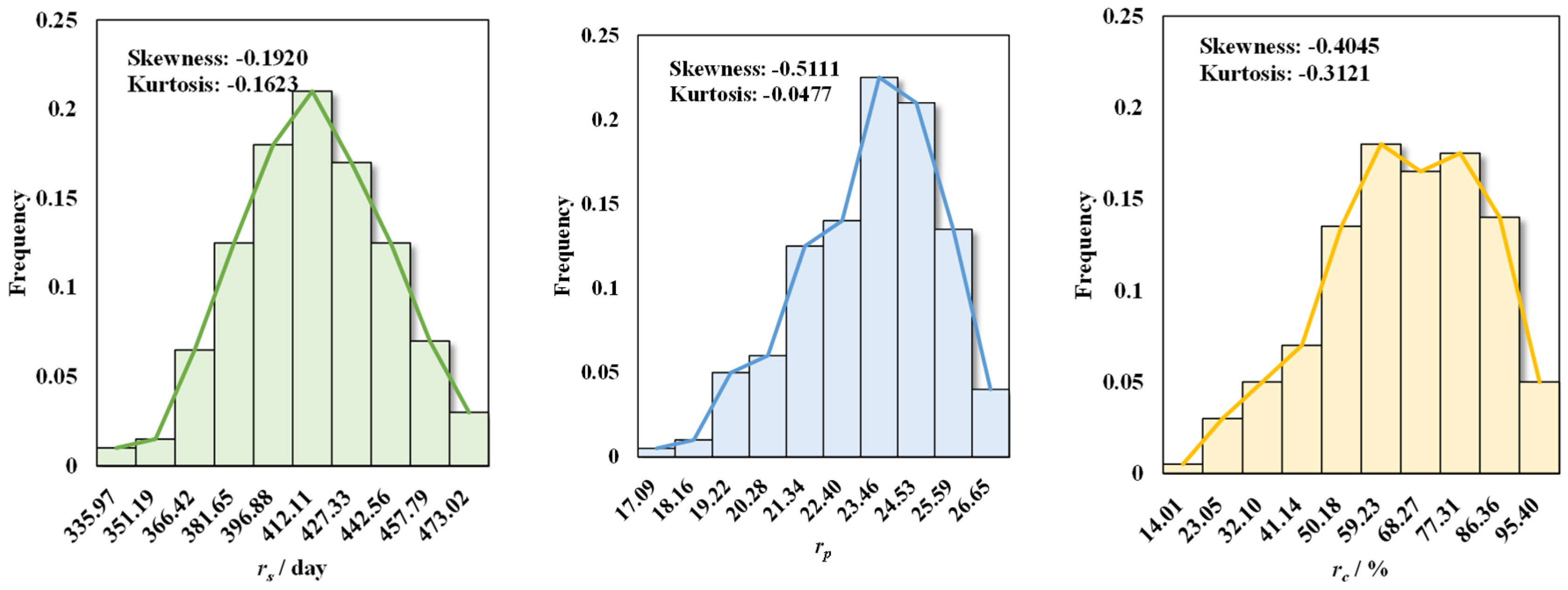
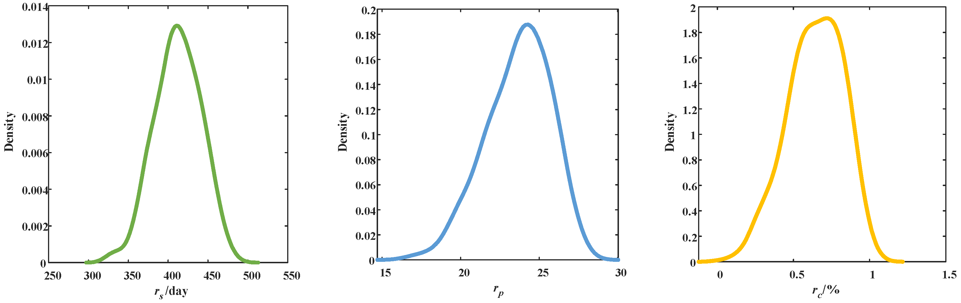
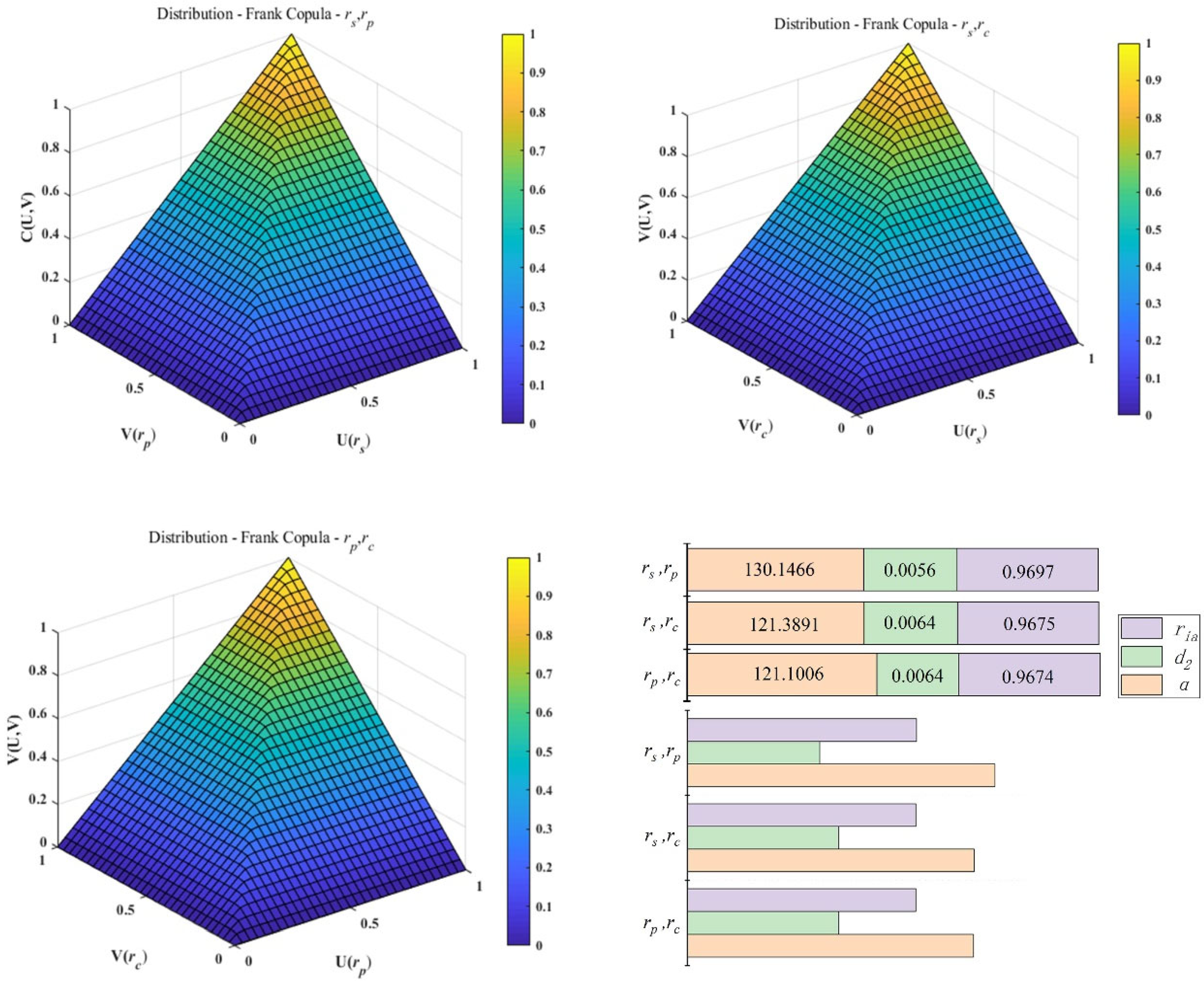
  • By using the Copula-CRITIC method, the objective weights are determined according to the inherent importance and nonlinear intercriteria correlation of three robustness criteria. Set Ca as the information contained in ra (a = s, p, c), Ca is
    C a = σ a i = s c ( 1 l i a )
    where C a represents the criterion’s information, σ a is the standard deviation to represent its inherent importance, and l i a is the correlation coefficient and is computed using the Copula function.
  • Compute l i a using the Copula function: Five classical Copula functions [47] are applied to the distribution fitting of the robustness criteria. The unknown parameters in the five Copula functions are determined by semi-parameter estimations. Then, the best Copula function is chosen according to the squared Euclidean distance d2 between the fitting Copula function and the empirical Copula function. The smaller d2 is, the better the fitting degree is. The d2 is calculated as follows:
    d 2 = a = s c | C ( r s , r p , r c ) C ( r s , r p , r c ) | 2
    where C ( r s , r p , r c ) represents the empirical Copula function, and C ( r s , r p , r c ) represents the fitting Copula function.
  • Calculate the objective weights ρobjective: Considering the standard deviations σ a and the correlation coefficients l i a , the objective weights of each criterion can be calculated:
    ρ objective - a = C a / a = s a ( C a )   ( a = s , p , c ) .

4.4. Information-Entropy-Based Evidence Reasoning Method for the Combination of Subjective and Objective Weights

In order to exclude invalid information from the weight combination process, the evidence reasoning method is improved by introducing the information-entropy-based effectiveness validation mechanism in the initial weight assignment stage in this paper, making the robustness measure a better reflection of bounded rational of subjective weights, inherent importance and interrelationships of objective weights [48]. The procedure of combination of subjective and objective weights is as follows:
  • Define H. H is the acceptance degree of ρ subjective and ρ objective . It has five classifications {SN, N, A, Y, SY}, which correspond to {Strongly no, No, Accept, Yes, Strongly yes}. Their utility values are U(SN) = −1, U(N) = −0.5, U(A) = 0, U(Y) = 0.5, U(SY) = 1. The belief distribution of the robustness criterion ra to weight ρ b ( b = subjective , objective ) is:
    S ( ρ b ( r a ) ) = { ( H x , θ x , b ( r a ) ) , x H ; ( H , θ H , b ( r a ) ) } .
  • Compute BPA. Basic probability assignment (BPA) e represents the accepted probability of ρ b with H. The belief distribution S ( ρ b ( r a ) ) is transformed to BPA by Equations (15)–(18).
    e x , b = e b ( H x ) = 0.5 θ x , b ( r a )
    e H , b = e b ( H ) = 1 x = S N S Y e H , b = 1 0.5 x = S N S Y θ x , b ( r a )
    e ¯ H , b = e ¯ b ( H ) = 1 0.5 = 0.5
    e H , b = e b ( H ) = 0.5 ( 1 x = S N S Y e H , b )
    where e x , b is the BPA of the total weight to ρ b with the acceptation degree of H x , eH, b is the BPA of the total weight to ρ b with all acceptation degrees. e H , b = e ¯ H , b + e H , b . e ¯ H , b appeared as the result of other weights, and e H , b appeared as the result of the unascertained acceptance degrees.
  • Merge the basic probabilities of subjective and objective weights:
    e ( r a ) = ( e 1 e 5 ) ( r a ) = e r a b = subjective objective e x ( r a ) K
    where K is the orthogonalized constant, representing the combination degree of different probabilities, which is calculated as
    K = e b = subjective objective e x ( r a ) .
  • Validate the effectiveness of weights. The effectiveness is validated by calculating the change in entropy during step 3 (as shown in Equation (21)). A decrease in entropy suggests that the merged weights are valid; otherwise, the weight is invalid and should be deleted during step 3.
    E n t ( r a ) = e ( r a ) log 2 ( r a )
  • Calculate the probabilities that ρ b is accepted with H x and H are calculated:
    θ x = e x 1 e ¯ H ,
    θ H = e H 1 e ¯ H .
  • Calculate the utility of the robustness criterion. The utility function is shown in Equation (24). Thus, the minimum utility U min , maximum utility U max , and average utility U avg can be obtained:
    U = θ x U ( H x )
    U max = ( θ 1 ( r a ) + θ H ( r a ) ) U ( H 1 ) + x = 2 5 ( θ x ( r a ) U ( H x ) )
    U min = ( θ N ( r a ) + θ H ( r a ) ) U ( H N ) + x = 1 4 ( θ x ( r a ) U ( H N ) )
    U avg = U max + U min 2 .
  • The total weight of robustness criterion can be obtained:
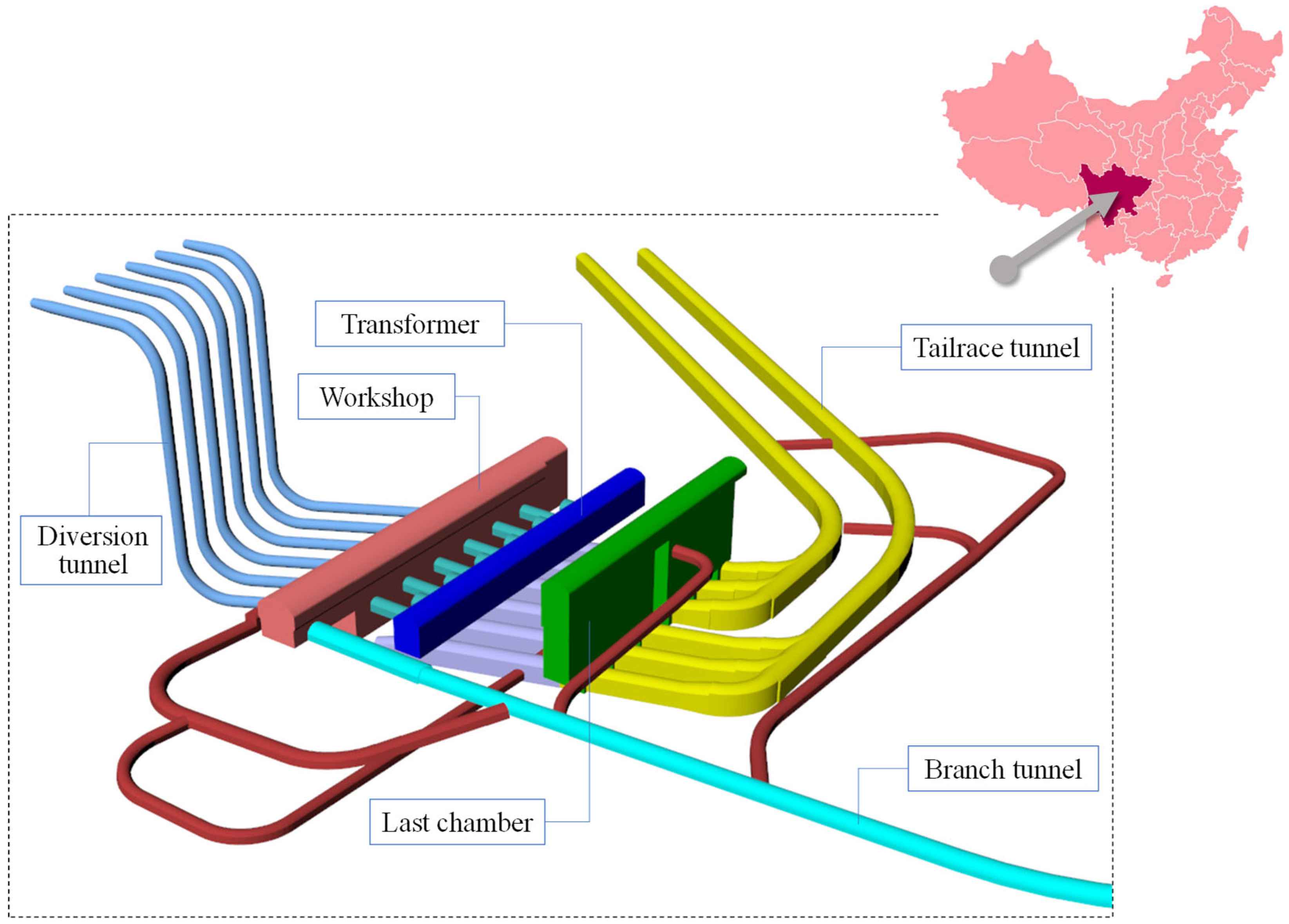
    ρ a = U avg , a / a = s a ( U avg , a ) .

5. Case Study

An underground power station in China is used for a case study. Its construction schedule robustness is measured using the composite robustness criterion and weighting methods proposed in this paper. The criterion’s subjective, objective, and combined weights are calculated, and rs, rp, rc of the project are determined. Then, the composite robustness criterion of the underground power station’s construction schedule is obtained.

5.1. Project Overview

The underground power station used as a case study is in Southwest China. As shown in Figure 4, it is composed of the main workshop, main transformer, last chamber, and several branch tunnels.

5.2. Weighting of Robustness Criteria

5.2.1. Subjective Weighting

The subjective weights are determined. Taking underground power stations as an example, experts’ judgments on the mechanical malfunction probability of different machines are not identical to the expected utility curve. Although hand drills often fail, the malfunction rate given by experts is lower than the actual statistical results due to their low price. On the contrary, though three-arm trolleys have low failure frequency, their failure rate provided by experts is higher than the actual statistical results because of their high costs [49]. Thus, prospect theory is adopted and improved to calculate the subjective weights.
The evaluation results given by ten experts are shown in Table 2, where RPs are calculated. It can be known that the subjective weighting method adapted with improved prospect theory is capable of handling interval-valued weights.
The gain/loss matrix M and value function matrix are obtained:
M = [ 0.1100 0.1050 0.0350 0.0125 0.0550 0.0694 0.0900 0.0950 0.1150 0.0400 0.0450 0.0150 0.0400 0.1050 0.0850 0.0600 0.0450 0.0386 0.0900 0.1450 0.0150 0.0600 0.0634 0.1850 0.1100 0.0228 0.0150 0.0900 0.0277 0.1150 ] ,   v = [ 0.1402 0.2829 0.0506 0.0202 0.1561 0.0931 0.2455 0.1231 0.3076 0.1164 0.0633 0.0472 0.1164 0.2829 0.1115 0.0818 0.0633 0.0553 0.2455 0.1793 0.0472 0.0818 0.0859 0.2227 0.1402 0.0345 0.0472 0.2455 0.0411 0.3076 ]
Based on the value function matrix above, the comprehensive prospect value is obtained:
V = [ 1 1 1 1 1 1 1 1 1 1 ] T × [ 0.1402 0.2829 0.0506 0.0202 0.1561 0.0931 0.2455 0.1231 0.3076 0.1164 0.0633 0.0472 0.1164 0.2829 0.1115 0.0818 0.0633 0.0553 0.2455 0.1793 0.0472 0.0818 0.0859 0.2227 0.1402 0.0345 0.0472 0.2455 0.0411 0.3076 ] = [ 0.5052 0.1314 0.2237 ]
Here the subjective weights of each criterion, considering bounded rationality, can be gained according to the value function and the comprehensive prospect value:
ρ subjective = [ 0.59 0.15 0.26 ]

5.2.2. Objective Weighting

The objective weights are determined. Nonlinear intercriteria correlations among rs, rp, and rc, are calculated using the Copula function. A total of 200 schedules are generated, and their rs, rp, and rc are calculated. Their frequency distributions, including skewness and kurtosis, are shown in Figure 5.
Figure 5 indicates that the frequency distribution curves of the three robustness criteria do not obey normal, Poisson, and other basic distributions. Thus, the distribution function of the three criteria is fitted, which are shown in Figure 6.
Then, the results above are applied to the five Copula functions to estimate the unknown parameters of each function by using the maximum likelihood method. The results are shown in Table 3.
The squared Euclidean distances d2 between the empirical Copula function and the five classical Copula functions are calculated, as shown in Table 4.
It can be seen from Table 4 that the d2 between the empirical Copula function and the Frank Copula function is the smallest, which suggests that the Frank Copula function fits best. Thus, the Frank Copula function was adopted to calculate the nonlinear intercriteria correlations among robustness criteria. Figure 7 illustrates the Frank Copula functions and their comparisons with the empirical Copula function.
The parameter estimation results in Table 3 are applied to the Frank Copula function, and the rank correlation coefficients can be obtained: ls-p = 0.9697, ls-c = 0.9675, lp-c = 0.9674. In addition, the standard variance reflecting the self-strength of the different criteria are σ s = 28.61 , σ p = 2.02 , σ c = 17.80 .
Here the objective weights of each criterion, which could incorporate both inherent importance and nonlinear intercriteria correlations, can be gained:
ρ objective = [ 0.58 0.05 0.37 ]

5.2.3. Combination of Subjective and Objective Weights

Thirdly, the subjective and objective weights are combined. The belief distribution of the subjective and objective weights of rs, rp, and rc is shown in Table 5.
The contents of Table 5 are then transformed to BPA, as shown in Table 6.
The BPAs are merged and the weight distributions are calculated, as shown in Table 7.
At last, the combined weights are obtained:
ρ = [ 0.374 0.219 0.407 ]

5.3. Measure Results

According to Section 4.2, the composite robustness criterion of the construction schedule can be obtained as: r = 0.374 r s + 0.219 r p + 0.407 r c . Meanwhile, the three robustness criteria of this project can, respectively, be calculated as follows:
r s = i = 1 n ω i ( | S i s i | ) = 0.0173 × | 121 138 | + 0.0173 × | 179 183 | + 0.0119 × | 237 243 | + = 419.31       ↑       ↑       ↑   main   transformer   main   transformer   main   transformer       hall   layer   # 2 - 1   hall   layer   # 2 - 2   hall   layer   # 3
r p = i = 1 n ω i ( | P i p i | ) = 0.0173 × | 7 7 | + 0.0173 × | 11 12 | + 0.0119 × | 12 15 | + = 21.64       ↑       ↑       ↑   main   transformer   main   transformer   main   transformer       hall   layer   # 2 - 1   hall   layer   # 2 - 2   hall   layer   # 3
r c = P ( T T ) = P ( T 2043 ) = 67.98
So, the composite robustness criterion of this project is r = 133.89. The range of r is [0, 275] and the schedule robustness is divided into five levels according to the contribution of criterion r change to schedule robustness: the schedule robustness is Very good when 0 ≤ r < 55, the schedule robustness is Good when 55 ≤ r < 110, the schedule robustness is Normal when 110 ≤ r < 165, the schedule robustness is Bad when 165 ≤ r < 220, and the schedule robustness is Very bad when 220 ≤ r < 275. Thus, r = 133.89 means the schedule robustness of the underground power station is at the Normal level and the schedule is reasonable.

6. Discussion

The measured results of the proposed criterion and methods are compared with the results using either the solution robustness or the quality solution, and the results using the composite criterion based on traditional weighting methods including AHP for subjective weighting [23], entropy weighting method for objective weighting [36] and geometric mean method for combining weights [40]. Thus, the consistency, representativeness, and advantage of the proposed criterion and methods are verified.

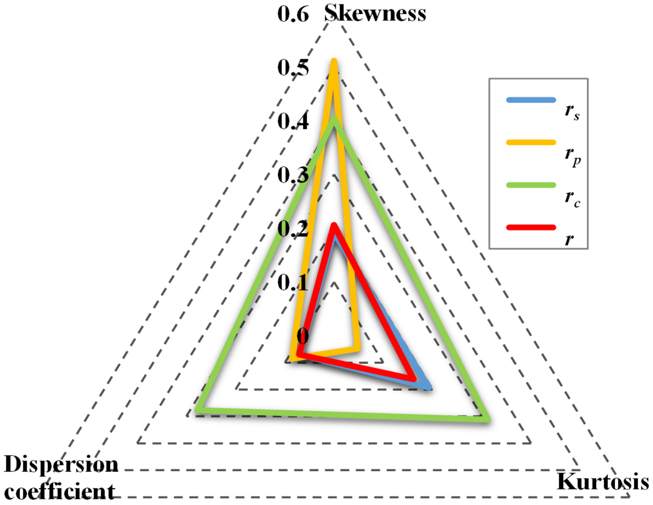
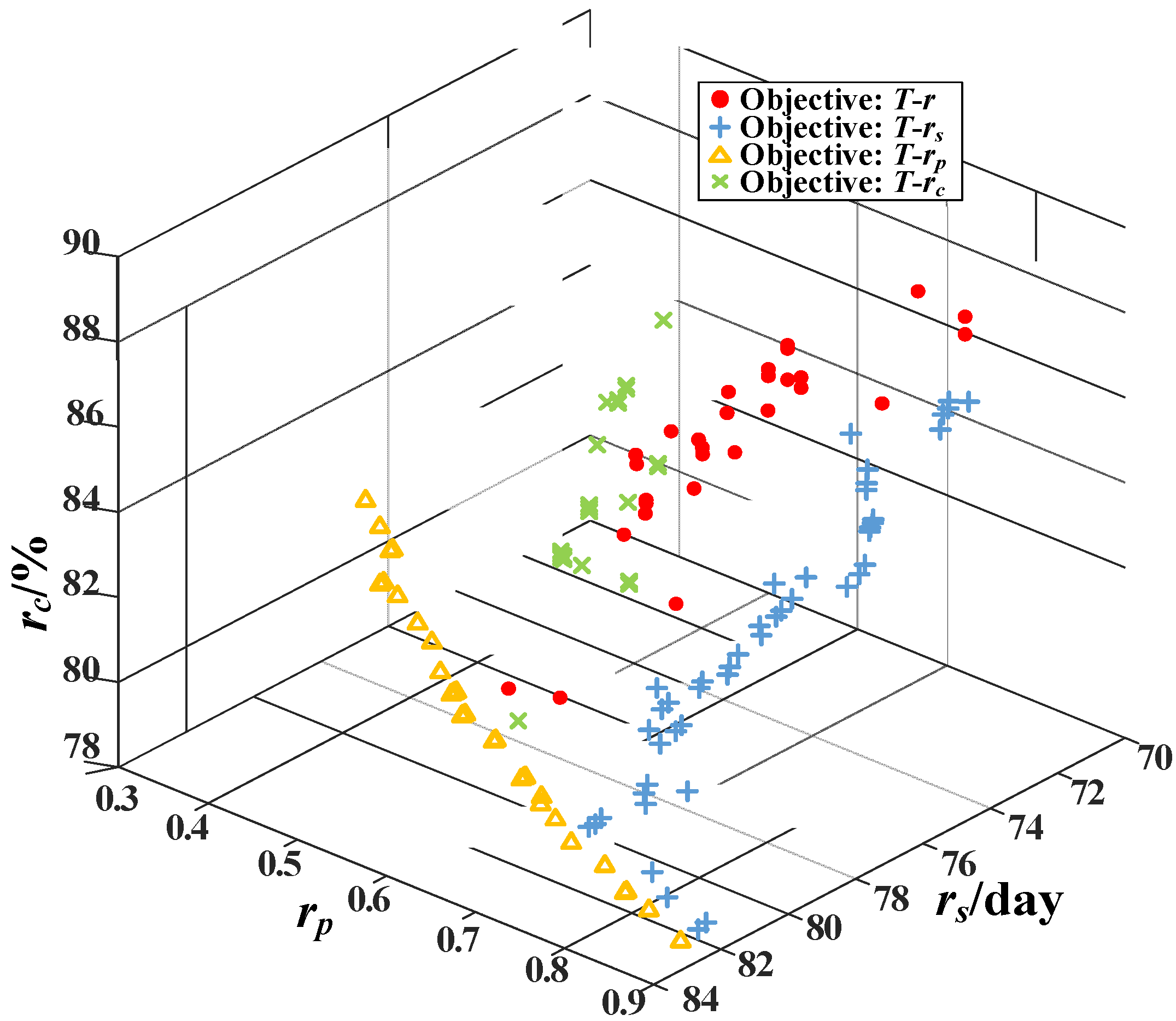
6.1. Comparison of the Composite Robustness Criterion and a Single Robustness Criterion

A total of 200 schedules meeting the logical relationship and resource restrictions of this project are generated randomly and their composite robustness criterion r and three single robustness criteria rs, rp, and rc are calculated.
The measured results are divided into five intervals on average. The quantity of schedules that belongs to each interval is shown in Figure 8. The robustness of these schedules measured via r are mainly within the third and fourth intervals, and a few ones are in the second and fifth intervals, and the schedules in the first interval are the least. This phenomenon complies with the circumstances of the measured results of rs, rp, and rc. Therefore, the robustness measured result of r is consistent with the results of existing single criteria.
In order to analyze the representativeness of the proposed composite robustness criterion, which is embodied by the symmetry, concentration, and even dispersion of r as well as rs, rp, and rc, the skewness, kurtosis and dispersion coefficient of the measured results are calculated. As shown in Figure 9, the kurtosis of rs and rc is rather high, which suggests a strong concentration, and thus extreme and invalid evaluations in measuring robustness. The skewness of rp is very high, which suggests an obvious negative skewness, and its accuracy would be low when measuring the schedule robustness whose fluctuation in structural robustness and quality robustness is small. The dispersion coefficient of rc is rather large, which suggests poor criterion representativeness, and it would be useless when used individually. From the comparison, it can be drawn that the composite robustness criterion r has desirable symmetry, concentration, and uniform dispersion, which balances the three single criteria and is representative in robustness measure of the construction schedule.
To verify the advantage of the proposed composite robustness criterion, the optimization of construction duration and schedule robustness is conducted. Construction duration T and schedule robustness, which is measured using r, rs, rp, and rc, respectively, are the two optimization objectives. A hybrid grey wolf optimizer with a sine-cosine algorithm is adopted to solve the optimization model [50]. The iteration number is set as 1000. The optimization results in Figure 10 show that when the optimization environment is the same, and optimized duration level is equal, the optimized schedules with the objectives of T-rs (or T-rp, T-rc) only have good solution robustness or good quality robustness, but do not have robustness in both aspects. The optimized schedules with the objectives of T-r have both good solution robustness and good quality robustness, which ensures the schedules’ anti-interference ability from the perspectives of both project execution and project result. Therefore, the composite robustness criterion r proposed in this paper has the advantages of comprehensively measuring the robustness, in terms of both project execution and project result.

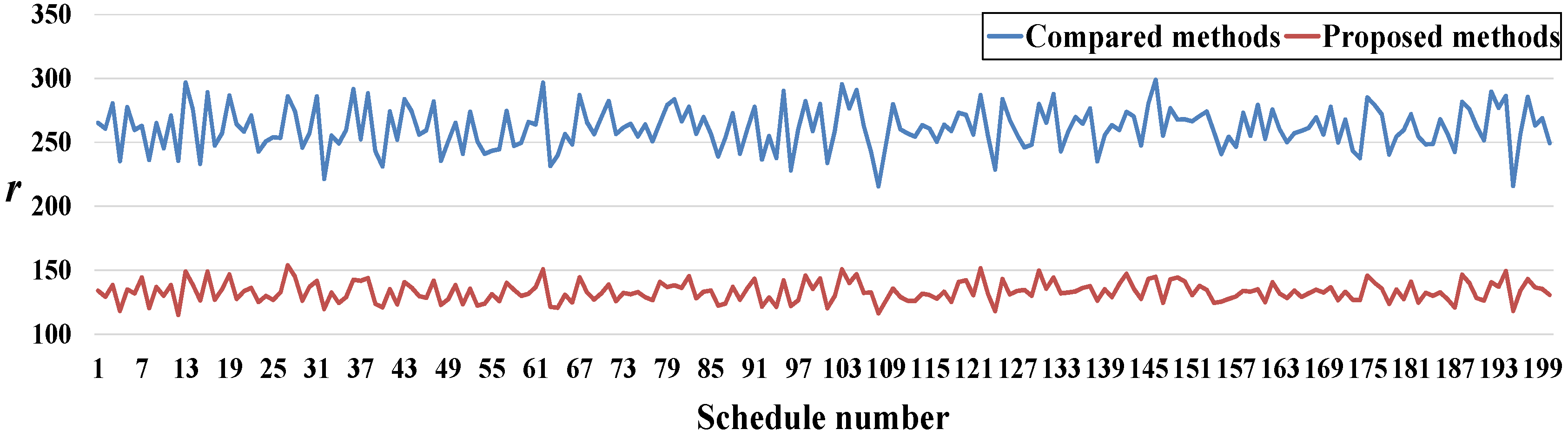
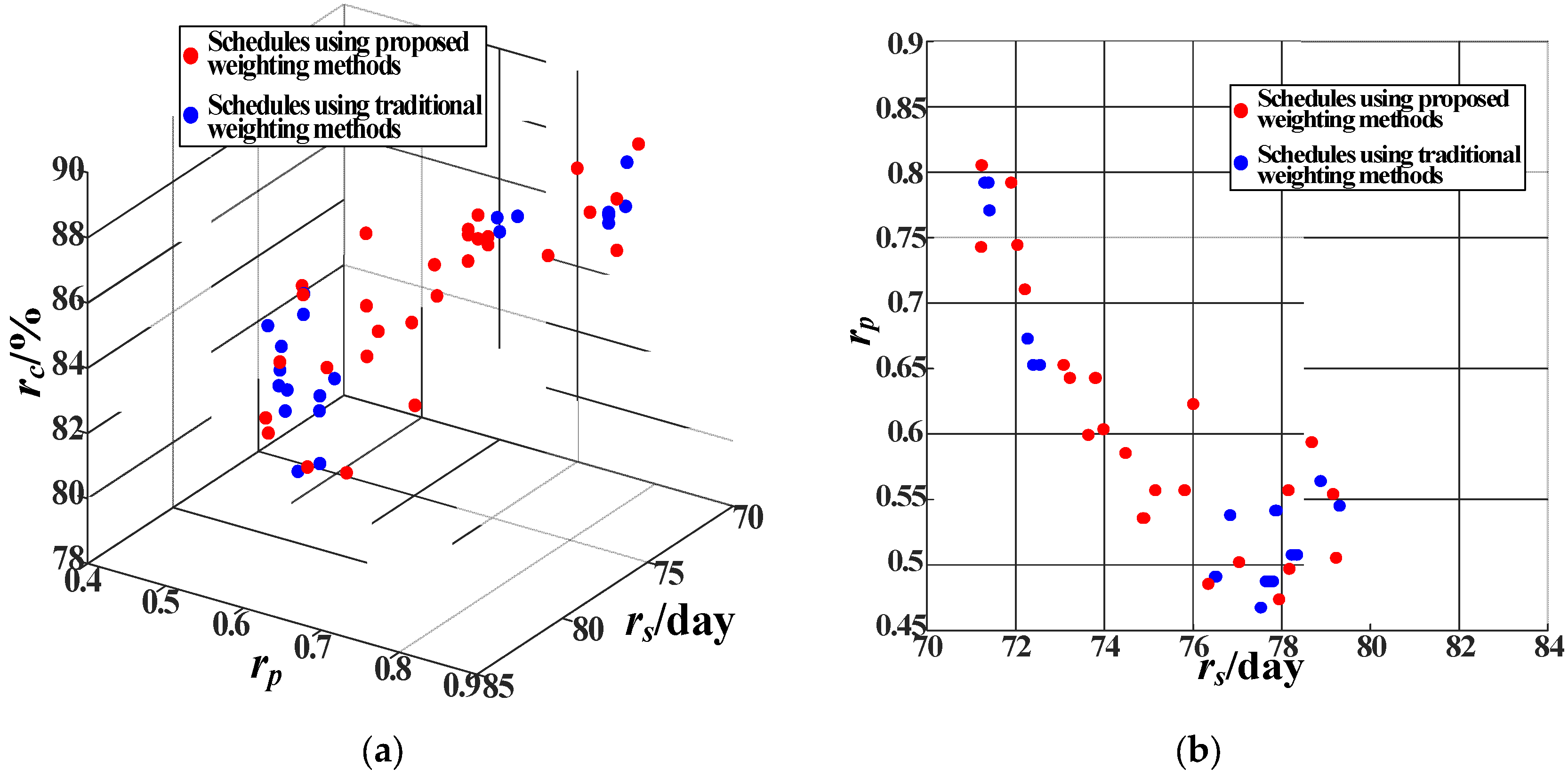
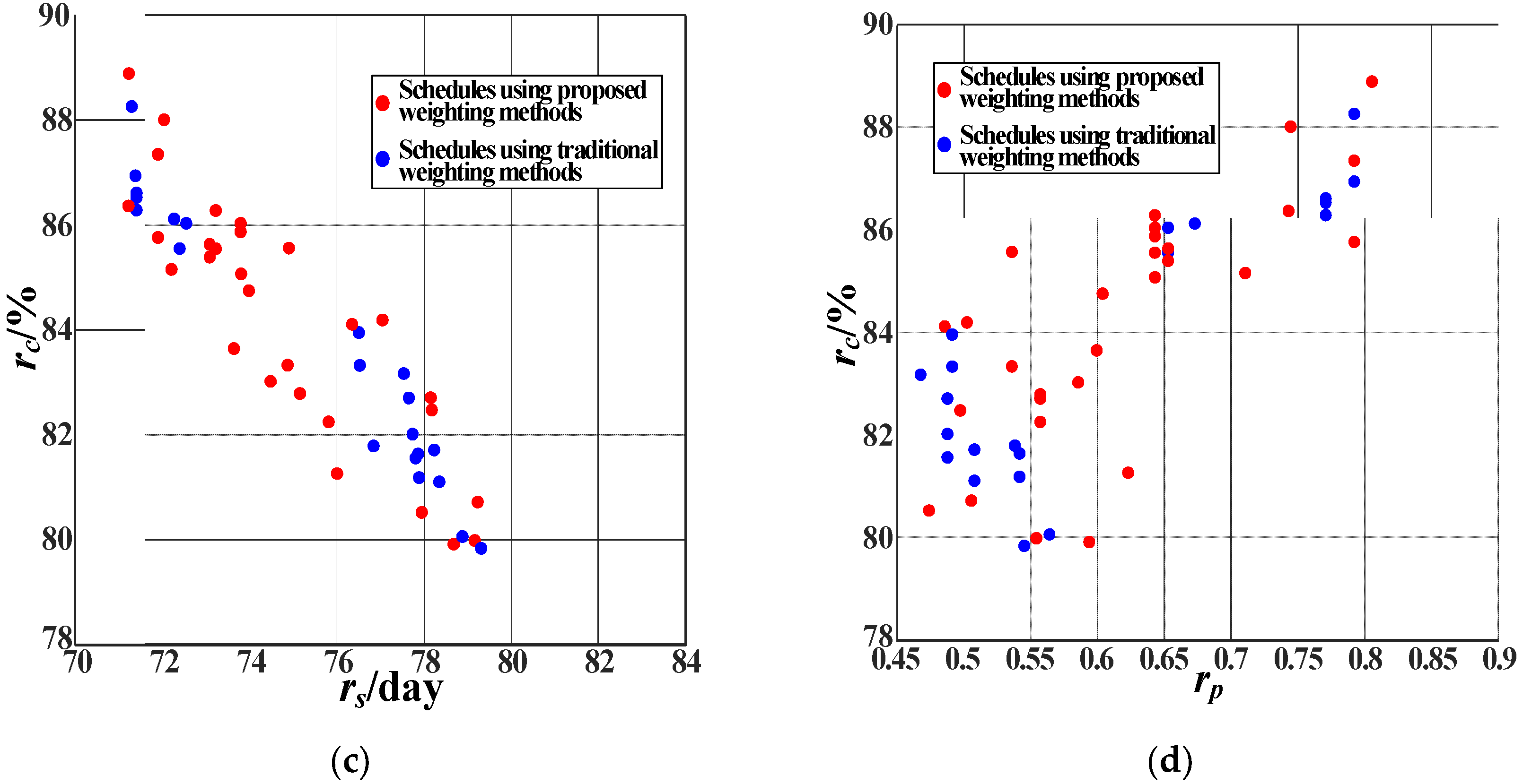
6.2. Comparison of Weighting Methods

The robustness measure of the current project can be r = 0.669 r s + 0.080 r p + 0.251 r c , where the subjective weights are determined by AHP, the objective weights are calculated by entropy weighting method, and the two weights are combined by the geometric mean method. The methods proposed as well, as the traditional methods mentioned above, were respectively applied to measure the robustness of the 200 schedules. The results are shown in Figure 11. Line chart trends of the two sets of methods are obviously consistent, thus suggesting the consistency of the proposed weighting methods in measuring robustness.
In addition, the standard deviation of r with the proposed weighting methods is 7.89, while using the traditional weighting methods is 16.49. Thus, the robustness measure results using the proposed weighting methods have lower dispersion degree, suggesting their representativeness.
Then, the optimization of construction duration and schedule robustness is conducted to verify the advantage of the proposed weighting methods. Construction duration T and schedule robustness, which is measured using the composite robustness criterion using the weighting methods proposed in this paper and the traditional weighting methods, respectively, are the two optimization objectives. A hybrid grey wolf optimizer with a sine-cosine algorithm is adopted to solve the optimization model [50]. The iteration number is set as 1000. The optimization results in Figure 12 show that the optimized schedules with the objectives of T and r obtained using the proposed weighting methods are evenly distributed on the whole Pareto front, while the optimized schedules with the objectives of T and r obtained using the traditional weighting methods are distributed at the two ends of the Pareto front, lacking schedules with good start time deviation, good structural deviation, and good completion probability at the same time. Thus, the proposed weighting methods have the advantage of letting the robustness information of the composite criterion be completely expressed.

7. Conclusions

The robustness measure of a construction schedule is an effective and indispensable tool to evaluate the capability of robust scheduling. However, current research mainly pays pay to a single robustness criterion. Few studies consider both the solution robustness and quality robustness while neglecting the bounded rationality of subjective weights and the inherent importance and nonlinear intercriteria correlations of objective weights in the composite criterion. In view of these limitations, a construction schedule robustness measure based on improved prospect theory and the Copula-CRITIC method is proposed in this paper. An underground power station in China was used as a case study to verify its advantages. The main contributions of this paper are listed as follows:
  • With the establishment of a composite robustness criterion containing solution robustness criteria of start time deviation and structural deviation, and quality robustness criterion of completion probability, construction schedule robustness can be measured in terms of both project execution and project result.
  • The subjective weights considering bounded rationality are assigned using prospect theory improved by an interval distance formula, the objective weights taking both inherent importance and nonlinear intercriteria correlations into account are assigned using the Copula-CRITIC method, and the subjective and objective weights are combined using an information-entropy-based evidence reasoning method.
  • A real underground power station was used as a case study. The results of the proposed criterion and methods, one with a single robustness criterion of either solution robustness or quality robustness, and one with a composite robustness criterion using a traditional weighting method were compared to verify the consistency, representativeness, and advantages of the proposed composite robust criterion and weighting methods.

Author Contributions

Conceptualization, X.W. and M.Z.; methodology, M.Z.; software, M.Z.; validation, M.Z., and J.Y.; investigation, M.Z. and L.X.; data curation, L.X. and S.Y.; writing—original draft preparation, M.Z.; writing—review and editing, J.Y. and S.Y. All authors have read and agreed to the published version of the manuscript.

Funding

This research was funded by the National Natural Science Foundation of China, grant number 51679165; the Yalong River Joint Funds of the National Natural Science Foundation of China, grant number U1965207; and the National Natural Science Foundation of China, grant number 51839007.

Conflicts of Interest

The authors declare no conflict of interest.

Nomenclature

SymbolDefinitionSymbolDefinition
rComposite robustness criterionπ(VP)Weight function in prospect theory
rsRobustness criterion, start time deviationρsubjective-aSubjective weight of robustness criterion
rpRobustness criterion, structural deviationρobjective-aObjective weight of robustness criterion
rcRobustness criterion, completion probabilityCaIntermediate variable containing information of robustness criterion in Copula-CRITIC method
ρaWeight of robustness criterion, a=s, p, c σ a Standard deviation
iActivity number, IN+li-aCorrelation coefficient among robustness criteria
ωiWeight of activity i C ( r s , r p , r c ) Empirical Copula function
SiActual start time of activity i C ( r s , r p , r c ) Fitting Copula function
siPlanned start time of activity id2Square Euclidean distance between C ( r s , r p , r c ) and C ( r s , r p , r c )
PiActual construction order activity iHAcceptation degree of ρ subjective and ρ objective
piPlanned construction order activity iU(·)Utility function of H
TActual construction durationS(ρa(ra))Belief distribution of ρa to ra
T’Planned construction durationeBasic probability assignment (BPA)
EnExpertex, bBPA of total weight to ρ b with the acceptation degree of H x
ρ a n sub Subjective weights given by expertseH, bBPA of total weight to ρ b with all acceptation degrees
v ρ a n sub Reference interval e ¯ H , b eH, b‘s result of other weights
VPMatrix of the reference interval e H , b eH, b‘s result of the unascertained acceptation degrees
MGain/loss matrixKOrthogonalized constant, represent the combination degree of different probabilities
m ( v p a , ρ a n sub ) Entries in matrix M, the distance between v p a and ρ a n sub Ent(·)Entropy, represent the effectiveness of weight
v(m)Value functionθxProbability that ρ b is accepted with H x
α Positive risk attitude coefficient, α = 0.89 θHProbability that ρ b is accepted with H
β Negative risk attitude coefficient, β = 0.92 UminMinimum utility
λ Loss avoidance coefficient, λ = 2.25 UmaxMaximum utility
VComprehensive prospect valueUavgAverage utility

References

  1. Stijn, V.d.V. Proactive-Reactive Procedures for Robust Project Scheduling. Ph.D. Thesis, University of Leuven, Leuven, Belgium, 2006. [Google Scholar]
  2. Lambrechts, O.; Demeulemeester, E.; Herroelen, W. Time slack-based techniques for robust project scheduling subject to resource uncertainty. Ann. Oper. Res. 2011, 186, 443–464. [Google Scholar] [CrossRef]
  3. Akkan, C. Improving schedule stability in single-machine rescheduling for new operation insertion. Comput. Oper. Res. 2015, 64, 198–209. [Google Scholar] [CrossRef]
  4. Sundström, N.; Wigström, O.; Lennartson, B. Conflict between energy, stability, and robustness in production schedules. IEEE Trans. Autom. Sci. Eng. 2016, 14, 658–668. [Google Scholar] [CrossRef]
  5. Ansari, R.; Makui, A.; Ghoddousi, P. An algorithmic framework for improving the performance of the critical chain buffer sizing method. Sci. Iran. 2016, 25, 74–92. [Google Scholar] [CrossRef] [Green Version]
  6. Liu, F.; Wang, S.B.; Hong, Y.; Yue, X.H. On the robust and stable flowshop scheduling under stochastic and dynamic disruptions. IEEE Trans. Eng. Manag. 2017, 64, 539–553. [Google Scholar] [CrossRef]
  7. Xiao, S.C.; Sun, S.D.; Jin, J.H. Surrogate measures for the robust scheduling of stochastic job shop scheduling problems. Energies 2017, 10, 543. [Google Scholar] [CrossRef] [Green Version]
  8. Rahmani, D. A new proactive-reactive approach to hedge against uncertain processing times and unexpected machine failures in the two-machine flow shop scheduling problems. Sci. Iran. 2017, 24, 1571–1584. [Google Scholar] [CrossRef] [Green Version]
  9. Pang, N.S.; Su, H.F.; Shi, Y.L. Project robust scheduling based on the scattered buffer technology. Appl. Sci. 2018, 8, 541. [Google Scholar] [CrossRef] [Green Version]
  10. Zhong, D.H.; Bi, L.; Yu, J.; Zhao, M.Q. Robustness analysis of underground powerhouse construction simulation based on Markov Chain Monte Carlo method. Sci. China 2016, 59, 252–264. [Google Scholar] [CrossRef]
  11. Zhang, Y.; Cui, N.F.; Hu, X.J.; Hu, Z.T. Robust project scheduling integrated with materials ordering under activity duration uncertainty. J. Oper. Res.Soc. 2019, 3, 1–12. [Google Scholar] [CrossRef]
  12. Chang, Z.Q.; Ding, J.Y.; Song, S. Distributionally robust scheduling on parallel machines under moment uncertainty. Eur. J. Oper. Res. 2019, 272, 832–846. [Google Scholar] [CrossRef]
  13. Hu, C.; Lu, J.; Liu, X.; Zhang, G. Robust vehicle routing problem with hard time windows under demand and travel time uncertainty. Comput. Oper. Res. 2018, 94, 139–153. [Google Scholar] [CrossRef]
  14. Liang, Y.Y.; Cui, N.F.; Wang, T.; Demeulemeester, E. Robust resource-constrained max-NPV project scheduling with stochastic activity duration. Oper. Spectr. 2019, 41, 219–254. [Google Scholar] [CrossRef]
  15. Novianingsih, K.; Hadianti, R.; Uttunggadewa, S.; Soewono, E. Simulation for measuring the effect of flight retiming to the robustness of flight schedule. In Proceedings of the AIP Conference, Bandung, Indonesia, 8–9 November 2014. [Google Scholar]
  16. Hussain, T.S.; Richard, S.; Steve, R.S.; Nicole, O.; John, D.; John, C.; Julia, B.; Adan, E.V.; Allison, C. Robust and flexible air mobility scheduling using stochastic simulation-based assessment. In Proceedings of the 2015 WSC, Huntington Beach, CA, USA, 6–9 December 2015. [Google Scholar]
  17. Detti, P.; Nicosia, G.; Pacifici, A.; de Lare, G.Z.M. Robust single machine scheduling with a flexible maintenance activity. Comput. Oper. Res. 2019, 107, 19–31. [Google Scholar] [CrossRef]
  18. Lu, Z.Q.; Zhang, S.Y.; Cui, W.W. Integrating production scheduling and maintenance policy for robustness in flow shop problems. Acta Autom. Sin. 2015, 41, 906–913. [Google Scholar]
  19. Shen, X.N.; Han, Y.; Fu, J.Z. Robustness measures and robust scheduling for multi-objective stochastic flexible job shop scheduling problems. Soft Comput. 2016, 21, 1–24. [Google Scholar] [CrossRef]
  20. Lamas, P.; Demeulemeester, E. A purely proactive scheduling procedure for the resource-constrained project scheduling problem with stochastic activity durations. J. Sched. 2016, 19, 409–428. [Google Scholar] [CrossRef]
  21. Zhao, C.Y.; Lu, Z.Q.; Cui, W.W. Proactive scheduling optimization on flow shops with random machine breakdowns. J. Zhejiang Univ. 2016, 50, 641–649. [Google Scholar]
  22. Cui, W.; Lu, Z.; Li, C.; Han, X.L. A proactive approach to solve integrated production scheduling and maintenance planning problem in flow shops. Comput. Ind. Eng. 2018, 115, 342–353. [Google Scholar] [CrossRef]
  23. Joukar, A.; Nahmens, I.; Harvey, C. An AHP-based selection model for ranking potential strategies for managing construction’s cost volatilities. In Proceedings of the Construction Research Congress, San Juan, PR, USA, 31 May–2 June 2016. [Google Scholar]
  24. Cheshmidari, M.N.; Ardakani, A.H.H.; Alipor, H.; Shojaei, S. Applying Delphi method in prioritizing intensity of flooding in Ivar watershed in Iran. Spat. Inf. Res 2017, 25, 173–179. [Google Scholar] [CrossRef]
  25. Li, R.; Li, Y.; Xu, H.; Liu, H.T.; Miao, S.H.; Chen, J.; Cai, J. Assessment on typical power supply mode for important power consumers based on analytical hierarchy process and expert experience. Power Syst. Technol. 2014, 38, 2336–2341. [Google Scholar]
  26. Abdellaoui, M.; Han, B.; L’Haridon, O.; van Dolder, D. Measuring loss aversion under ambiguity: A METHOD to make prospect theory completely observable. J. Risk Uncertain. 2016, 52, 1–20. [Google Scholar] [CrossRef]
  27. Wang, M.; Zhao, K.; Zhu, Q.; Jiang, H.; Jin, J. Decision-making model of supporting schemes of foundation pit based on cumulative prospect theory and connection number. Rock Soil Mech. 2016, 37, 622–628. [Google Scholar]
  28. Bao, T.; Xie, X.; Long, P.; Wei, Z. MADM method based on prospect theory and evidential reasoning approach with unknown attribute weights under intuitionistic fuzzy environment. Expert Syst. Appl. 2017, 88, 305–317. [Google Scholar] [CrossRef]
  29. Jhala, K.; Natarajan, B.; Pahwa, A. Prospect theory-based active consumer behavior under variable electricity pricing. IEEE Trans. Smart Grid 2019, 10, 2809–2819. [Google Scholar] [CrossRef]
  30. Krcal, O.; Kvasnicka, M.; Stanek, R. External validity of prospect theory: The evidence from soccer betting. J. Behav. Exp. Econ. 2016, 65, 121–127. [Google Scholar] [CrossRef]
  31. Hens, T.; Mayer, J. Cumulative prospect theory and mean-variance analysis: A rigorous comparison. J. Comput. Financ. 2017, 21, 41–73. [Google Scholar] [CrossRef] [Green Version]
  32. Brunner, T.; Reiner, J.; Natter, M. Prospect theory in a dynamic game: Theory and evidence from online pay-per-bid auctions. Econ. Behav. Organ. 2019, 164, 215–234. [Google Scholar] [CrossRef]
  33. Zhang, Z.; Wang, L.; Rodriguez, R.M.; Wang, Y.; Martinez, L. A hesitant group emergency decision making method based on prospect theory. Complex Intell. Syst. 2017, 3, 177–187. [Google Scholar] [CrossRef]
  34. Liu, P.; Li, Y. An extended MULTIMOORA method for probabilistic linguistic multi-criteria group decision-making based on prospect theory. Comput. Ind. Eng. 2019, 136, 528–545. [Google Scholar] [CrossRef]
  35. Hackel, B.; Pfosser, S.; Trankler, T. Emergency alternative evaluation using extended trapezoidal intuitionistic fuzzy thermodynamic approach with prospect theory. Int. J. Fuzzy Syst. 2019, 21, 1801–1817. [Google Scholar]
  36. Delgado, A.; Romero, I. Environmental conflict analysis using an integrated grey clustering and entropy-weight method: A case study of a mining project in Peru. Environ. Modell. Softw. 2016, 77, 108–121. [Google Scholar] [CrossRef]
  37. Pu, Y.; Apel, D.; Xu, H. A Principal Component analysis/fuzzy comprehensive evaluation for rockburst potential in kimberlite. Pure Appl. Geophys. 2018, 175, 2141–2151. [Google Scholar] [CrossRef]
  38. Zheng, H.; Bai, X.L. Comprehensive evaluation method for the extended indicators of maintenance management based on the standard deviation of weights. In Proceedings of the 21st International Conference on Industrial Engineering and Engineering Management, Zhuhai, China, 1–2 November 2015. [Google Scholar]
  39. Ghorabaee, M.K.; Amiri, M.; Zavadskas, E.K.; Antucheviciene, J. A new hybrid fuzzy MCDM approach for evaluation of construction equipment with sustainability considerations. Arch. Civl. Mech. Eng. 2018, 18, 32–49. [Google Scholar] [CrossRef]
  40. Levy, A.; Ramadas, H.; Rothvoss, T. Deterministic Discrepancy Minimization via the Multiplicative Weight Update Method. In Proceedings of the Lecture Notes in Computer Science, Waterloo, ON, Canada, 26–28 June 2017. [Google Scholar]
  41. Zhang, X.M.; Liu, Y.H. Method Research on Parameter Selection and Index Determination of Testability for Diesel Engine. In Proceedings of the DEStech Transactions on Engineering and Technology Research, Taiyuan, China, 24–25 July 2017. [Google Scholar]
  42. Dempster, A.P. Classic Works of the Dempster-Shafer Theory of Belief Functions, 1st ed.; Springer-Verlag: New York, NY, USA, 2008; pp. 16–17. [Google Scholar]
  43. Chen, S.M.; Cheng, S.H.; Chiou, C.H. Fuzzy multiattribute group decision making based on intuitionistic fuzzy sets and evidential reasoning methodology. Inf. Fusion 2016, 27, 215–227. [Google Scholar] [CrossRef]
  44. Liu, Z.G.; Pan, Q.; Dezert, J.; Martin, A. Combination of classifiers with optimal weight based on evidential reasoning. IEEE Trans. Fuzzy Syst. 2018, 26, 1217–1230. [Google Scholar] [CrossRef] [Green Version]
  45. Zhou, M.; Liu, X.B.; Chen, Y.W.; Yang, J.B. Evidential reasoning rule for MADM with both weights and reliabilities in group decision making. Knowl. Based Syst. 2018, 143, 142–161. [Google Scholar] [CrossRef]
  46. Dong, Y.C.; Luo, N.; Liang, H.M. Consensus building in multiperson decision making with heterogeneous preference representation structures: A perspective based on prospect theory. Appl. Soft Comput. 2015, 35, 898–910. [Google Scholar] [CrossRef] [Green Version]
  47. Li, X. Copula Method and Its Application, 1st ed.; Economy & Management Publishing House: Beijing, China, 2014; pp. 103–129. [Google Scholar]
  48. Schubert, J. Counter-deception in information fusion. Int. J. Approx Reason 2017, 91, 152–159. [Google Scholar] [CrossRef]
  49. Bi, L.; Ren, B.Y.; Zhong, D.H.; Hu, L.X. Real-time construction schedule analysis of long-distance diversion tunnels based on lithological predictions using a Markov process. J. Constr Eng M 2015, 141, 04014076. [Google Scholar] [CrossRef]
  50. Zhao, M.Q.; Wang, X.L.; Yu, J.; Bi, L.; Xiao, Y.; Zhang, J. Optimization of construction duration and schedule robustness based on hybrid grey wolf optimizer with sine cosine algorithm. Energies 2020, 13, 215. [Google Scholar] [CrossRef] [Green Version]
Figure 1. Research framework.
Applsci 10 02013 g001
Figure 2. Positional relationships and distance formulas between v p a and ρ a n sub .
Applsci 10 02013 g002
Figure 3. The Copula-CRITIC method for objective weighting.
Applsci 10 02013 g003
Figure 4. Details of the underground power station.
Applsci 10 02013 g004
Figure 5. Frequency distributions of rs, rp, and rc.
Applsci 10 02013 g005
Figure 6. Nuclear density estimation results of rs, rp and rc.
Applsci 10 02013 g006
Figure 7. Distributions of the Frank Copula function.
Applsci 10 02013 g007
Figure 8. Distributions of the construction schedules via r, as well as rs, rp, and rc.
Applsci 10 02013 g008
Figure 9. Radar chart of skewness, kurtosis, and dispersion coefficient of r, as well as rs, rp, and rc.
Applsci 10 02013 g009
Figure 10. The optimized schedules with the objectives of T-r, T-rs, T-rp, and T-rc.
Applsci 10 02013 g010
Figure 11. Robustness measure results using two sets of weighting methods.
Applsci 10 02013 g011
Figure 12. The optimized schedules with the objectives of T-r using two sets of weighting methods: (a) rs, rp, and rc of the optimized schedules; (b) rs and rp of the optimized schedules; (c) rs, and rc of the optimized schedules; (d) rp and rc of the optimized schedules.
Applsci 10 02013 g012aApplsci 10 02013 g012b
Table 1. Subjective weights given by experts.
Criterionrsrprc
Expert
E1 ρ s 1 sub = [ ρ s 1 sub , ρ s 1 sub + ] ρ p 1 sub = [ ρ p 1 sub , ρ p 1 sub + ] ρ c 1 sub = [ ρ c 1 sub , ρ c 1 sub + ]
E2 ρ s 2 sub = [ ρ s 2 sub , ρ s 2 sub + ] ρ p 2 sub = [ ρ p 2 sub , ρ p 2 sub + ] ρ c 2 sub = [ ρ c 2 sub , ρ c 2 sub + ]
……………………
En ρ s n sub = [ ρ s n sub , ρ s n sub + ] ρ p n sub = [ ρ p n sub , ρ p n sub + ] ρ c n sub = [ ρ c n sub , ρ c n sub + ]
Table 2. Evaluation results given by experts.
Criterionrsrprc
Expert
E1[0.2,0.5][0.3,0.4][0.4,0.5]
E2[0.3,0.5][0.2,0.3][0.3,0.4]
E3[0.5,0.6][0.1,0.2][0.2,0.4]
E4[0.4,0.6][0.1,0.3][0.3,0.5]
E5[0.3,0.4][0.1,0.3][0.4,0.6]
E6[0.4,0.6][0.2,0.4][0.3,0.6]
E7[0.5,0.7][0.1,0.2][0.3,0.5]
E8[0.2,0.6][0.2,0.4][0.5,0.7]
E9[0.3,0.6][0.3,0.4][0.3,0.5]
E10[0.4,0.5][0.1,0.2][0.2,0.4]
RP[0.35,0.56][0.17,0.31][0.32,0.51]
Table 3. Parameter estimation of the Copula function.
rs, rpFunctionNormal Copulat-CopulaGumbel CopulaClayton CopulaFrank Copula
Estimated value0.9980.998324.842928.0823130.1466
rs, rcFunctionNormal Copulat-CopulaGumbel CopulaClayton CopulaFrank Copula
Estimated value0.99690.997720.430724.5123121.3891
rprcFunctionNormal Copulat-CopulaGumbel CopulaClayton CopulaFrank Copula
Estimated value0.99820.998627.080332.3490121.1006
Table 4. Squared Euclidean distances d2.
rs, rpFunctionNormal Copulat-CopulaGumbel CopulaClayton CopulaFrank Copula
d20.01180.00980.01150.03480.0056
rs, rcFunctionNormal Copulat-CopulaGumbel CopulaClayton CopulaFrank Copula
d20.01800.01280.01700.04470.0064
rprcFunctionNormal Copulat-CopulaGumbel CopulaClayton CopulaFrank Copula
d20.01080.00820.00970.02670.0064
Table 5. Belief distribution of the subjective and objective weights.
rsrprc
ρ subjective
(0.5)
{ ( N , 0.01 ) , ( A , 0.3 ) , ( Y , 0.58 ) , ( S Y , 0.1 ) } { ( N , 0.1 ) , ( A , 0.4 ) , ( Y , 0.15 ) , ( S Y , 0.15 ) , ( H , 0.2 ) } { ( N , 0.03 ) , ( A , 0.3 ) , ( Y , 0.26 ) , ( S Y , 0.3 ) }
ρ objective
(0.5)
{ ( N , 0.02 ) , ( A , 0.3 ) , ( Y , 0.58 ) , ( S Y , 0.1 ) } { ( N , 0.1 ) , ( A , 0.4 ) , ( Y , 0.05 ) , ( S Y , 0.2 ) , ( H , 0.25 ) } { ( N , 0.03 ) , ( A , 0.3 ) , ( Y , 0.37 ) , ( S Y , 0.3 ) }
Table 6. Basic probability assignment (BPA).
rsrprc
{ ( e N , subjective , 0.005 ) , ( e A , subjective , 0.15 ) , ( e Y , subjective , 0.295 ) , ( e S Y , subjective , 0.05 ) , ( e ¯ H , subjective , 0.5 ) } { ( e N , subjective , 0.05 ) , ( e A , subjective , 0.2 ) , ( e Y , subjective , 0.075 ) , ( e S Y , subjective , 0.075 ) , ( e ¯ H , subjective , 0.5 ) } { ( e N , subjective , 0.015 ) , ( e A , subjective , 0.15 ) , ( e Y , subjective , 0.13 ) , ( e S Y , subjective , 0.15 ) , ( e ˜ H , subjective , 0.055 ) , ( e ¯ H , subjective , 0.5 ) }
{ ( e N , objective , 0.01 ) , ( e A , objective , 0.15 ) , ( e Y , objective , 0.29 ) , ( e S Y , objective , 0.05 ) , ( e ¯ H , objective , 0.5 ) } { ( e N , objective , 0.05 ) , ( e A , objective , 0.2 ) , ( e Y , objective , 0.025 ) , ( e S Y , objective , 0.1 ) , ( e ¯ H , objective , 0.5 ) } { ( e N , objective , 0.015 ) , ( e A , objective , 0.15 ) , ( e Y , objective , 0.185 ) , ( e S Y , objective , 0.15 ) , ( e ¯ H , objective , 0.5 ) }
Table 7. Weight distributions.
SNNAYSYH
rs00.01500.30000.58500.10000
rp00.12900.51610.12900.22580
rc00.02840.28430.29580.28430.1043

