Figure 1.
Genetic algorithm (GA) flow chart.
Figure 1.
Genetic algorithm (GA) flow chart.
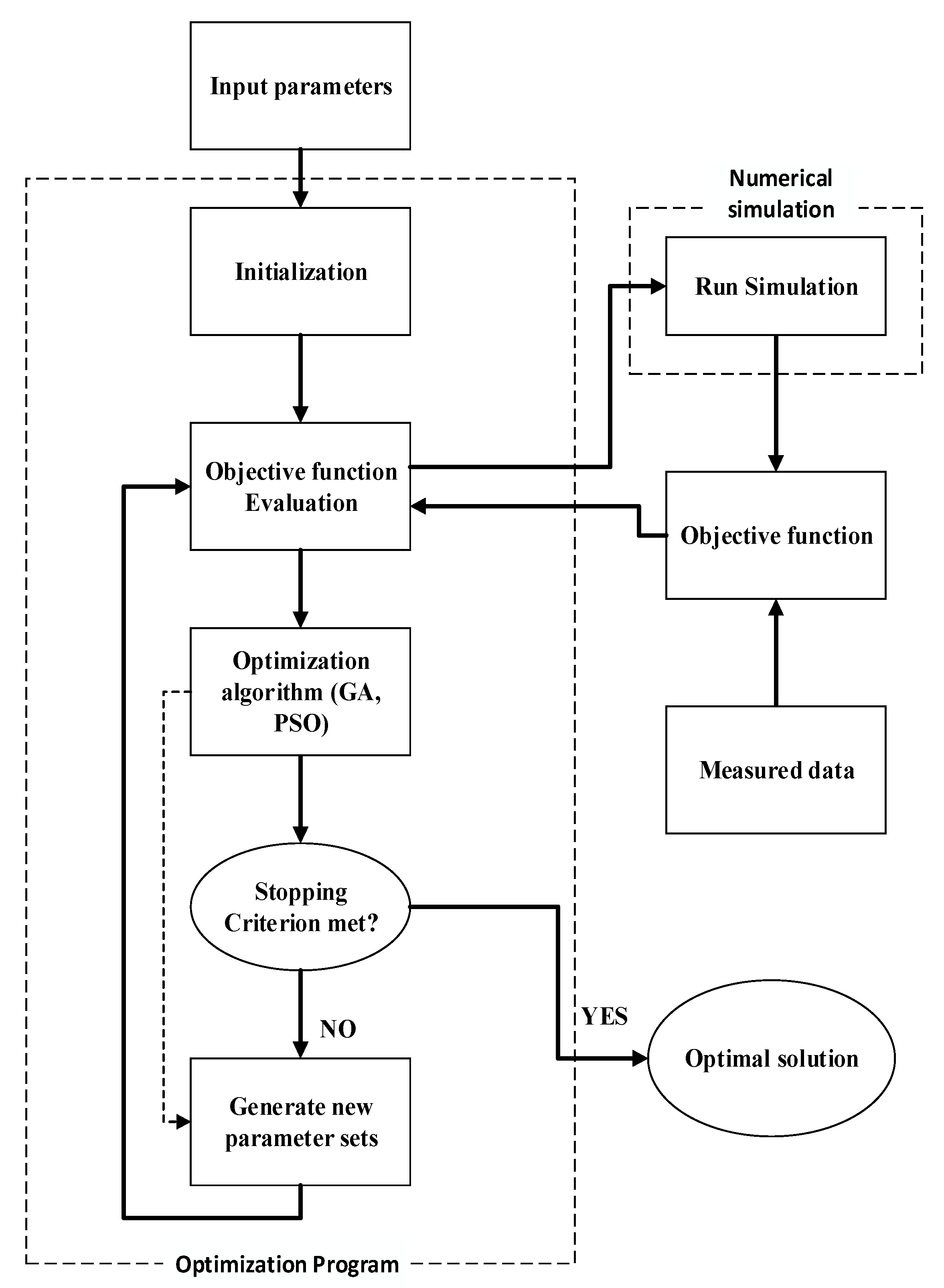
Figure 2.
Optimization strategy for back analysis.
Figure 2.
Optimization strategy for back analysis.
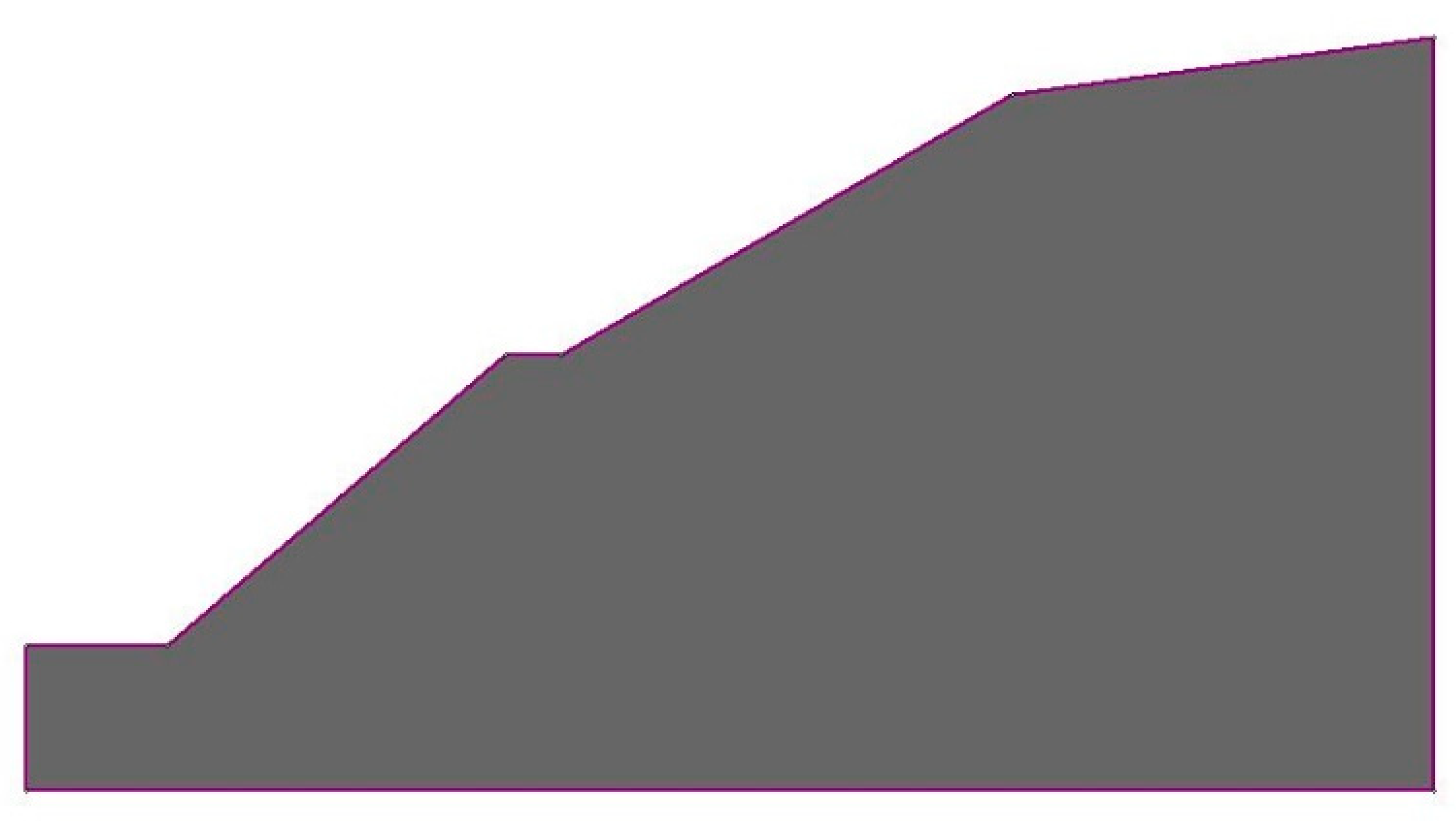
Figure 3.
Model geometry of the slope cross-section.
Figure 3.
Model geometry of the slope cross-section.
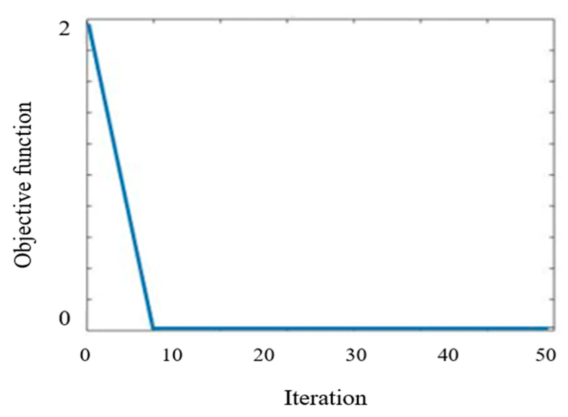
Figure 4.
PSO convergence characteristic for back calculating D.
Figure 4.
PSO convergence characteristic for back calculating D.
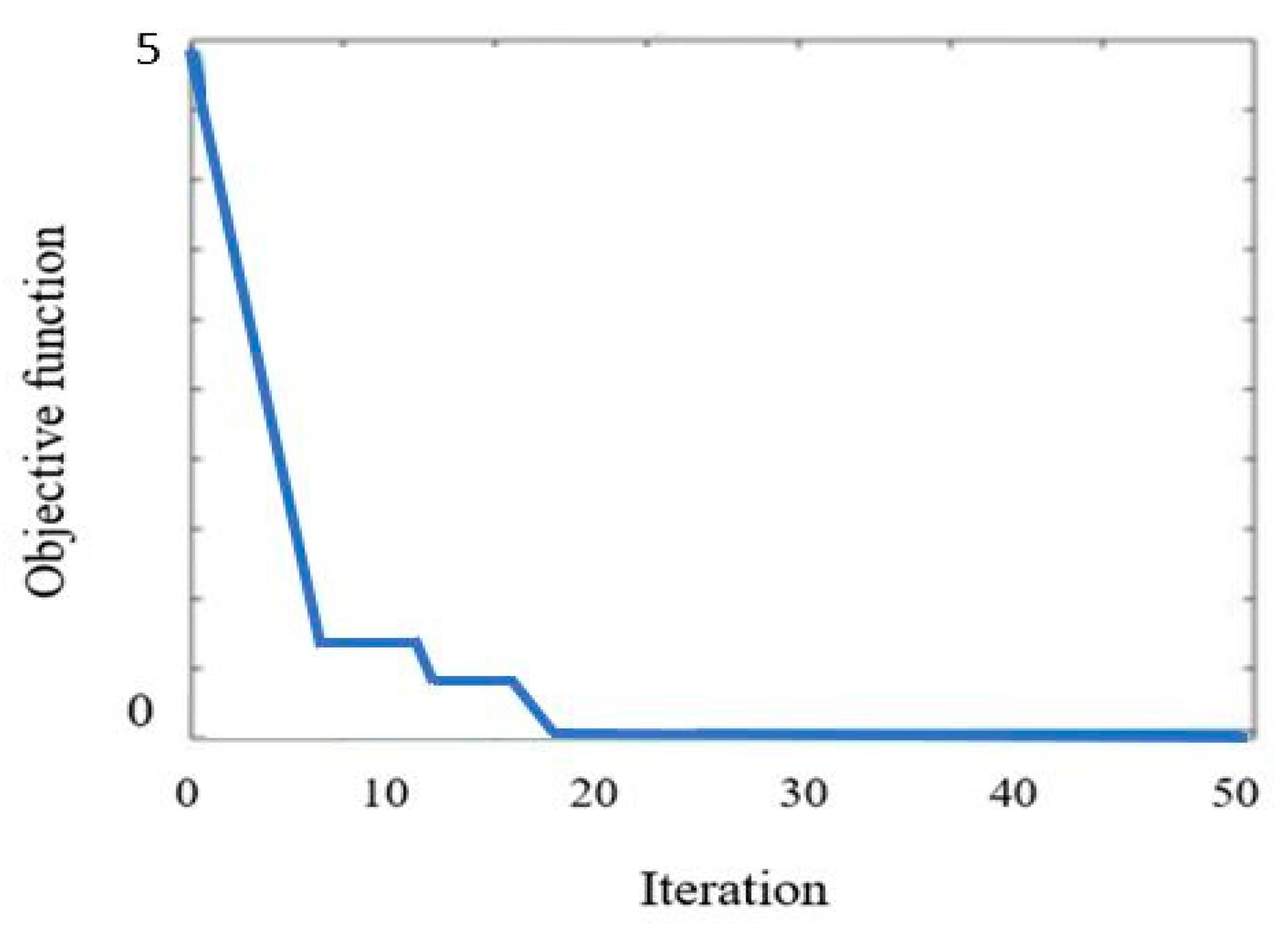
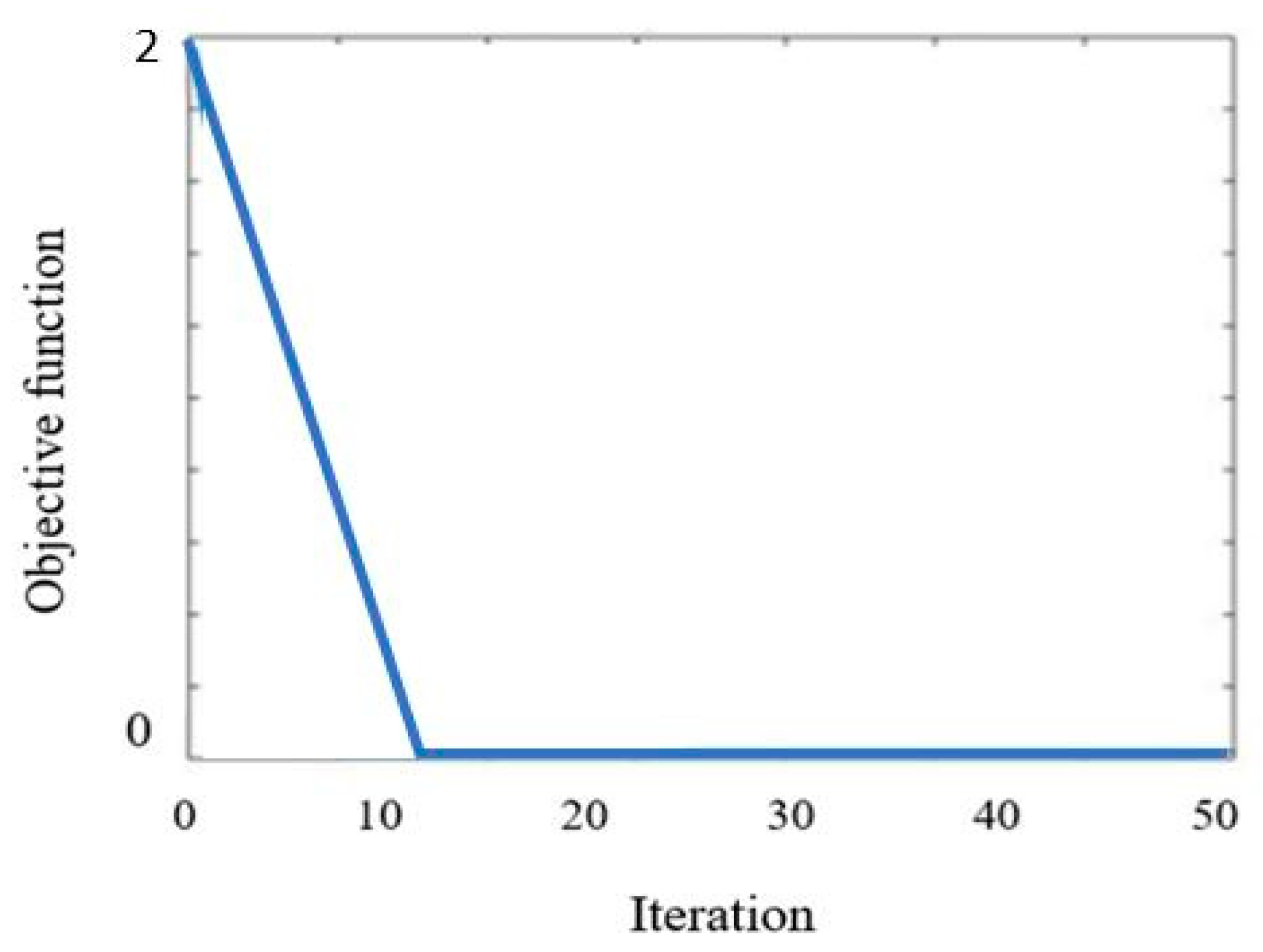
Figure 5.
GA convergence characteristic for back analyzing D.
Figure 5.
GA convergence characteristic for back analyzing D.
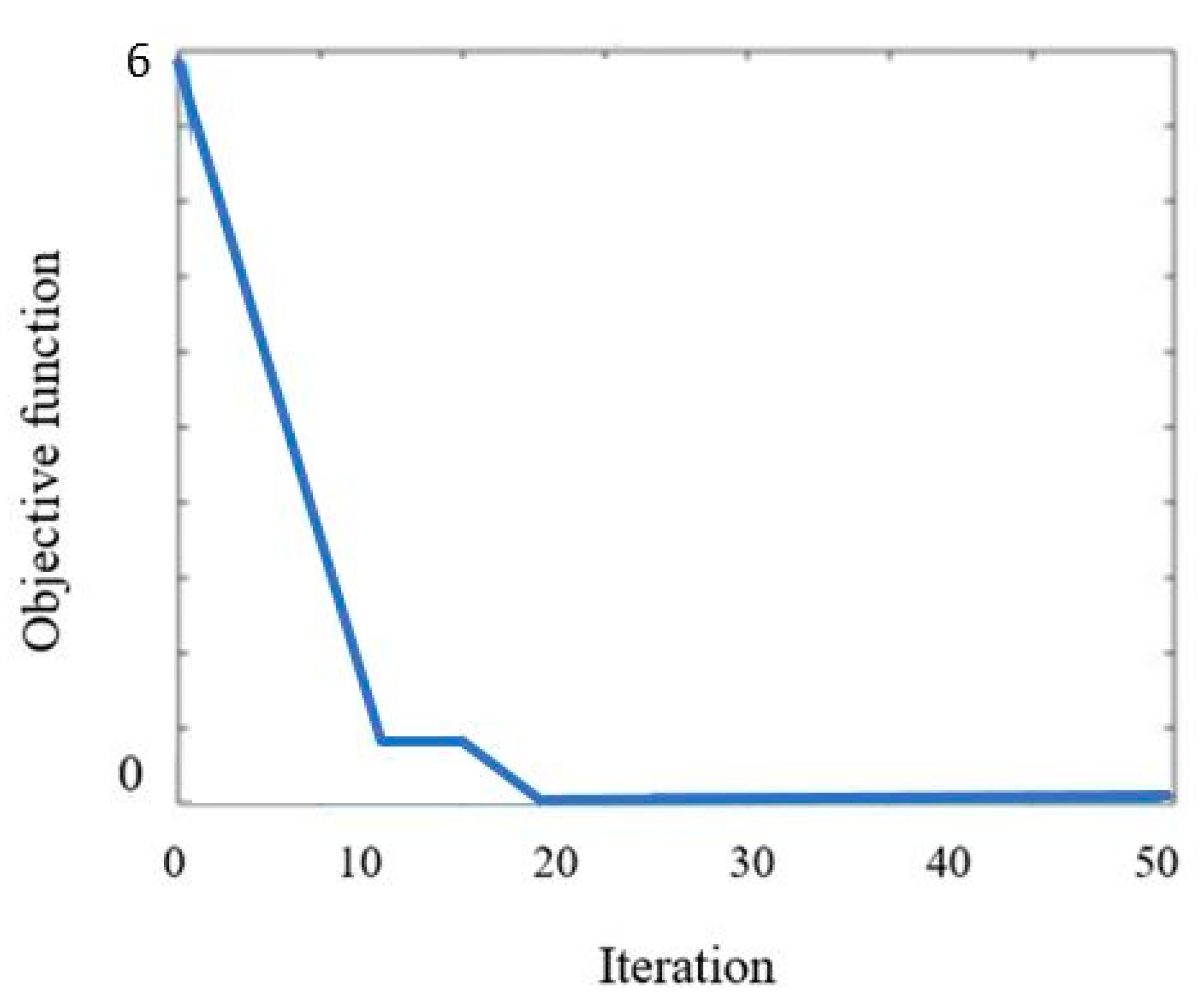
Figure 6.
PSO convergence characteristic for back calculating D, GSI, and .
Figure 6.
PSO convergence characteristic for back calculating D, GSI, and .
Figure 7.
GA convergence characteristic for back calculating D, GSI, and .
Figure 7.
GA convergence characteristic for back calculating D, GSI, and .
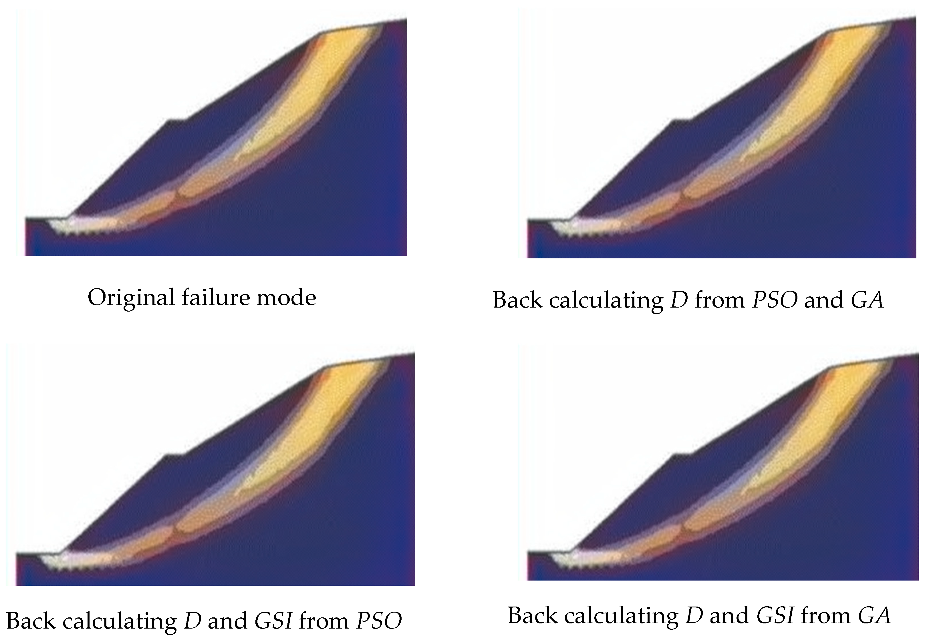
Figure 8.
Comparison of original and back-calculated failure mechanism from PSO and GA.
Figure 8.
Comparison of original and back-calculated failure mechanism from PSO and GA.
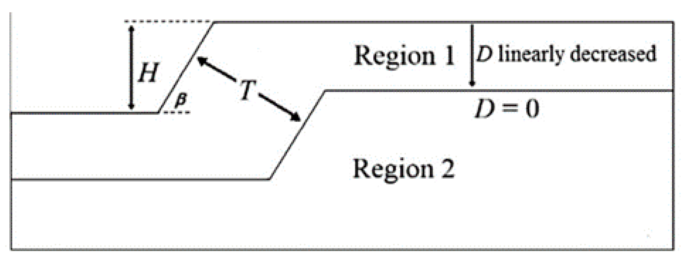
Figure 9.
D linearly decreased with depth in Region 1 of the rock slope.
Figure 9.
D linearly decreased with depth in Region 1 of the rock slope.
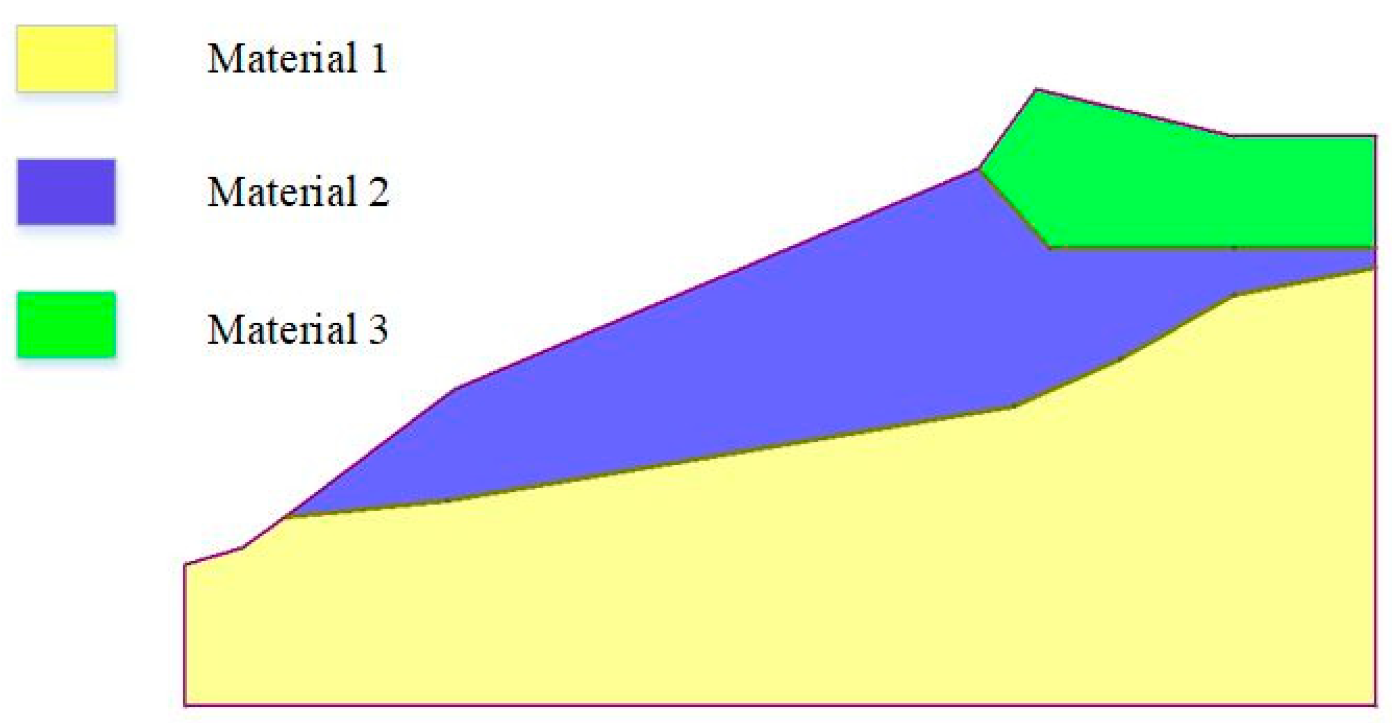
Figure 10.
Model geometry of the slope cross-section.
Figure 10.
Model geometry of the slope cross-section.
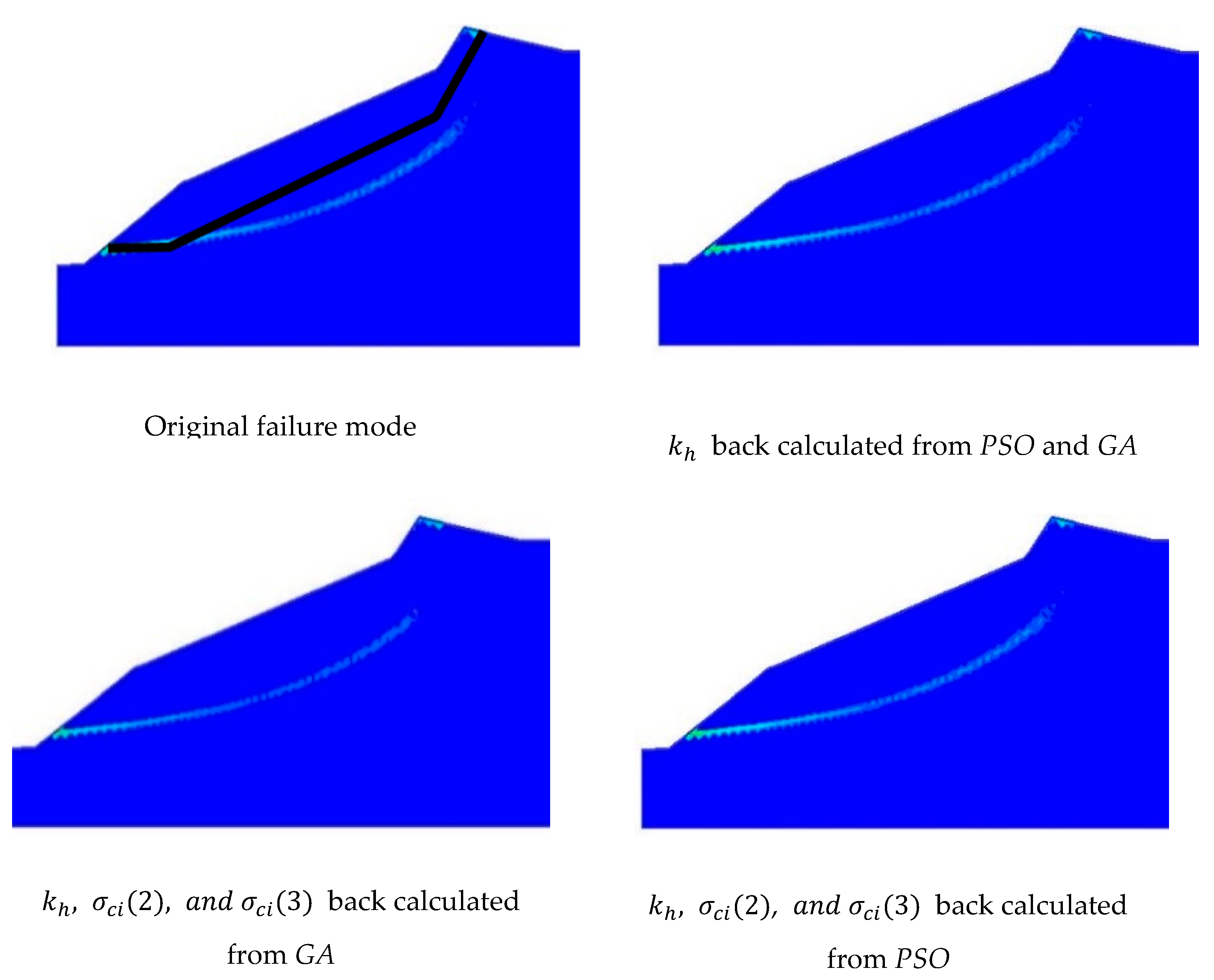
Figure 11.
Comparison of original mode to failure modes of back-calculated parameters with T/H = infinity.
Figure 11.
Comparison of original mode to failure modes of back-calculated parameters with T/H = infinity.
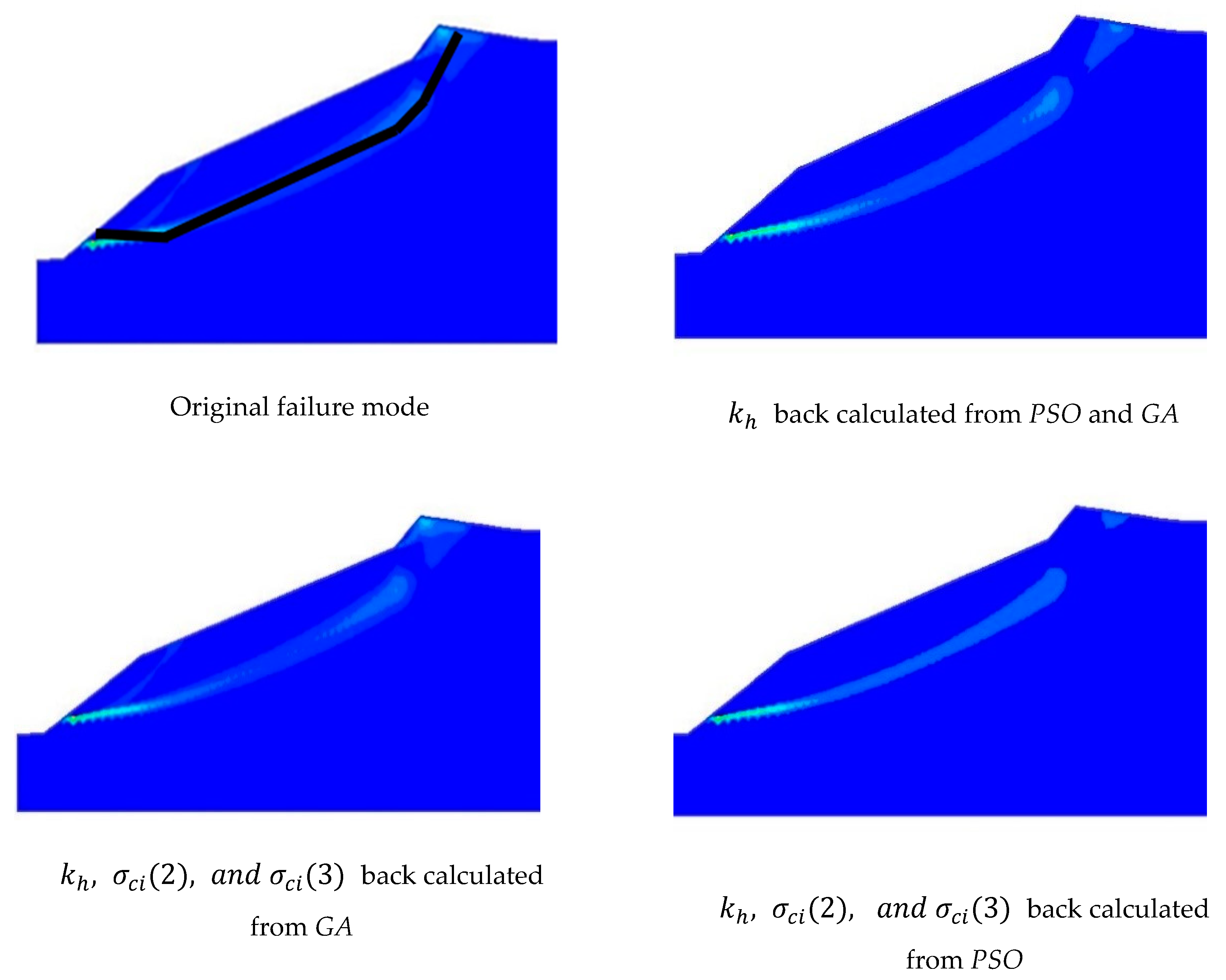
Figure 12.
Comparison of original mode to failure mode of back-calculated parameters with T/H = 2.5.
Figure 12.
Comparison of original mode to failure mode of back-calculated parameters with T/H = 2.5.
Table 1.
Parameters employed in the upper-bound finite element limit analysis (UB-FELA) model.
Table 1.
Parameters employed in the upper-bound finite element limit analysis (UB-FELA) model.
| Parameter | Value |
|---|
| Uniaxial compressive strength () | 5.2 MPa |
| Geological Strength Index (GSI) | 16 |
| Material constant for intact rock mass () | 7 |
Table 2.
Genetic algorithm (GA) parameter setting.
Table 2.
Genetic algorithm (GA) parameter setting.
| Parameter | Value |
|---|
| Population size | 50 |
| Number of generations | 50 |
| Crossover type | Typically two point |
| Crossover rate | 0.6 |
| Mutation types | Bit flip |
| Mutation rate | 0.001 |
Table 3.
Particle swarm optimization (PSO) parameter setting.
Table 3.
Particle swarm optimization (PSO) parameter setting.
| Parameter | Value |
|---|
| Population size | 50 |
| Number of iterations | 50 |
| c1 and c2 | 2 |
| 0.4–0.9 |
| r1 and r2 | 0–1 |
Table 4.
Back-calculated value of disturbance factor (D) from PSO and GA.
Table 4.
Back-calculated value of disturbance factor (D) from PSO and GA.
Table 5.
Back calculated D and GSI from PSO.
Table 5.
Back calculated D and GSI from PSO.
| Parameter | Back-Analyzed Value |
|---|
| D | 0.72 |
| GSI | 17.46 |
Table 6.
Back calculated D and GSI from GA.
Table 6.
Back calculated D and GSI from GA.
| Parameter | Back-Analyzed Value |
|---|
| D | 0.69 |
| GSI | 16.4 |
Table 7.
Back-calculated D, GSI and from PSO.
Table 7.
Back-calculated D, GSI and from PSO.
| Parameter | Back-Analyzed Value |
|---|
| D | 0.51 |
| GSI | 14.2 |
| 5 |
Table 8.
Back-calculated D, GSI and from GA.
Table 8.
Back-calculated D, GSI and from GA.
| Parameter | Back-Analyzed Value |
|---|
| D | 0.62 |
| GSI | 14.41 |
| 6.8 |
Table 9.
Back-calculated D, GSI, and from PSO.
Table 9.
Back-calculated D, GSI, and from PSO.
| Parameter | Back-Analyzed Value |
|---|
| D | 0.77 |
| GSI | 18.00 |
| 8.90 |
| 4.57 MPa |
Table 10.
Back-calculated D, GSI, and from GA.
Table 10.
Back-calculated D, GSI, and from GA.
| Parameter | Back-Analyzed Value |
|---|
| D | 0.59 |
| GSI | 11.00 |
| 8.49 |
| 5.60 MPa |
Table 11.
Standard deviations and ranges for , and .
Table 11.
Standard deviations and ranges for , and .
| Parameter | Mean Value | Standard Deviation (σ) | Range
|
|---|
| GSI | 16 | ±1.6 | 11.2–20.8 |
| 7 | ±0.9 | 4.3–9.7 |
| 5.2 | ±1.3 | 1.3–9.1 |
Table 12.
Mean values of back-calculated parameters from PSO and GA.
Table 12.
Mean values of back-calculated parameters from PSO and GA.
| | PSO | GA |
|---|
| D | GSI | | | D | GSI | | |
|---|
| Scenario A | 0.70 | 17.40 | 7.39 | 5.22 | 0.68 | 16.00 | 6.99 | 5.44 |
| Scenario B | 0.69 | 17.17 | 7.57 | 4.87 | 0.62 | 15.59 | 6.92 | 4.50 |
| Scenario C | 0.71 | 17.25 | 7.27 | 5.38 | 0.69 | 16.04 | 6.89 | 5.69 |
Table 13.
Comparison of coefficients of variation (COVs) from PSO and GA.
Table 13.
Comparison of coefficients of variation (COVs) from PSO and GA.
| | PSO | GA |
|---|
| D | GSI | | | D | GSI | | |
|---|
| Scenario A | 17.98 | 11.79 | 14.50 | 27.55 | 10.23 | 8.62 | 10.59 | 19.93 |
| Scenario B | 14.87 | 11.76 | 13.82 | 26.43 | 9.59 | 8.31 | 9.20 | 19.00 |
| Scenario C | 11.91 | 10.46 | 14.49 | 20.86 | 6.99 | 8.07 | 8.54 | 16.93 |
Table 14.
Input index of the Hoek–Brown experience equations.
Table 14.
Input index of the Hoek–Brown experience equations.
| | | | | |
|---|
| Material 1 | 87.2 | 70 | 7 | 1 |
| Material 2 | 87.2 | 40 | 9 | 1 |
| Material 3 | 43.8 | 40 | 12 | 1 |
Table 15.
Back-calculated values.
Table 15.
Back-calculated values.
| Thickness to Height Ratio (T/H) | GA | PSO |
|---|
| 2.5 | 0.120 | 0.120 |
| Infinity | 0.045 | 0.045 |
Table 16.
Back-calculated and from GA.
Table 16.
Back-calculated and from GA.
| | T/H = Infinity | T/H = 2.5 |
|---|
| | | |
|---|
| Material 2 | 69.22 | 0.011 | 65.64 | 0.07 |
| Material 3 | 43.8 | 0.011 | 41.68 | 0.07 |
Table 17.
Back-calculated and from PSO.
Table 17.
Back-calculated and from PSO.
| | T/H = Infinity | T/H = 2.5 |
|---|
| | | |
|---|
| Material 2 | 68.88 | 0.007 | 67.00 | 0.07 |
| Material 3 | 39.14 | 0.007 | 30.95 | 0.07 |
Table 18.
Back-calculated , and GSI from GA.
Table 18.
Back-calculated , and GSI from GA.
| | T/H = Infinity | T/H = 2.5 |
|---|
| | | | | |
|---|
| Material 2 | 83.2 | 38.46 | 0.008 | 73.56 | 34.75 | 0.019 |
| Material 3 | 32.47 | 38.46 | 0.008 | 35.84 | 34.75 | 0.019 |
Table 19.
Back-calculated , and GSI from PSO.
Table 19.
Back-calculated , and GSI from PSO.
| | T/H = Infinity | T/H = 2.5 |
|---|
| | | | | |
|---|
| Material 2 | 78.77 | 38.79 | 0.010 | 86.1 | 33.59 | 0.010 |
| Material 3 | 39.56 | 38.79 | 0.010 | 37.63 | 33.59 | 0.010 |
Table 20.
Back-calculated , , GSI and from GA.
Table 20.
Back-calculated , , GSI and from GA.
| | T/H = Infinity | T/H = 2.5 |
|---|
| | | | | | | |
|---|
| Material 2 | 80.47 | 8.72 | 39.82 | 0.015 | 77.94 | 7.29 | 38.73 | 0.043 |
| Material 3 | 38.28 | 8.02 | 39.82 | 0.015 | 34.43 | 11.27 | 38.73 | 0.043 |
Table 21.
Back-calculated , , GSI and from PSO.
Table 21.
Back-calculated , , GSI and from PSO.
| | T/H = Infinity | T/H = 2.5 |
|---|
| | | | | | | |
|---|
| Material 2 | 89.54 | 8.45 | 39.94 | 0.013 | 77.64 | 7.66 | 36.11 | 0.02 |
| Material 3 | 35.43 | 8.97 | 39.94 | 0.013 | 43.21 | 11.97 | 36.11 | 0.02 |
Table 22.
Range of parameters for back calculation.
Table 22.
Range of parameters for back calculation.
| | | | | |
|---|
| Material 2 | 44–130 | 6.7–11.3 | 32–48 | 0–1 |
| Material 3 | 22–66 | 9–15 | 32–48 | 0–1 |
Table 23.
Mean value of back-calculated parameters for T/H = 2.5.
Table 23.
Mean value of back-calculated parameters for T/H = 2.5.
| | GA | PSO |
|---|
| | | | | | | |
|---|
| Material 2 | 84.65 | 9.23 | 41.87 | 0.012 | 85.48 | 8.81 | 43.24 | 0.14 |
| Material 3 | 44.51 | 11.74 | 41.87 | 0.012 | 52.08 | 11.65 | 43.24 | 0.14 |
Table 24.
Mean values of back-calculated parameters for T/H = infinity.
Table 24.
Mean values of back-calculated parameters for T/H = infinity.
| | GA | PSO |
|---|
| | | | | | | |
|---|
| Material 2 | 99.60 | 11.37 | 42.28 | 0.11 | 92.27 | 9.05 | 42.52 | 0.09 |
| Material 3 | 46.84 | 11.33 | 42.28 | 0.11 | 50.52 | 12.63 | 42.52 | 0.09 |
Table 25.
COVs of back-calculated parameters for T/H = 2.5.
Table 25.
COVs of back-calculated parameters for T/H = 2.5.
| | GA | PSO |
|---|
| | | | | | | |
|---|
| Material 2 | 27.46 | 13.29 | 7.83 | 39.75 | 18.68 | 9.94 | 6.84 | 44.98 |
| Material 3 | 18.38 | 9.47 | 7.83 | 39.75 | 23.14 | 14.39 | 6.84 | 44.98 |
Table 26.
COVs of back-calculated parameters for T/H = infinity.
Table 26.
COVs of back-calculated parameters for T/H = infinity.
| | GA | PSO |
|---|
| | | | | | | |
|---|
| Material 2 | 11.12 | 11.37 | 6.95 | 43.49 | 19.93 | 11.80 | 6.20 | 44.94 |
| Material 3 | 17.89 | 11.33 | 6.95 | 43.49 | 13.57 | 12.41 | 6.20 | 44.94 |


