A Novel Fuzzy Linear Regression Sliding Window GARCH Model for Time-Series Forecasting

 , ,
, , 
Abstract
1. Introduction
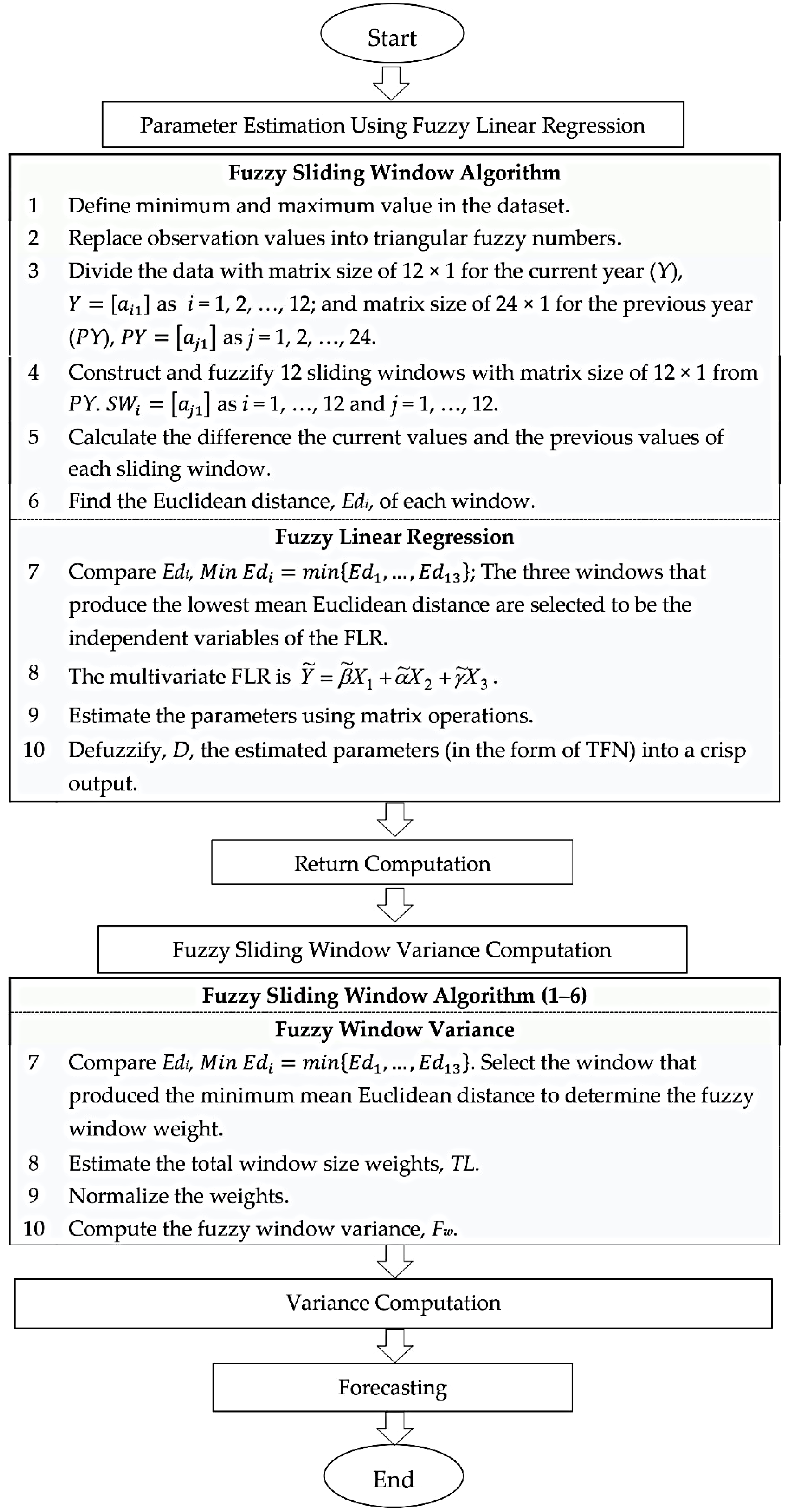
2. The Proposed Model
2.1. FLR-FSWGARCH Model
2.1.1. Parameter Estimation Using Fuzzy Linear Regression
2.1.2. Return Computation
2.1.3. Fuzzy Window Variance Computation
2.1.4. Forecasting
2.2. Validation and Evaluation of the Proposed Model
3. Implementations and Results
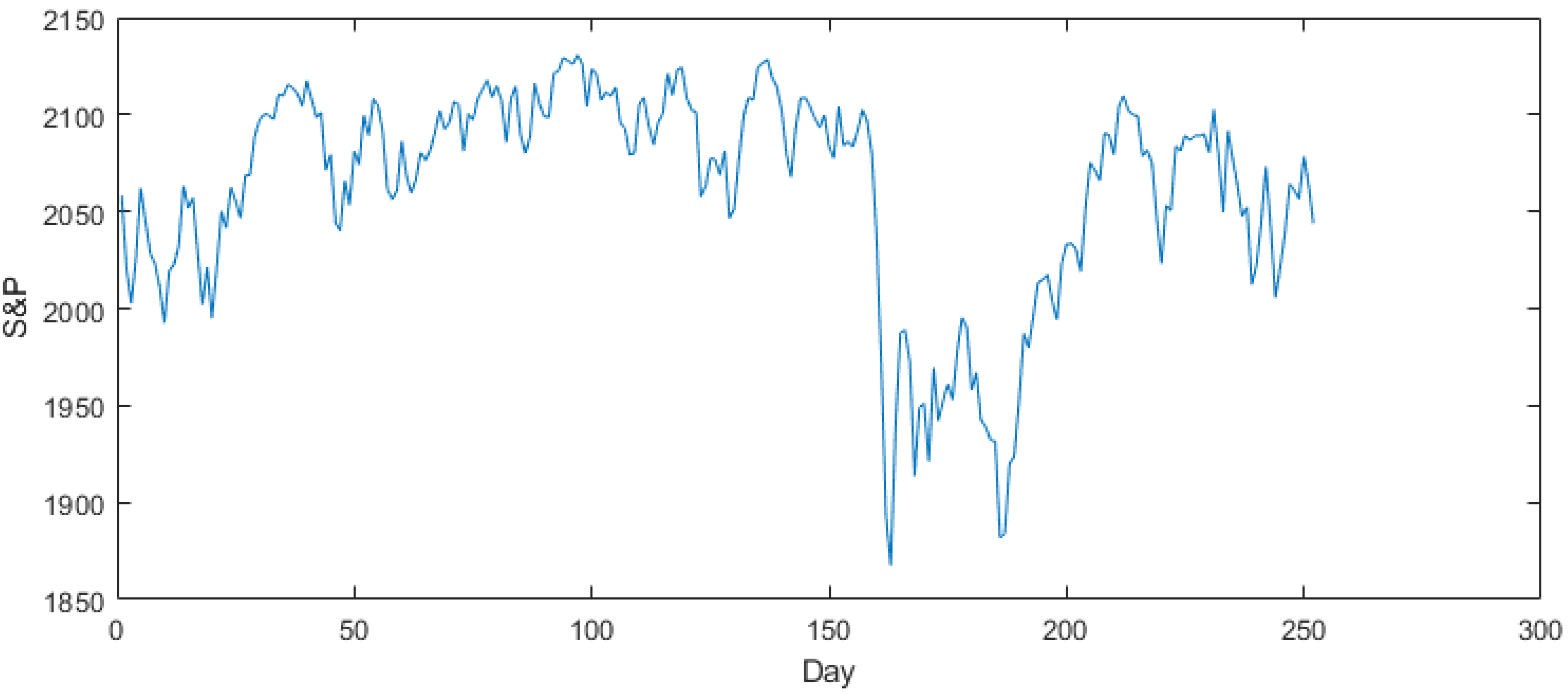
3.1. Forecasting of the Stock and Price (S&P) Index Using the FLR-FSWGARCH Model
- The difference between the current and previous values (only displays the calculation of the first row).
- The defuzzification:
- The mean Euclidean distance:The Euclidean distance calculated for each sliding window is shown in Table 2.
3.2. Comparison and Evaluation of the Proposed FLR-FSWGARCH Model with Benchmark Models for Two Datasets
4. Conclusions
Author Contributions
Funding
Acknowledgments
Conflicts of Interest
References
- Tobar, F.A.; Orchard, M.E.; Mandic, D.P.; Constantinides, A.G. Estimation of Financial Indices Volatility Using a Model with Time-Varying Parameters. In Proceedings of the IEEE Conference on Computational Intelligence for Financial Engineering & Economics (CIFEr), London, UK, 27–28 March 2014; pp. 318–324. [Google Scholar] [CrossRef]
- Banik, S.; Khan, K. Forecasting US NASDAQ Stock Index Values Using Hybrid Forecasting Systems. In Proceedings of the 18th International Conference on Computer and Information Technology (ICCIT), Dhaka, Bangladesh, 21–23 December 2015; pp. 282–287. [Google Scholar] [CrossRef]
- Zou, Y.; Donner, R.V.; Marwan, N.; Donges, J.F.; Kurths, J. Complex Network Approaches to Nonlinear Time Series Analysis. Phys. Rep. 2019, 787, 1–97. [Google Scholar] [CrossRef]
- Ruekkasaem, L.; Sasananan, M. Forecasting Agricultural Products Prices Using Time Series Methods for Crop Planning. Int. J. Mech. Eng. Technol. (Ijmet) 2018, 9, 957–971. [Google Scholar]
- Dong, M.A. Tutorial on Nonlinear Time-Series Data Mining in Engineering Asset Health and Reliability Prediction: Concepts, Models, and Algorithms. Math. Probl. Eng. 2010, 1–22. [Google Scholar] [CrossRef]
- Bollerslev, T. Generalized Autoregressive Conditional Heteroskedasticity. J. Econom. 1986, 31, 307–327. [Google Scholar] [CrossRef]
- Lamoureux, C.G.; Lastrapes, W.D. Persistence in Variance, Structural Change, and the GARCH Model. J. Bus. Econ. Stat. 1990, 8, 225–234. [Google Scholar] [CrossRef]
- Mosalaosi, M.; Afullo, T.J.O. Prediction of Asynchronous Impulsive Noise Volatility for Indoor Powerline Communication Systems Using GARCH Models. In Proceedings of the Progress in Electromagnetic Research Symposium (PIERS), Shanghai, China, 8–11 August 2016; pp. 4876–4880. [Google Scholar] [CrossRef]
- Guo, H. Estimating Volatilities by The GARCH and The EWMA Model of Petrochina and TCL in The Stock Exchange Market of China. In Proceedings of the 6th International Scientific Conference Managing and Modelling of Financial Risks, Ostrava, Czech Republic, 10–11 September 2012; pp. 191–202. [Google Scholar]
- Naimy, V.Y.; Hayek, M.R. Modelling and Predicting the Bitcoin Volatility Using GARCH Models. Int. J. Math. Model. Numer. Optim. 2018, 8, 197. [Google Scholar] [CrossRef]
- Glosten, L.R.; Jagannathan, R.; Runkle, D.E. On the Relation between the Expected Value and the Volatility of the Nominal Excess Return on Stocks. J. Financ. 1993, 48, 1779–1801. [Google Scholar] [CrossRef]
- Ma, X.; Yang, R.; Zou, D.; Liu, R. Measuring Extreme Risk of Sustainable Financial System Using GJR-GARCH Model Trading Data-Based. Int. J. Inf. Manag. 2020, 50, 526–537. [Google Scholar] [CrossRef]
- Donaldson, R.G.; Kamstra, M. An Artificial Neural Network-GARCH Model for International Stock Return Volatility. J. Empir. Financ. 1997, 4, 17–46. [Google Scholar] [CrossRef]
- Lu, X.; Que, D.; Cao, G. Volatility Forecast Based on the Hybrid Artificial Neural Network and GARCH-Type Models. Procedia Comput. Sci. 2016, 91, 1044–1049. [Google Scholar] [CrossRef]
- Van der Weide, R. GO-GARCH: A Multivariate Generalized Orthogonal GARCH Model. J. Appl. Econom. 2002, 17, 549–564. [Google Scholar] [CrossRef]
- Jondeau, E.; Rockinger, M. The Copula-GARCH Model of Conditional Dependencies: An International Stock Market Application. J. Int. Money Financ. 2006, 25, 827–853. [Google Scholar] [CrossRef]
- Bollerslev, T.; Patton, A.J.; Quaedvlieg, R. Multivariate Leverage Effects and Realized Semi-covariance GARCH Models. J. Econom. 2020. [Google Scholar] [CrossRef]
- Engle, R.F.; Rangel, J.G. The Spline-GARCH Model for Low-Frequency Volatility and Its Global Macroeconomic Causes. Rev. Financ. Stud. 2008, 21, 1187–1222. [Google Scholar] [CrossRef]
- Babu, C.N.; Reddy, B.E. Selected Indian Stock Predictions Using a Hybrid ARIMA-GARCH Model. In Proceedings of the International Conference on Advances in Electronics Computers and Communications, Bangalore, India, 10–11 October 2014; pp. 1–6. [Google Scholar] [CrossRef]
- Ou, P.; Wang, H. Modeling and Forecasting Stock Market Volatility by Gaussian Processes based on GARCH, EGARCH and GJR Models. In Proceedings of the World Congress on Engineering, London, UK, 6–8 July 2011; pp. 338–342. [Google Scholar]
- Choudhry, T.; Hasan, M.; Zhang, Y. Forecasting the Daily Dynamic Hedge Ratios in Emerging European Stock Futures Markets: Evidence from GARCH Models. Int. J. Bank. Account. Financ. 2019, 10, 67–100. [Google Scholar] [CrossRef]
- Maciel, L. A Hybrid Fuzzy GJR-GARCH Modeling Approach for Stock Market Volatility Forecasting. Braz. Rev. Financ. 2012, 10, 337–367. [Google Scholar] [CrossRef]
- Wang, Y.H. Nonlinear Neural Network Forecasting Model for Stock Index Option Price: Hybrid GJR–GARCH Approach. Expert Syst. Appl. 2009, 36, 564–570. [Google Scholar] [CrossRef]
- Kristjanpoller, W.; Fadic, A.; Minutolo, M.C. Volatility Forecast Using Hybrid Neural Network Models. Expert Syst. Appl. 2014, 41, 2437–2442. [Google Scholar] [CrossRef]
- Mao, H.; Zhu, F.; Cui, Y. A Generalized Mixture Integer-Valued GARCH Model. Stat. Methods Appl. 2019, 1–26. [Google Scholar] [CrossRef]
- Lin, Y.; Xiao, Y.; Li, F. Forecasting Crude Oil Price Volatility Via A HM-EGARCH Model. Energy Econ. 2020, 104693. [Google Scholar] [CrossRef]
- Shbier, M.Z.; Ku-Mahamud, K.R.; Othman, M. SWGARCH Model for Time Series Forecasting. In Proceedings of the 1st International Conference on Internet of Things and Machine Learning, Liverpool, UK, 17–18 October 2017. [Google Scholar] [CrossRef]
- Hanapi, A.L.M.; Othman, M.; Sokkalingam, R.; Sakidin, H. Developed A Hybrid Sliding Window and GARCH Model for Forecasting of Crude Palm Oil Prices in Malaysia. J. Phys. Conf. Ser. 2018, 1123, 1–8. [Google Scholar] [CrossRef]
- Kapoor, P.; Bedi, S.S. Weather Forecasting Using Sliding Window Algorithm. ISRN Signal Process. 2013, 1–5. [Google Scholar] [CrossRef]
- Tealab, A.; Hefny, H.; Badr, A. Forecasting of Nonlinear Time Series Using ANN. Future Comput. Inform. J. 2017, 2, 39–47. [Google Scholar] [CrossRef]
- Singh, P.; Gaurav, D. A Hybrid Fuzzy Time Series Forecasting Model Based on Granular Computing and Bio-Inspired Optimization Approaches. J. Comput. Sci. 2018, 27, 370–385. [Google Scholar] [CrossRef]
- Mas-Machuca, M.; Sainz, M.; Martinez-Costa, C. A Review of Forecasting Models for New Products. Intang. Cap. 2017, 10, 1–25. [Google Scholar] [CrossRef][Green Version]
- Dincer, N.G.; Akkuş, Ö. A New Fuzzy Time Series Model Based on Robust Clustering for Forecasting of Air Pollution. Ecol. Inform. 2018, 43, 157–164. [Google Scholar] [CrossRef]
- Chang, J.-R.; Wei, L.-Y.; Cheng, C.H. A Hybrid ANFIS Model Based on AR and Volatility for TAIEX Forecasting. Appl. Soft Comput. 2011, 11, 1388–1395. [Google Scholar] [CrossRef]
- Korkmaz, T.; Aydın, K. Using EVMA and GARCH Methods in VaR Calculations: Aplication on ISE-30 Index. Available online: http://content.csbs.utah.edu/~ehrbar/erc2002/pdf/P161.pdf (accessed on 12 March 2020).
- Abdullah, L.; Zakaria, N. Matrix Driven Multivariate Fuzzy Linear Regression Model in Car Sales. J. Appl. Sci. 2012, 12, 56–63. [Google Scholar] [CrossRef]
- Jialu, X.; Qiujun, L.G. Outlier Detection in Fuzzy Linear Regression About Predicting GDP. Int. J. Recent Res. Appl. Stud. 2014, 19, 189–193. [Google Scholar]
- Muzzioli, S.; Ruggier, A.; De Baets, B. A Comparison of Fuzzy Regression Methods for The Estimation of the Implied Volatility Smile Function. Fuzzy Sets Syst. 2015, 266, 131–143. [Google Scholar] [CrossRef]
- Bingham, E.; Gionis, A.; Haiminen, N.; Hiisila, H.; Mannila, H.; Terzi, E. Segmentation and Dimensionality Reduction. In Proceedings of the Sixth SIAM International Conference on Data Mining, Bethesda, MD, USA, 20–22 April 2006; pp. 372–383. [Google Scholar] [CrossRef]
- Datar, M.; Gionis, A.; Indyk, P.; Motwani, R. Maintaining Stream Statistics Over Sliding Windows. In Proceedings of the Thirteenth Annual ACM-SIAM Symposium on Discrete Algorithms, San Francisco, CA, USA, 6–8 January 2002; pp. 1794–1813. [Google Scholar] [CrossRef]
- Ferreira, P.; Dionísio, A.; Guedes, E.F.; Zebendee, G.F. A Sliding Windows Approach to Analyse the Evolution of Bank Shares in The European Union. Phys. A Stat. Mech. Its Appl. 2018, 490, 1355–1367. [Google Scholar] [CrossRef]
- Kapila, T.R.R.; Seneviratna, M.D.; Jianguo, W.; Arumawadu, H.I. A Hybrid Statistical Approach for Stock Market Forecasting Based on Artificial Neural Network and ARIMA Time Series Models. In Proceedings of the International Conference on Behavioral, Economic and Socio-cultural Computing (BESC), Nanjing, China, 30 October–1 November 2015; pp. 54–60. [Google Scholar] [CrossRef]


| Sliding Window, SWi | Mean of Edi |
|---|---|
| 1 | 111.8034 |
| 2 | 141.4214 |
| 3 | 132.2876 |
| 4 | 111.8034 |
| 5 | 111.8034 |
| 6 | 141.4214 |
| 7 | 150.0000 |
| 8 | 141.4214 |
| 9 | 158.1139 |
| 10 | 193.6492 |
| 11 | 187.0829 |
| 12 | 180.2776 |
| Day | S&P | Return | Fuzzy Window Variance | Variance |
|---|---|---|---|---|
| 1 | 2058.20 | |||
| 2 | 2020.58 | 3.40 × 10⁻⁴ | ||
| 3 | 2002.61 | 7.98 × 10⁻⁵ | ||
| 4 | 2025.90 | 1.34 × 10⁻⁴ | ||
| 5 | 2062.14 | 3.14 × 10⁻⁴ | ||
| 6 | 2044.81 | 7.12 × 10⁻⁵ | 1.67636 × 10⁻⁴ | 1.6764 × 10⁻⁴ |
| 7 | 2028.26 | 6.60 × 10⁻⁵ | 1.27025 × 10⁻⁴ | 1.3585 × 10⁻⁴ |
| 8 | 2023.03 | 6.67 × 10⁻⁶ | 8.49053 × 10⁻⁵ | 1.0901 × 10⁻⁴ |
| 9 | 2011.27 | 3.40 × 10⁻⁵ | 5.67693 × 10⁻⁵ | 7.3588 × 10⁻⁵ |
| 10 | 1992.67 | 8.63 × 10⁻⁵ | 5.27244 × 10⁻⁵ | 5.9790 × 10⁻⁵ |
| ⋮ | ⋮ | ⋮ | ⋮ | ⋮ |
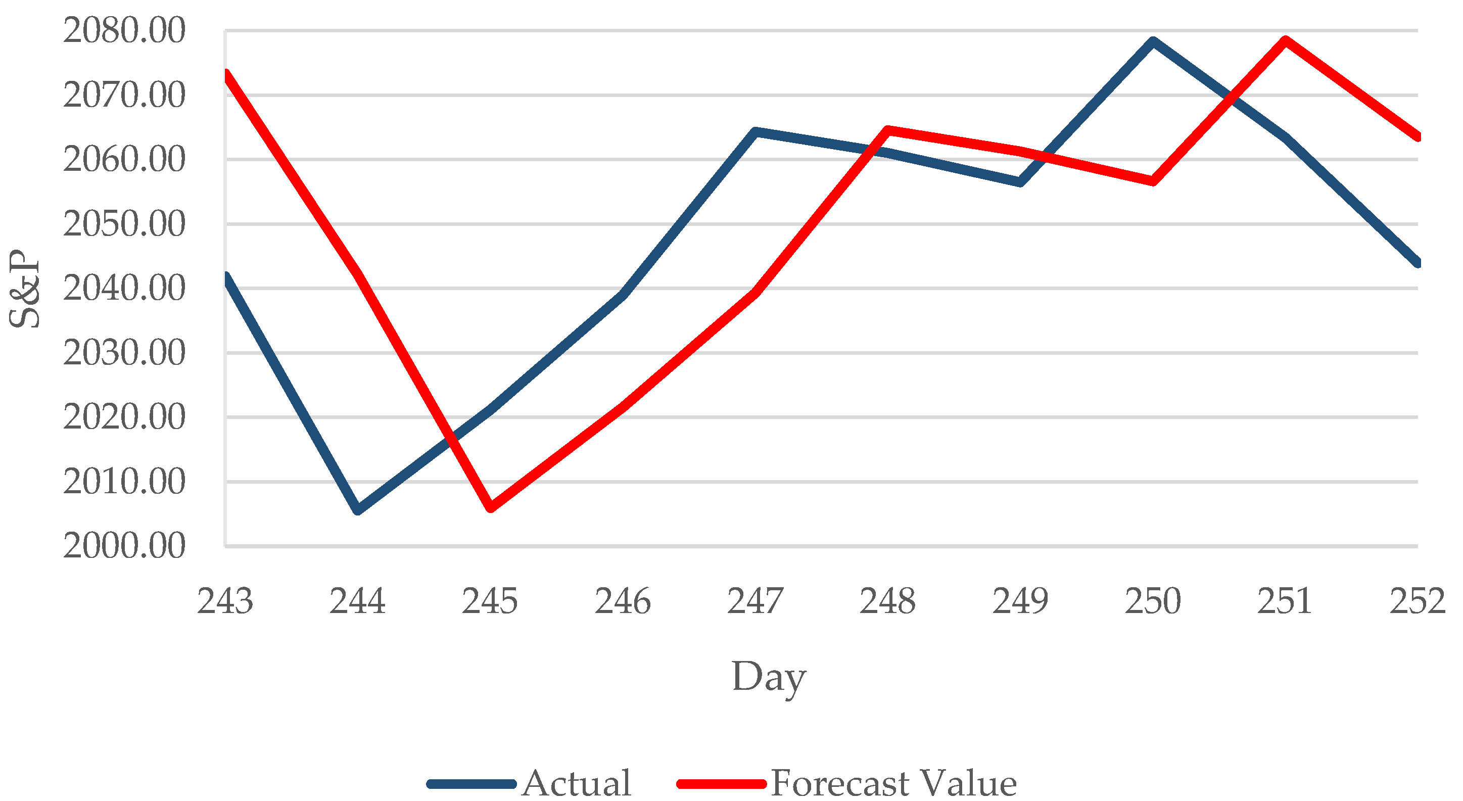
| Day | S&P | Forecast Value | |Percentage Error| |
|---|---|---|---|
| 243 | 2041.89 | 2073.34 | 1.5403 |
| 244 | 2005.55 | 2042.22 | 1.8284 |
| 245 | 2021.15 | 2005.94 | 0.7526 |
| 246 | 2038.97 | 2021.58 | 0.8528 |
| 247 | 2064.29 | 2039.30 | 1.2104 |
| 248 | 2060.99 | 2064.58 | 0.1741 |
| 249 | 2056.50 | 2061.25 | 0.2309 |
| 250 | 2078.36 | 2056.66 | 1.0440 |
| 251 | 2063.36 | 2078.49 | 0.7332 |
| 252 | 2043.94 | 2063.51 | 0.9573 |
| Error | MAPE | ||
|---|---|---|---|
| Model | S&P Dataset | Vanilla Production Dataset | |
| FLR-FSWGARCH | 0.69687 | 11.5308 | |
| SWGARCH | 0.70105 | 26.6458 | |
| GARCH | 0.71922 | 25.6947 | |
| ARIMA-GARCH | 0.70728 | 20.8743 | |
| EWMA | 0.69720 | 26.8468 | |
| Regression Statistics | |||||
| Multiple R | 0.9981 | ||||
| R2 | 0.9962 | ||||
| Adjusted R2 | 0.9962 | ||||
| Standard Error | 6.449 × 10⁻⁶ | ||||
| Observations | 245 | ||||
| df | SS | MS | F | Significance F | |
| Regression | 3 | 2.632 × 10⁻⁶ | 8.773 × 10⁻⁷ | 2.109 × 10⁴ | 2.404 × 10−291 |
| Residual | 241 | 1.003 × 10⁻⁸ | 4.160 × 10⁻¹¹ | ||
| Total | 244 | 2.642 × 10⁻⁶ | |||
| Coefficients | Standard Error | t Statistic | p-Value | ||
| Intercept | 1.912 × 10⁻⁷ | 5.797 × 10⁻⁷ | 0.3299 | 0.7418 | |
| Fw | 0.08091 | 7.631 × 10⁻³ | 10.60 | 8.244 × 10⁻²² | |
| 0.1257 | 2.609 × 10⁻³ | 48.20 | 9.879 × 10−126 | ||
| 0.7909 | 9.013 × 10⁻³ | 87.75 | 6.560 × 10−185 | ||
| Regression Statistics | |||||
| Multiple R | 0.9999 | ||||
| R2 | 0.9999 | ||||
| Adjusted R2 | 0.9999 | ||||
| Standard Error | 8.443 × 10⁻⁴ | ||||
| Observations | 46 | ||||
| df | SS | MS | F | Significance F | |
| Regression | 3 | 1.690 | 0.5634 | 7.894 × 10⁵ | 8.844 × 10−100 |
| Residual | 42 | 2.998 × 10⁻⁵ | 7.137 × 10⁻⁷ | ||
| Total | 45 | 1.690 | |||
| Coefficients | Standard Error | t Statistic | p-Value | ||
| Intercept | 1.921 × 10⁻⁴ | 1.573 × 10⁻⁴ | 1.221 | 0.2290 | |
| Fw | 0.6349 | 4.979 × 10⁻⁴ | 1275 | 5.517 × 10−98 | |
| 0.3013 | 1.099 × 10⁻³ | 274.0 | 6.088 × 10−70 | ||
| 0.06328 | 1.447 × 10⁻³ | 43.72 | 1.184 × 10−36 | ||
© 2020 by the authors. Licensee MDPI, Basel, Switzerland. This article is an open access article distributed under the terms and conditions of the Creative Commons Attribution (CC BY) license (http://creativecommons.org/licenses/by/4.0/).
Share and Cite
Mohamad Hanapi, A.L.; Othman, M.; Sokkalingam, R.; Ramli, N.; Husin, A.; Vasant, P. A Novel Fuzzy Linear Regression Sliding Window GARCH Model for Time-Series Forecasting. Appl. Sci. 2020, 10, 1949. https://doi.org/10.3390/app10061949
Mohamad Hanapi AL, Othman M, Sokkalingam R, Ramli N, Husin A, Vasant P. A Novel Fuzzy Linear Regression Sliding Window GARCH Model for Time-Series Forecasting. Applied Sciences. 2020; 10(6):1949. https://doi.org/10.3390/app10061949
Chicago/Turabian StyleMohamad Hanapi, Amiratul L., Mahmod Othman, Rajalingam Sokkalingam, Nazirah Ramli, Abdullah Husin, and Pandian Vasant. 2020. "A Novel Fuzzy Linear Regression Sliding Window GARCH Model for Time-Series Forecasting" Applied Sciences 10, no. 6: 1949. https://doi.org/10.3390/app10061949
APA StyleMohamad Hanapi, A. L., Othman, M., Sokkalingam, R., Ramli, N., Husin, A., & Vasant, P. (2020). A Novel Fuzzy Linear Regression Sliding Window GARCH Model for Time-Series Forecasting. Applied Sciences, 10(6), 1949. https://doi.org/10.3390/app10061949