Dynamics Modeling and Theoretical Study of the Two-Axis Four-Gimbal Coarse–Fine Composite UAV Electro-Optical Pod


Abstract
1. Introduction
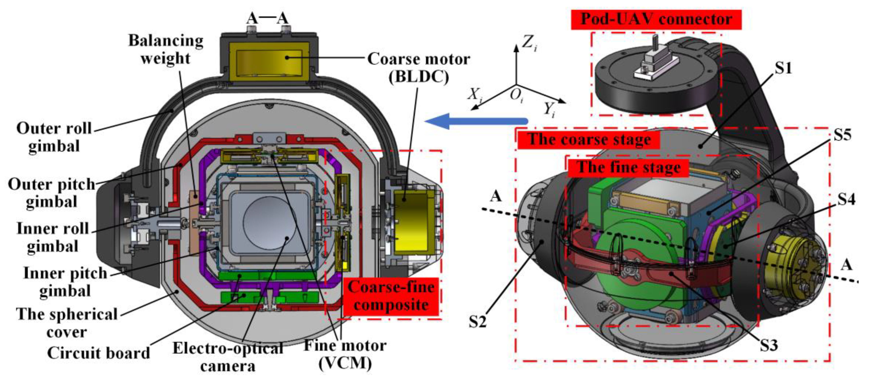
2. Structure Design
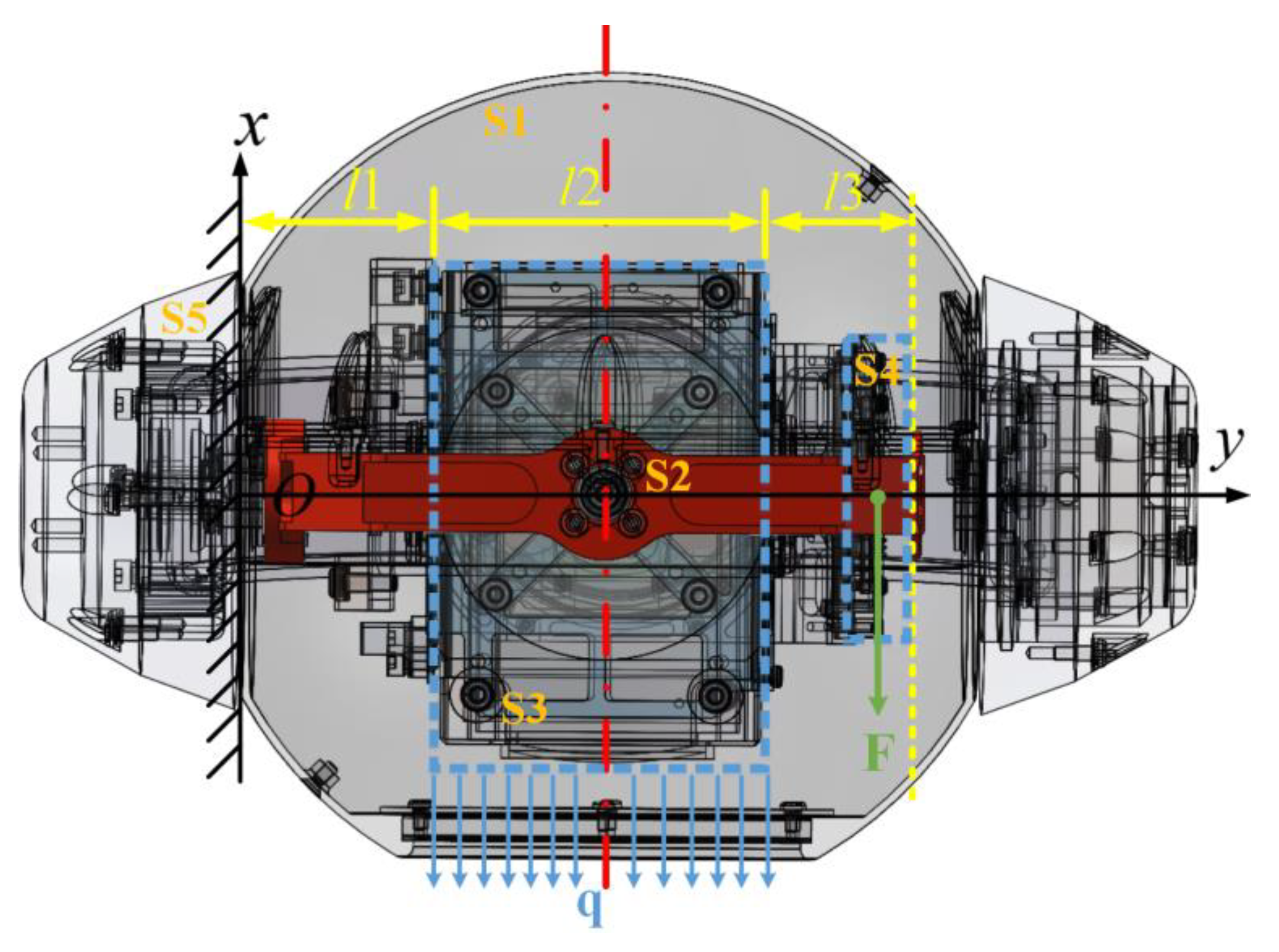
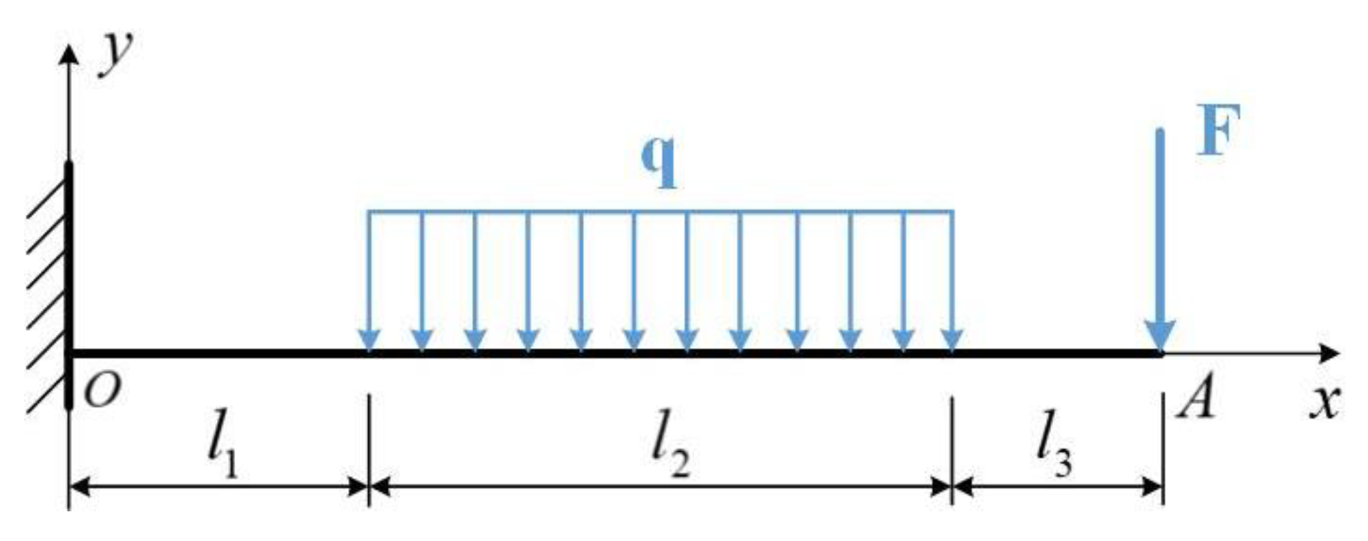
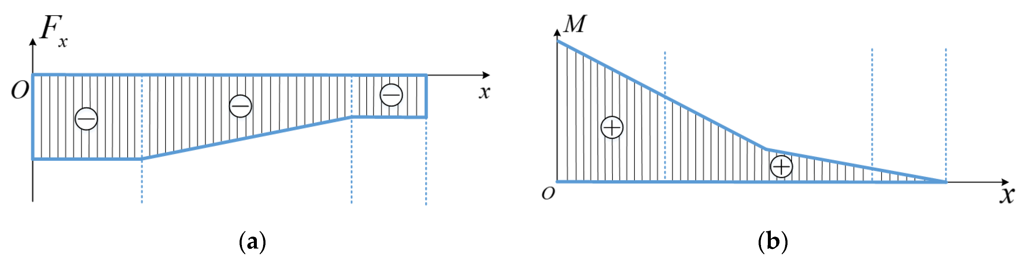
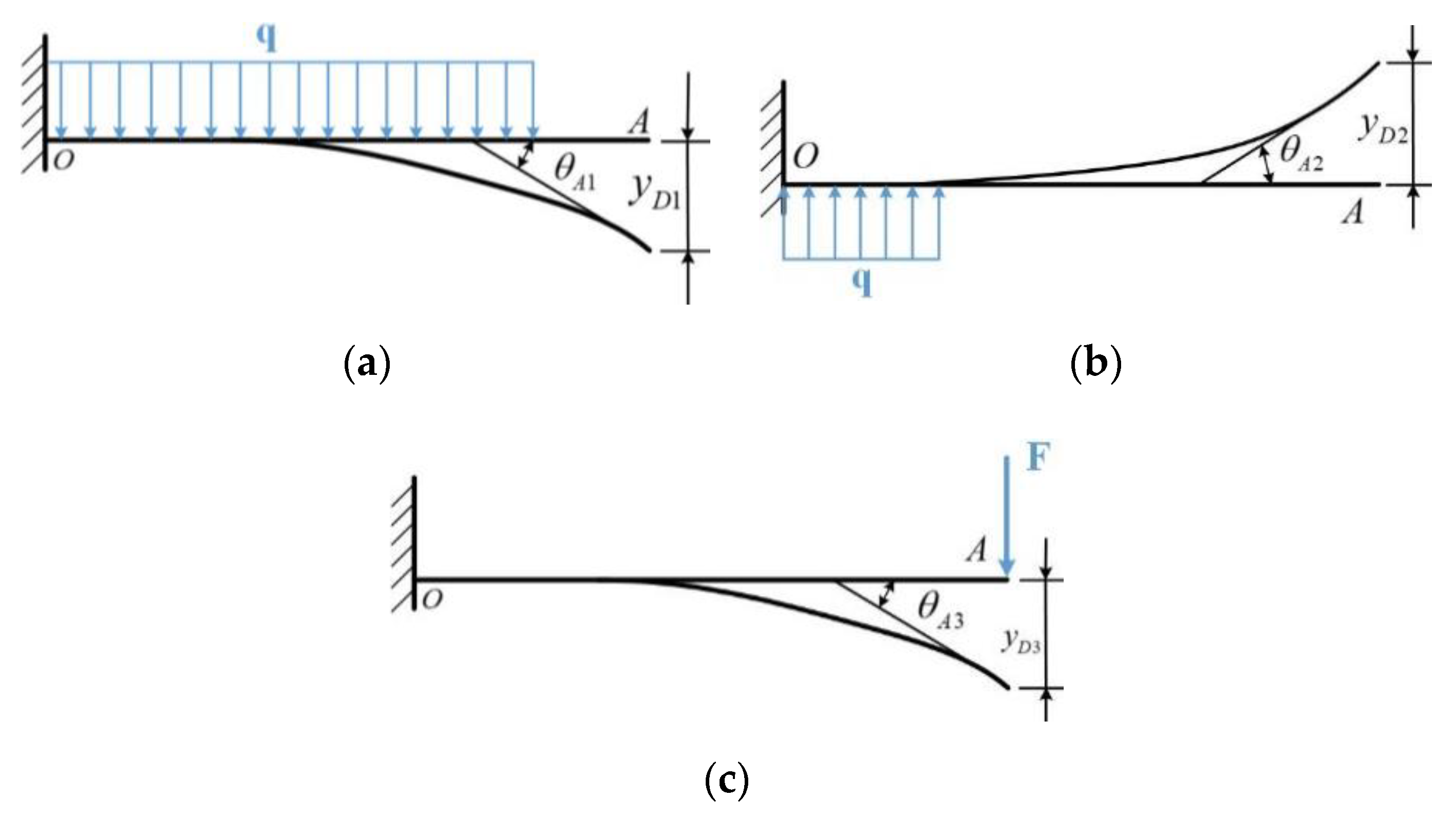
2.1. Bending Internal Force and Deflection
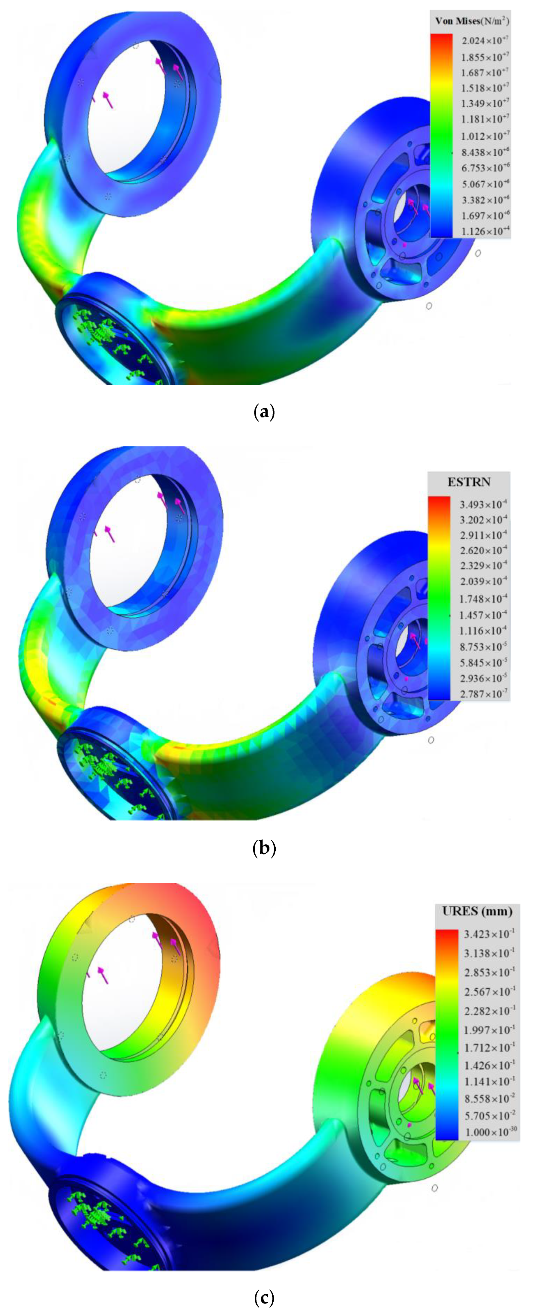
2.2. Finite Element Analysis
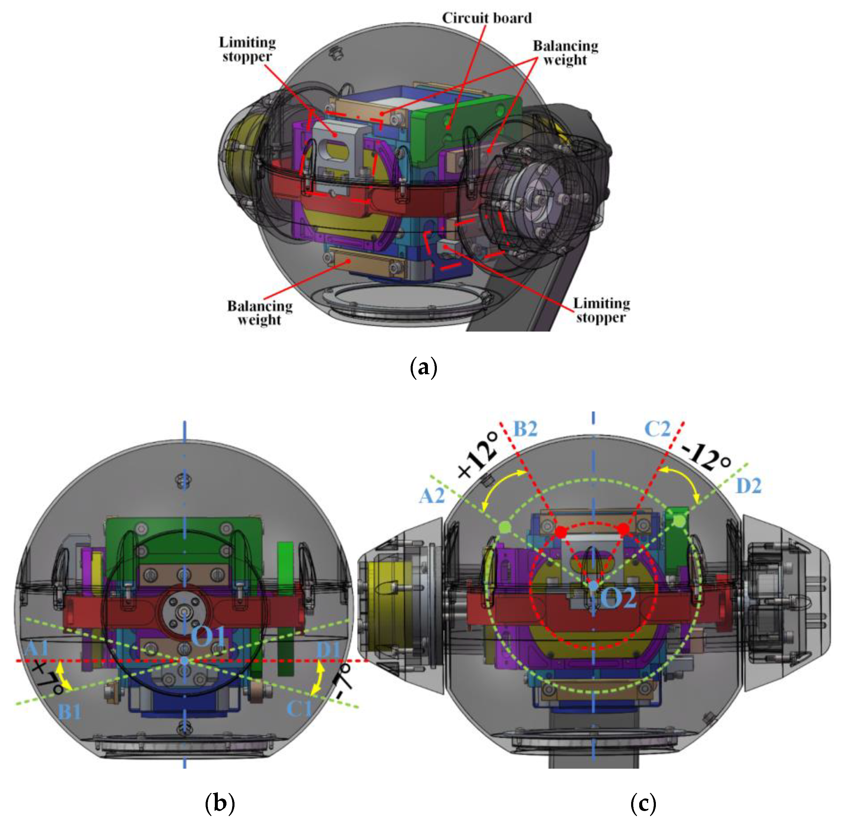
2.3. Design of Limit Structure of Rotation Angle
3. Dynamics Modeling
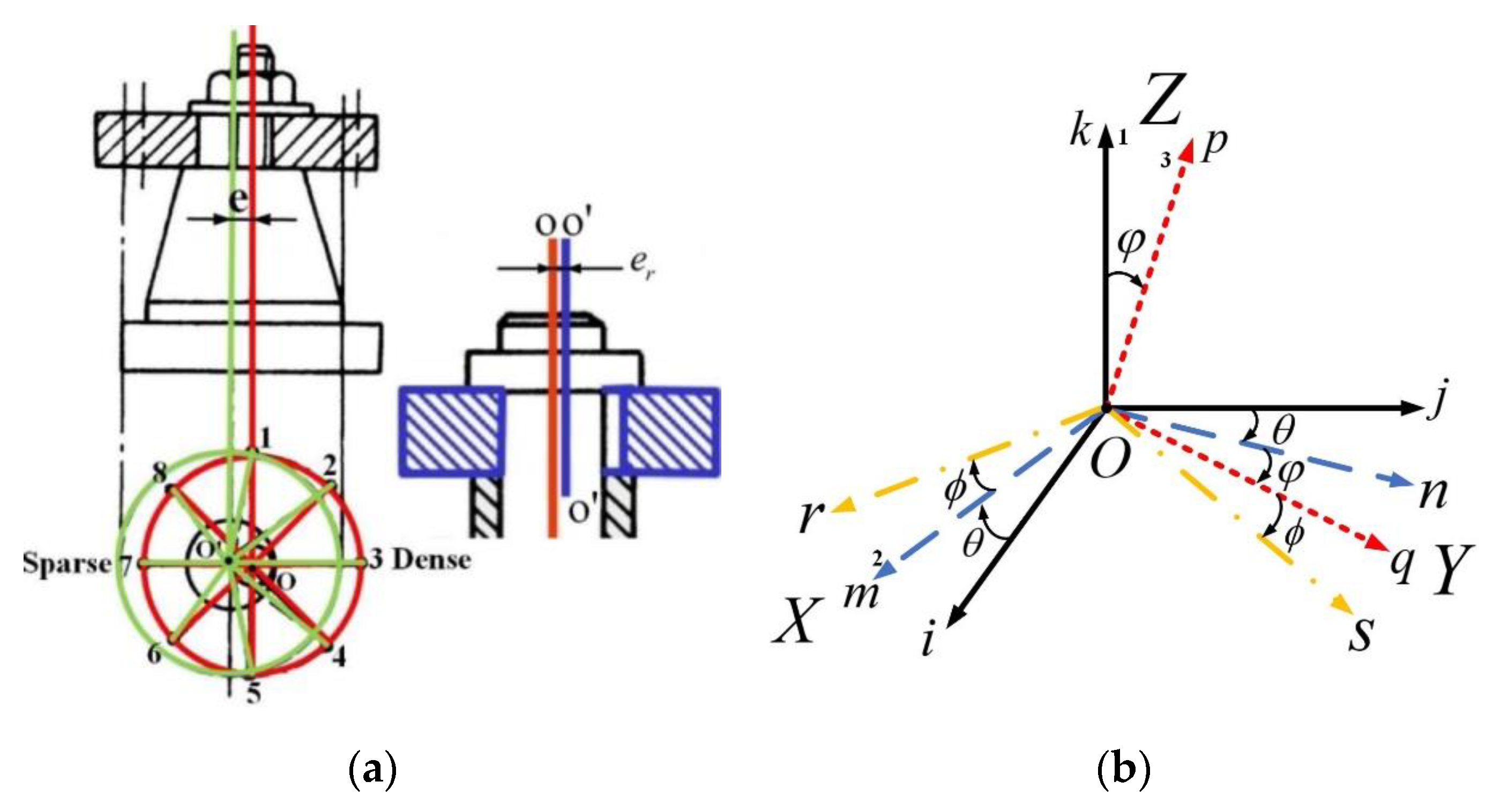
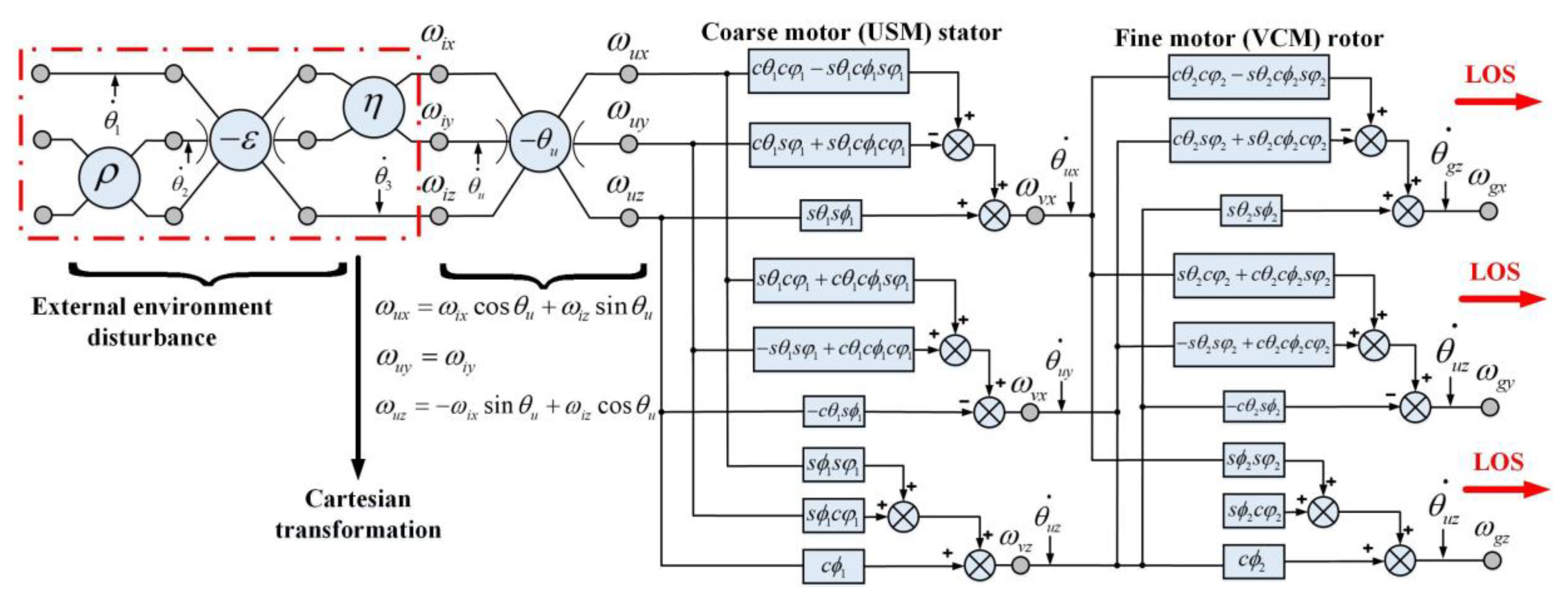
3.1. Coarse–Fine Composite Analysis
- A
- Inertial coordinate system ({i}, )
- B
- UAV coordinate system ({d}, )
- C
- Coarse motor stator coordinate system ({u}, )
- D
- Fine motor rotor coordinate system ({g}, )
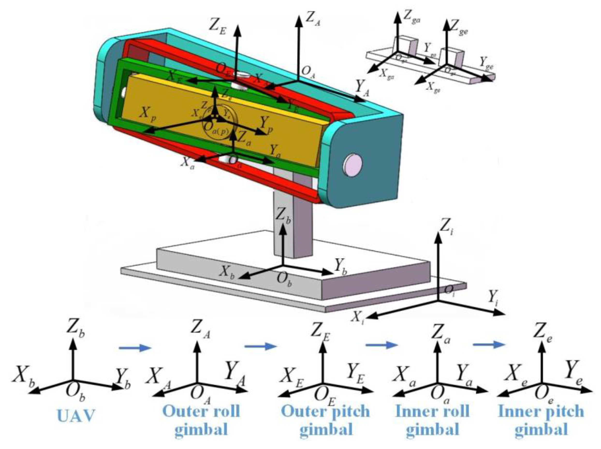
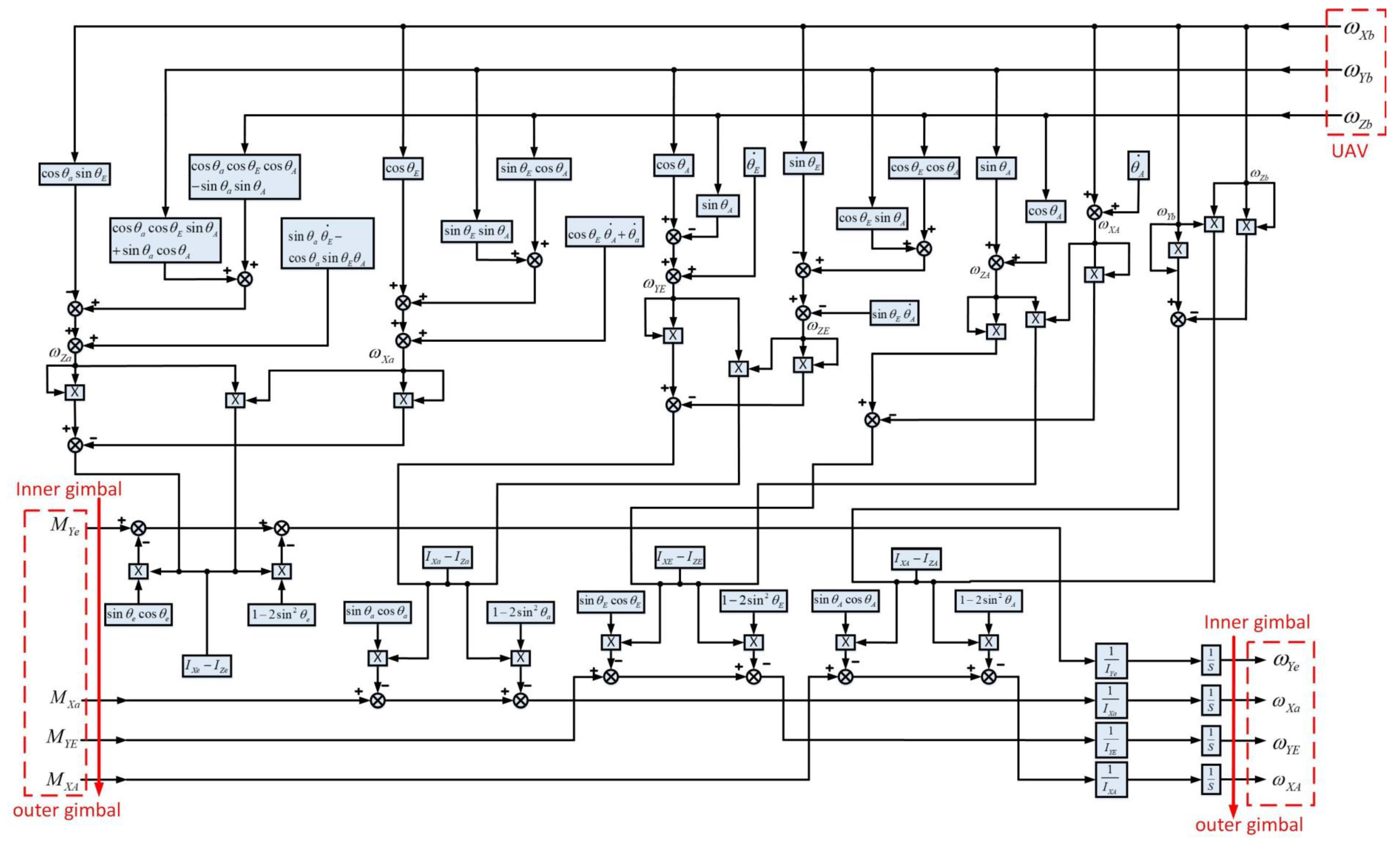
3.2. Two-Axis Four-Gimbal Structure
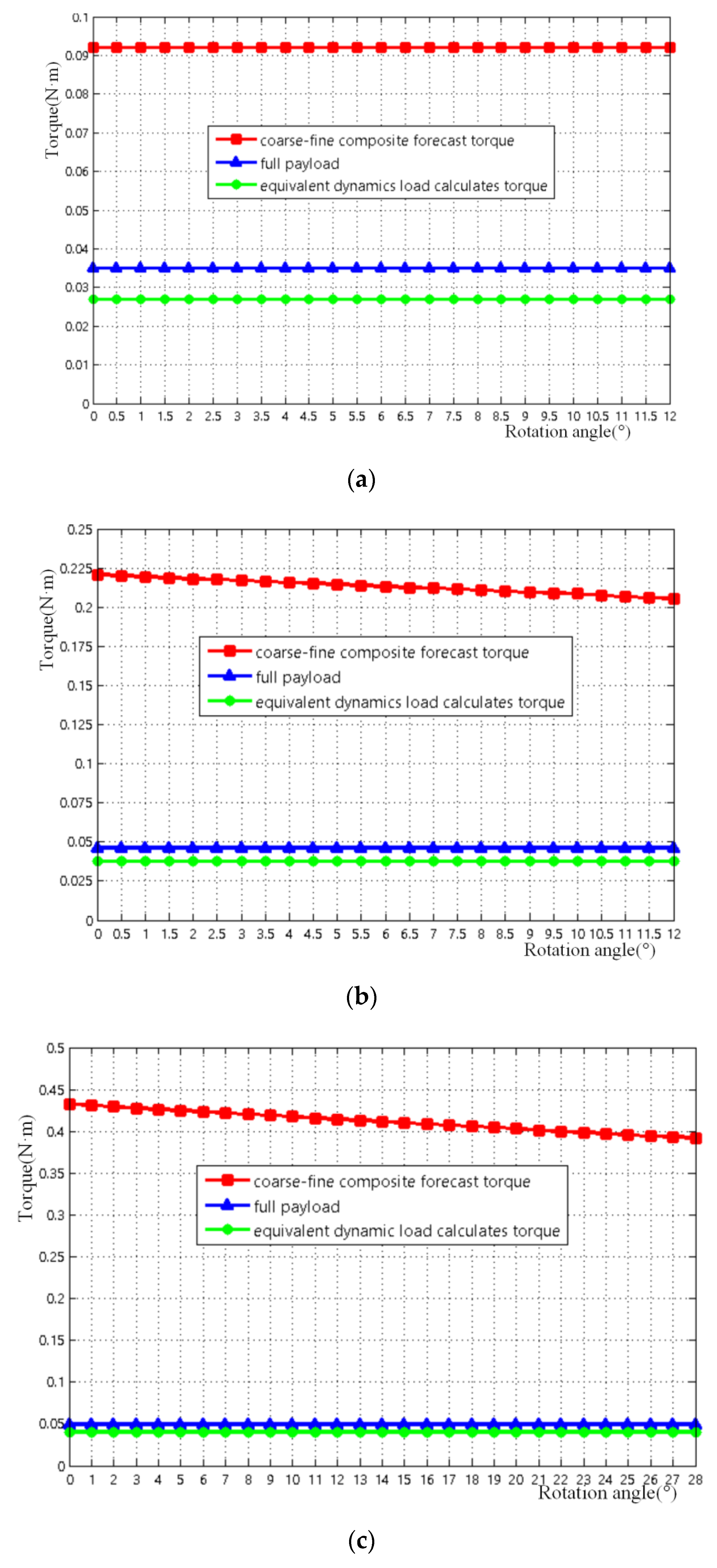
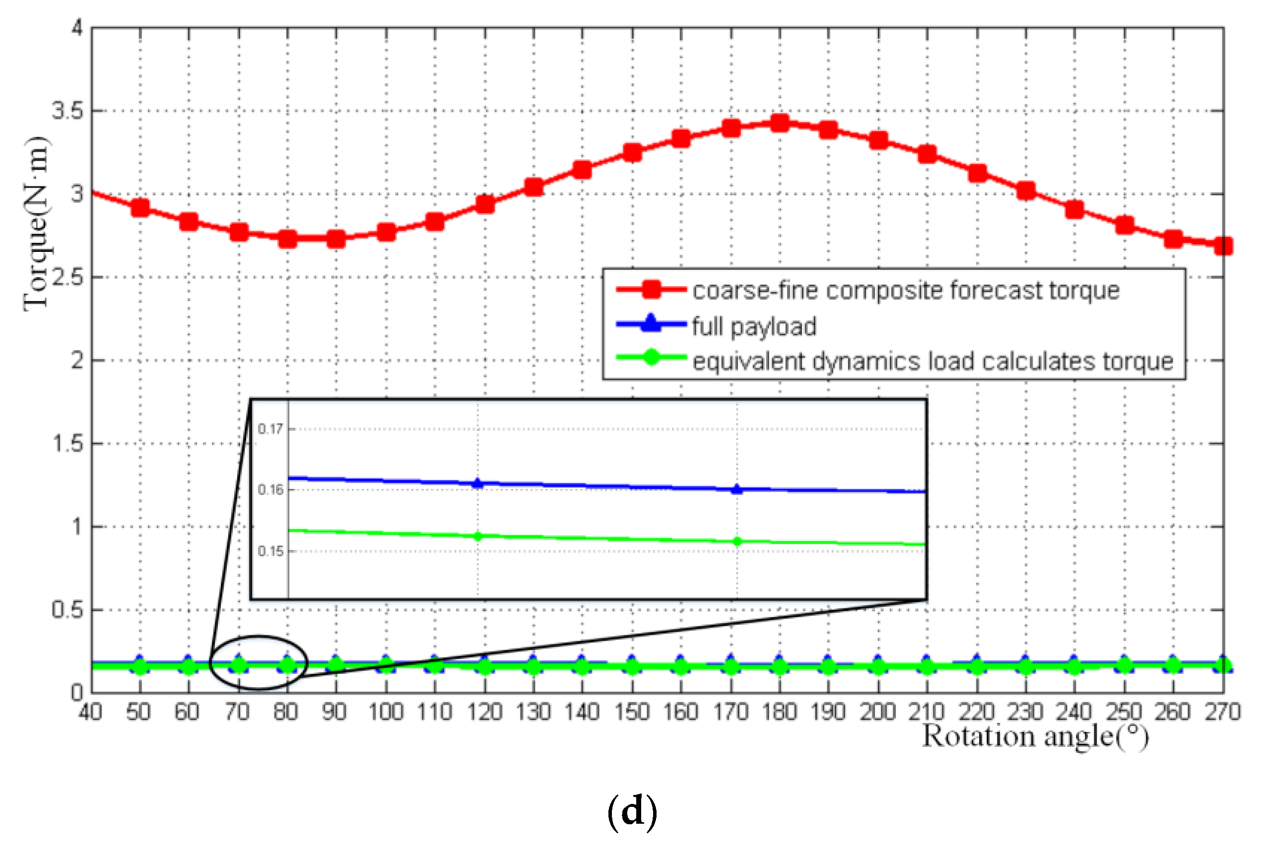
3.3. Comparison Validation
4. Experiment
5. Conclusions
- A
- In the UAV electro-optical pod of the two-axis four-gimbal, the characteristics of the coarse–fine composite structure and the complexity of dynamics modeling affect the entire system’s high-precision control performance. The core goal of this paper is solve the high precision control of two-axis four-gimbal electro-optical pod through dynamic modeling and theoretical study. FEA and theoretical analysis of the stress and deflection of the key structure component was used to design the structure. The gimbal structure adopts 7075-t3510 aluminum alloy, which is an aerospace material that meets the requirements of an ultralight electro-optical pod weighing less than 1 kg.
- B
- According to the Euler rigid body dynamics model, the transmission path and kinematics coupling compensation matrix for the two-axis four-gimbal are obtained. The coarse–fine composite drive correction equation of the inner-outer gimbals is derived to solve the pre-selection and check problem of the coarse–fine motors under high-precision control.
- C
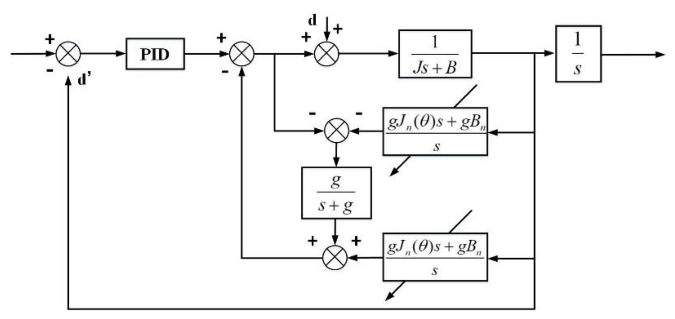
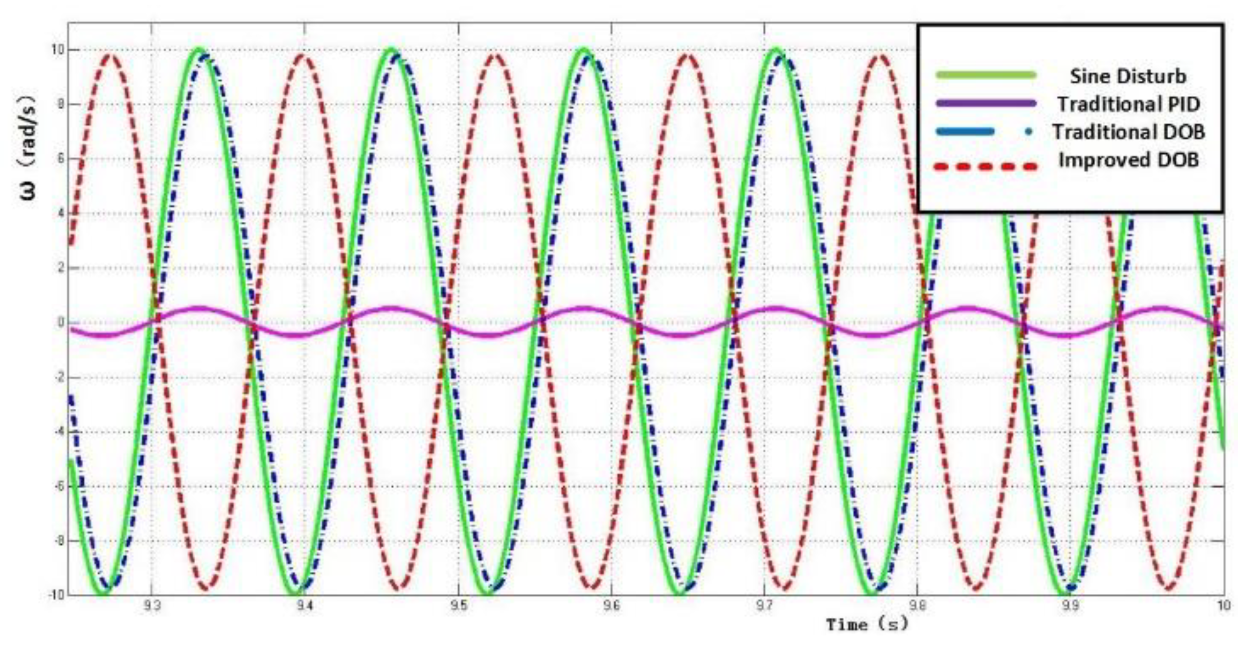
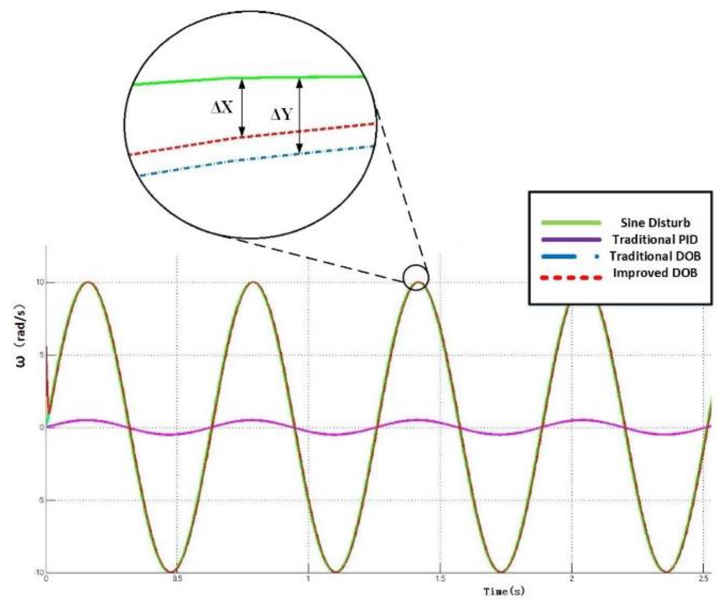
- The modeling method is substituted into the DOB disturbance suppression experiment, which can monitor and compensate for the motion coupling between gimbal structures in real time. Our results show that the disturbance suppression impact of the DOB method with dynamics model is up to 90% better than PID and 25% better than traditional DOB.
- D
- This manuscript is based on the dynamics modeling and theoretical study of the two-axis four-gimbal coarse–fine composite UAV electro-optical pod. This manuscript is valuable for all researchers interested in the coarse–fine composite, two-axis four-gimbal structures, and ultralight electro-optical pods.
Author Contributions
Funding
Acknowledgments
Conflicts of Interest
References
- Fan, D.P.; Zhang, Z.Y.; Fan, S.X.; Li, Y. Research of the basic principles of E-O stabilization and stabilization and tracking devices. Opt. Precis. Eng. 2006, 14, 673–680. [Google Scholar]
- Rue, A.K. Precision Stabilization Systems. IEEE Trans. Aerosp. Electron. Syst. 1974, AES-10. [Google Scholar] [CrossRef]
- Rue, A.K. Stabilization of precision electro-optical pointing and tracking systems. IEEE Trans. Aerosp. Electron. Syst. 1969, AES-5, 805–819. [Google Scholar] [CrossRef]
- Rue, A.K. Calibration of Precision Gimbaled Pointing Systems. IEEE Trans. Aerosp. Electron. Syst. 1970, AES-6, 697–706. [Google Scholar] [CrossRef]
- Rue, A.K. Correction to Stabilization of precision electro-optical pointing and tracking systems. IEEE Trans. Aerosp. Electron. Syst. 1970, AES-6, 855–857. [Google Scholar]
- Rue, A.K. Confidence Limits for the Pointing Error of Gimbaled Sensors. IEEE Trans. Aerosp. Electron. Syst. 1966, AES-2, 648–654. [Google Scholar]
- Preliasco, R.J. Wide-look-angle gimbal for an Airborne Electro-Optical Systems. Proc. SPIE 1998, 104–111. [Google Scholar] [CrossRef]
- Royalty, J. Development of Kinematics for Gimbaled Mirror and Prism Systems. SPIE 1990, 1304, 262–274. [Google Scholar]
- Kennedy, P.J.; Kennedy, R.L. Direct versus Indirect Line of Sight (LOS) Stabilization. IEEE Trans. Control Syst. Technol. 2003, 11, 3–15. [Google Scholar] [CrossRef]
- Zhao, L.J.; Dou, T.S.; Cheng, B.Q.; Xia, S.F.; Yang, J.X.; Zhang, Q.; Li, M.; Li, X.L. Theoretical Study and Application of the Reinforcement of Prestressed Concrete Cylinder Pipes with External Prestressed Steel Strands. Appl. Sci. 2019, 9, 5532. [Google Scholar] [CrossRef]
- Tomović, R. A Simplified Mathematical Model for the Analysis of Varying Compliance Vibrations of a Rolling Bearing. Appl. Sci. 2020, 10, 670. [Google Scholar] [CrossRef]
- Ma, P.F.; Li, Y.J.; Han, J.C.; He, C.; Xiao, W.K. Finite Element Modeling and Stress Analysis of a Six-Splitting Mid-Phase Jumper. Appl. Sci. 2020, 10, 644. [Google Scholar] [CrossRef]
- Harsh, D.; Shyrokau, B. Tire Model with Temperature Effects for Formula SAE Vehicle. Appl. Sci. 2019, 9, 5328. [Google Scholar] [CrossRef]
- Guo, L.D. Compound-Axis Macro-Micro Control and Modeling of Laser Weapon Tracking System. J. Jilin Univ. (Eng. Technol. Ed.) 2011, 41, 48. [Google Scholar]
- Choi, Y.M.; Gweon, D.G. A high-Precision Dual-Servo Stage Using Halbach Linear Active Magnetic Bearings. IEEE/ASME Trans. Mechatron. 2011, 16, 925–931. [Google Scholar] [CrossRef]
- Xia, Y.X.; Bao, Q.L.; Liu, Z.D. A New Disturbance Feedforward Control Method for Electro-Optical Tracking System Line-Of-Sight Stabilization on Moving Platform. Sensors 2018, 18, 4350. [Google Scholar] [CrossRef] [PubMed]
- Pio, R.L. Euler angle transformations. IEEE Trans. Autom. Control 1966, AC-I 1, 707–715. [Google Scholar] [CrossRef]
- Thomson, W.T. Introduction to Space Dynamics; Wiley: New York, NY, USA, 1963; pp. 101–108. [Google Scholar]
- Cong, J.W.; Tian, D.P.; Shen, H.H. Research on coupling self-correcting interference suppression control of airborne photoelectric platform. Electr. Mech. Eng. 2019, 36, 749–754. [Google Scholar]
- Chen, X.G.; Cai, M.; Dai, N. Disturbance suppression method of airborne photoelectric stabilized platform based on DOB observer. Electro-Optic Control 2019, 11, 1–6. [Google Scholar]


| Length | Value/mm |
|---|---|
| 40 | |
| 43 | |
| 33 | |
| Span H | 116 |
| Parameter | Value |
|---|---|
| F | 0.00022 kN |
| q | 0.0085 kN/m |
| Parameter | Value | |
|---|---|---|
| Max | Min | |
| Stress | ||
| Strain | ||
| Displacement | ||
| The deformation ratio | 49.3719 | |
| Gimbal | Rotational Inertia (Including Load/kg·m2) | Mass (Including Load/kg) | ||
|---|---|---|---|---|
| X | Y | Z | ||
| Inner pitch e | 0.471 | |||
| Inner roll a | 0.681 | |||
| Outer pitch E | 0.740 | |||
| Outer roll A | 1.925 | |||
© 2020 by the authors. Licensee MDPI, Basel, Switzerland. This article is an open access article distributed under the terms and conditions of the Creative Commons Attribution (CC BY) license (http://creativecommons.org/licenses/by/4.0/).
Share and Cite
Shen, C.; Fan, S.; Jiang, X.; Tan, R.; Fan, D. Dynamics Modeling and Theoretical Study of the Two-Axis Four-Gimbal Coarse–Fine Composite UAV Electro-Optical Pod. Appl. Sci. 2020, 10, 1923. https://doi.org/10.3390/app10061923
Shen C, Fan S, Jiang X, Tan R, Fan D. Dynamics Modeling and Theoretical Study of the Two-Axis Four-Gimbal Coarse–Fine Composite UAV Electro-Optical Pod. Applied Sciences. 2020; 10(6):1923. https://doi.org/10.3390/app10061923
Chicago/Turabian StyleShen, Cheng, Shixun Fan, Xianliang Jiang, Ruoyu Tan, and Dapeng Fan. 2020. "Dynamics Modeling and Theoretical Study of the Two-Axis Four-Gimbal Coarse–Fine Composite UAV Electro-Optical Pod" Applied Sciences 10, no. 6: 1923. https://doi.org/10.3390/app10061923
APA StyleShen, C., Fan, S., Jiang, X., Tan, R., & Fan, D. (2020). Dynamics Modeling and Theoretical Study of the Two-Axis Four-Gimbal Coarse–Fine Composite UAV Electro-Optical Pod. Applied Sciences, 10(6), 1923. https://doi.org/10.3390/app10061923