The Spatiotemporal Variability of Temperature and Precipitation Over the Upper Indus Basin: An Evaluation of 15 Year WRF Simulations

Abstract

Investigating the trends in the major climatic variables over the Upper Indus Basin (UIB) region is difficult for many reasons, including highly complex terrain with heterogeneous spatial precipitation patterns and a scarcity of gauge stations. The Weather Research and Forecasting (WRF) model was applied to simulate the spatiotemporal variability of precipitation and temperature over the Indus Basin from 2000 through 2015 with boundary conditions derived from the Climate Forecast System Reanalysis (CFSR) data. The WRF model was configured with three nested domains (d01–d03) with horizontal resolutions increasing inward from 36 km to 12 km to 4 km horizontal resolution, respectively. These simulations were a continuous run with a spin-up year (i.e., 2000) to equilibrate the soil moisture, snow cover, and temperature at the beginning of the simulation. The simulations were then compared with TRMM and station data for the same time period using root mean squared error (RMSE), percentage bias (PBIAS), mean bias error (MBE), and the Pearson correlation coefficient. The results showed that the precipitation and temperature simulations were largely improved from d01 to d03. However, WRF tended to overestimate precipitation and underestimate temperature in all domains. This study presents high-resolution climatological datasets, which could be useful for the study of climate change and hydrological processes in this data-sparse region.

1. Introduction

The Himalaya-Karakoram-Hindukush (HKHK) region has significant strategic importance due to large amounts of snow and glacial ice [1]. Often referred to as Earth’s “third pole” [2] (to indicate its massive ice and snow storage comparable to the North and South poles), it provides freshwater supply for agriculture, energy production, and drinking purposes for 1.5 billion people living in its catchments [3]. The HKHK region is also hydrologically important due to the presence of major rivers such as the Indus, Ganges, and Brahmaputra.

The Indus Basin Irrigation System (IBIS) is one of the largest irrigation systems in the world, which supports not only over 90% of Pakistan’s agricultural production [3], but also the majority of the water needs for Pakistan [4]. Over the catchment area up to the Tarbella Reservoir (known as UIB), the contribution from snow and glacier melt runoffs accounts for about 70–80%, and the Karakoram Mountains alone contribute to more than 50% of runoff [3]. Despite the hydrological importance, there is no consensus on the assessment of the stability of the glaciers in the region. Previous studies have shown conflicting results for glaciers located in the Karakoram ranges, concluding that they are stable, retreating, or even advancing (the so-called Karakoram Anomaly [5,6]). The Indus River Basin (IRB) has experienced increasing temperatures and features immense spatial variability in climate [7].

Because the Indus River is largely dependent on cryosphere melt, it is highly vulnerable to climate change [8]. The Global Climate Risk Index (CRI) 2018 [9] has ranked Pakistan in the top ten countries most affected by climate change. Global climate models (GCMs) are the basic tools to simulate and project climate change, but their low spatial resolution makes them unable to resolve mesoscale flow patterns [10]. Several studies have downscaled GCM simulations over the IRB (for example, [11,12,13]); they found that temperature will continue to increase, but precipitation will be highly uncertain over this region. In addition, GCMs do not have the capability to resolve the orographic precipitation in complex mountainous regions such as UIB. This uncertainty in projected changes in climatic variables, especially precipitation, causes substantial uncertainty in runoff estimations.

In addition, the UIB is a data-scarce region where very few rain gauges are installed. These gauges are unevenly distributed and primarily at low-elevation valley locations, raising concerns about their representativeness of higher elevation orographic effects [14]. The lack of sufficient meteorological observations is usually the most challenging for flood forecasting and water resources management over this region. Complex topography, coupled with the challenges of field study in this region, has led to considerable uncertainty in assessing glacial mass balance and even meteorological trends. Moreover, the available global reanalysis datasets are useful to assess the large scale flow patterns over this region, but their coarse resolution cannot effectively characterize the complex orography and other local dynamics [14,15].

Regional climate models such as the Advanced Research Weather Research & Forecasting model (ARW-WRF; hereafter WRF) can be applied to simulate climatic parameters in complex terrain at high resolution. High-resolution atmospheric modeling can fill the gap of observational data scarcity to advance the understanding of atmospheric variability. The WRF model has successfully been applied worldwide [16,17,18,19,20] and to the Tibetan Plateau [21,22,23,24,25]. Gao et al. [25] applied the WRF model to perform 32 years (1979–2011) of simulations over the Tibetan Plateau at 30 km grid cell resolution, but this resolution is still somewhat coarse for capturing orographic precipitation patterns [23]. Maussion et al. [14] also used the WRF model to perform 11 years (October 2000–September 2011) of simulations over the Tibetan Plateau at 30 km and 10 km grid cell resolution in the outer and inner domain, respectively. Norris et al. [15] emphasized the importance of finer grid cell resolution over this region to simulate climatic variables, especially precipitation. However, investigating the long-term high-resolution meteorological variability (at 4 km) over the Karakoram Mountain Range is lacking, which is very important for the glaciological and hydrological communities.

In view of the above, we used the WRF model Version 3.8.1 [26] to dynamically downscale 16 years (2000–2015) over the Indus Basin. Our purpose in this study is to investigate spatiotemporal variability in the climate over the UIB and to assess the ability of WRF to capture observed variations using an analysis of correlation, bias, and trend. Potential issues with robustness stemming from record length are captured in our results via rigorous significance testing on all trends. The WRF model has been configured with three nested domains (d01–d03) with the boundary conditions derived from the National Oceanic and Atmospheric Administration (NOAA) National Center of Environmental Prediction (NCEP) 6 hourly Climate Forecast System Reanalysis (CFSR) data [27], which has a 38 km horizontal resolution. This study provides an analysis of the WRF model’s applicability over the complex terrain of the UIB at an annual and seasonal scale.

2. Materials and Methods

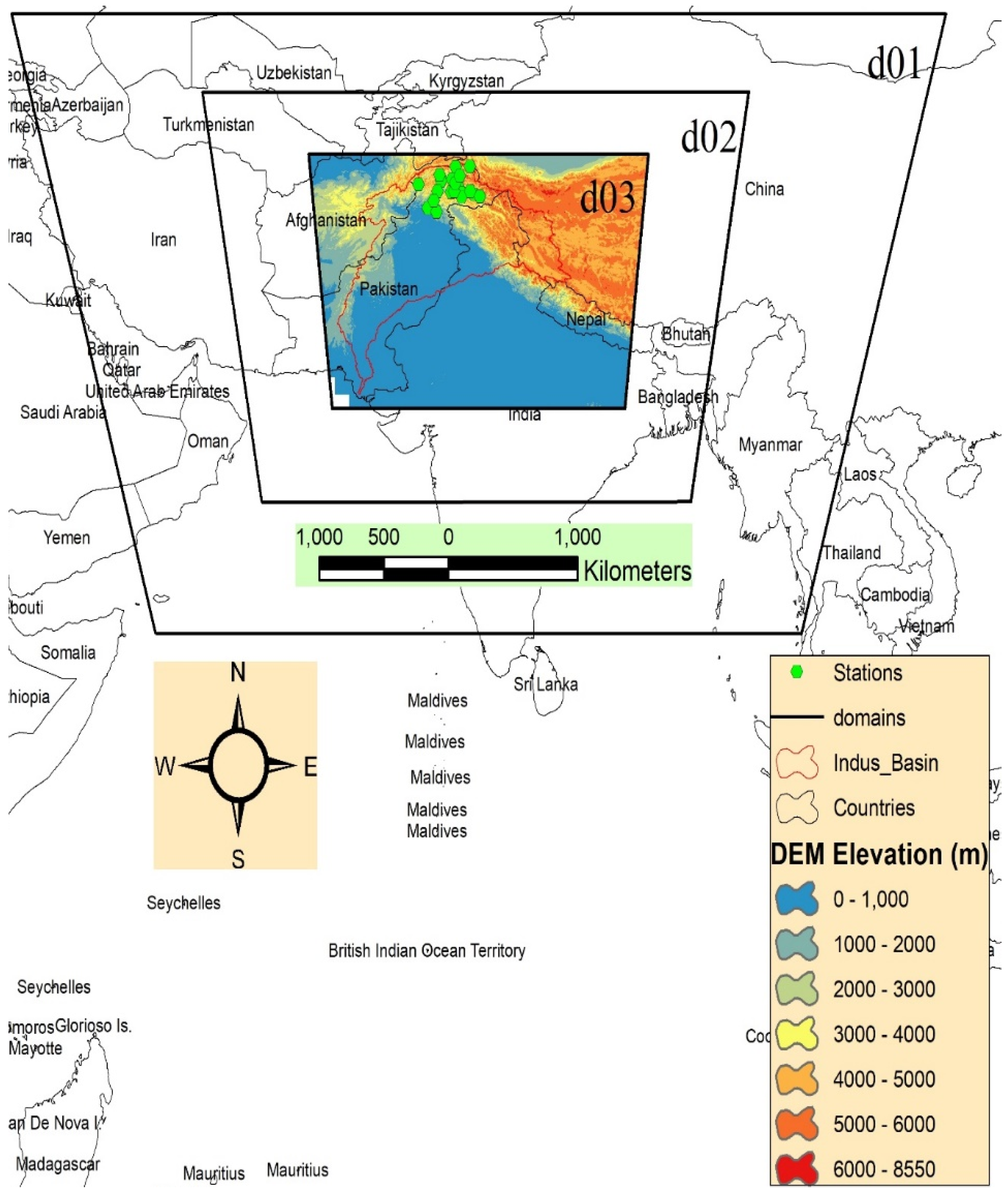
2.1. Study Area

This study had three domains with different scales and grid cell resolutions. The northern parts of the Indus River consist of high mountains, including the HKHK mountain ranges, whereas its southern parts consist of flat plains. The inner domain (d03) covered the whole Indus Basin (Figure 1), but this study is focused on the Upper Indus Basin (UIB). The climate in the northern parts (UIB) is largely influenced by western disturbances, and this region receives most of the precipitation (i.e., up to 2000 mm) in the winter season [28,29]. However, the precipitation in the Lower Indus Basin (southern parts) is driven by the monsoon precipitation in the summer season, which ranges from 100 to 500 mm [30,31]. In the UIB, the mean monthly temperature varies from 2 to 49 °C, whereas in the Lower Indus Basin, the mean monthly temperature varies from 14 to 44 °C [30]. The elevation of this study region varies from 0 to 8550 m above sea level, which has been derived from a 90 m resolution digital elevation model (DEM) from the Shuttle Radar Topography Mission (SRTM) project. The UIB is a high altitude and complex mountainous area wherein the Karakoram Mountain Ranges and the Hindu Kush and Himalayan Mountains are located. Typically, three major factors may influence the climate over this region: the winter westerlies, the summer monsoon, and a high-pressure system formed over high Asia [32]. Most of the precipitation over this region occurs in winter and spring and is influenced by winter westerly flow [33].

2.2. WRF Model Configuration

The Advanced Research Weather Research & Forecasting model (ARW-WRF, hereafter WRF) Version 3.8.1 [26] was used to downscale 16 years (2000–2015) of CFSR data dynamically [27], which have approximately a 38 km horizontal grid resolution. These simulations were a continuous run with a spin-up year (i.e., 2000) to equilibrate the soil moisture, snow cover, and temperature at the beginning of the simulation. The motivation for using CFSR data in this study was taken from Bao and Zhang [34], wherein they evaluated several datasets over the Tibetan Plateau. They found CFSR and the Interim European Center for Medium-Range Weather Forecasts (ECMWF) reanalysis datasets (ERA-Interim) to simulate atmospheric changes effectively. They showed that both datasets presented smaller RMS error and mean bias. The main reason for selecting the CFSR dataset, specifically in this study, was its resolution. The CFSR dataset had a higher spatial resolution (0.5° by 0.5°) than ERA-Interim (0.75° by 0.75°).

The WRF model used in this study was configured with three nested domains with gradually increasing horizontal resolution from 36 km through 12 km to convection-permitting 4 km so that the innermost domain did not rely on a cumulus parameterization. The model configuration presented in Figure 1 was specifically chosen to limit the influence of boundary conditions on the results by assuring large margins between the nested domains. In addition, the relaxation zone of five points used in this study was very small compared to the domain sizes. The choice of the innermost domain size stemmed from work by Norris et al. [15], who emphasized that a fine grid cell resolution was required to resolve orographic precipitation in this region. The detailed model strategy and parametrization schemes used in this study are given in

Table 1. Model strategy. d01, Domain 01.

A. Physical parameterization schemes
Land surface model (LSM)	Noah multi-parameterization (Noah-MP) [35]
Planetary boundary layer (PBL)	Yonsei University (YSU) scheme [36]
Microphysics	Thompson microphysics scheme [37]
Longwave radiation	Rapid radiative transfer model (RRTM) [38]
Shortwave radiation	Dudhia scheme [39]
Surface Layer	Revised MM5 scheme [40]
Cumulus parameterization	Kain–Fritsch scheme [41] in d01 and d02
B. Grids and Nesting Strategy
Nesting	Two-way nesting; Nested in a cascade approach (d01-d02-d03)
Horizontal grid cell resolution	d01 36 km resolution (146 × 115) d02 12 km resolution (270 × 219) d03 4 km resolution (526 × 403)
Map projection	Lambert conformal
Number of vertical layers	38
Top-level pressure	10,000 Pa
Center point of domains	30.75°N, 76.00°E
Timestep	Parent time step ratio of 1:3 120 s in d01, 40 s in d02, and 13.33 s in d03
Size of domains	Outer domain (d01) has 146 by 115 grid spaces; middle domain (d02) has 271 by 220 grid spaces; inner domain (d03) has 526 by 403 grid spaces
C. Sensitivity Analysis
Simulation 1	Thompson and Noah-MP
Simulation 2	Morrison and Noah-MP
Simulation 3	Goddard and Noah-MP
Simulation 4	Thompson and CLM4

.

Research showed that WRF was highly sensitive to the selection of the land surface model (LSM) and cloud microphysical scheme [15]. Based on limited computational resources, four simulation experiments (Table 1. Section C) were performed for the year 2004 with a combination of three cloud microphysical schemes (Thompson, Morrison, and Goddard) and two land surface models (Noah-multi-parameterization (Noah-MP) and (Community Land Model version 4 (CLM4)) over the UIB. The RMS error and Pearson’s r between WRF, stations, and TRMM data were estimated at Skardu station for the year 2004. The results showed that the RMS error between the WRF and station data was lower in all three domains in Simulation 1. In addition, Pearson’s r between the WRF and station data in Simulation 1 was slightly higher than the other three simulations. Therefore, the results suggested that out of the tested configuration, Simulation 1 (Thompson and Noah-MP) offered the best performance. This was also consistent with Norris et al. [15], wherein they performed sensitivity analysis over the same region for selected summer and winter days.

2.3. Model Validation

We evaluated the WRF temperature and precipitation output with the station meteorological data collected from the Pakistan Meteorological Department (PMD) and Water and Power Development Authority (WAPDA) (details of the stations are given in

Table 2. PMD stations, their locations, elevation, and the respective domain. PMD, Pakistan Meteorological Department; WAPDA, Water and Power Development Authority. P and T represent precipitation and average temperature, respectively.

Station	Lat	Lon	Station Elevation (m)	Data	Data Range	Source
Astore	35.33	74.90	2168	P, T	2000–2014	PMD
Bunji	35.67	74.63	1372	P, T	2000–2014	PMD
Chillas	35.42	74.10	1250	P, T	2000–2014	PMD
Chitral	35.85	71.83	1497	P, T	2000–2014	PMD
Gilgit	35.92	74.33	1460	P, T	2000–2014	PMD
Gupis	36.17	73.40	2156	P, T	2000–2014	PMD
Hunza	36.32	74.65	2156	P, T	2007–2014	PMD
Skardu	35.30	75.68	2317	P, T	2000–2014	PMD
Khunjerab	36.85	75.40	4707	P, T	2000–2015	WAPDA
Rama	35.36	74.81	3140	P, T	2000–2012	WAPDA
Rattu	35.15	74.82	2920	P, T	2000–2015	WAPDA
Ushkore	36.03	73.40	3353	P	2000–2015	WAPDA
Yasin	36.37	73.30	3353	P	2000–2015	WAPDA
Ziarat	36.83	74.42	3688	P	2000–2015	WAPDA
Naltar	36.13	74.18	2810	P	2000–2015	WAPDA
Ganji	35.45	74.31	1576	P	2000–2015	WAPDA
Daggar	34.51	72.49	732	P	2005–2015	WAPDA
Kachura	35.45	75.42	2340	P	2005–2015	WAPDA
Kandia	35.47	73.15	858	P	2005–2015	WAPDA
Karimabad	36.33	74.70	3048	P	2005–2015	WAPDA
Phulra	34.31	73.08	915	P	2005–2015	WAPDA
Yugo	35.18	76.10	2469	P	2005–2015	WAPDA
Besham Qila	34.93	72.88	580	P	2005–2015	WAPDA

). We evaluated the WRF temperature with the available data of ten stations (Table 2) for the time period of 2001 through 2010. Similarly, the stations’ data for precipitation were not available for the entire simulation period. Because of the limited availability of station data, we also assessed the WRF precipitation output with the Tropical Rainfall Measuring Mission (TRMM) 3B42 Version 7 gridded precipitation data [42] at a monthly temporal scale. The TRMM 3B42V7 data were available on a 0.25° by 0.25° latitude-longitude grid at 3 hourly temporal resolution. TRMM 3B42V7 data were collected from remote sensing and adjusted based on the monthly gauge data. Despite its coarse resolution and other limitations, TRMM 3B42V7 is considered to be one of the reliable gridded precipitation datasets [4,15]. Krakauer et al. [4] compared different precipitation datasets with the available stations’ data over the Indus Basin and found the TRMM dataset to perform best among the remote sensing datasets. Similarly, Ali et al. [43] evaluated the TRMM Multi-satellite Precipitation Analysis (TMPA) precipitation products (3B42V6, 3B42V7, and 3B42RT) with gauge stations over the Hunza Basin in Karakoram Mountainous range. They also found 3B42V7 reasonably better than the other two products. Several studies have also evaluated the WRF precipitation with the TRMM dataset (for example, [14,15]).

The WRF precipitation output was evaluated by the root mean squared error (RMSE), percentage bias, and Pearson correlation coefficient (r), whereas WRF temperature output was evaluated by RMSE, mean bias, and Pearson correlation coefficient. The expressions of RMSE, percentage bias (PBIAS), and mean bias for n grid points or n stations are:

$$RMSE=\sqrt{\frac{1}{n}{\displaystyle \sum }_{i=1}^n{\left(M_i-O_i\right)}^2},$$

(1)

$$PBIAS=\frac{1}{n}{\displaystyle \sum }_{i=1}^n(\left(M_i-O_i\right)/O_i)\ast 100,$$

(2)

$$meanbias=\frac{1}{n}{\displaystyle \sum }_{i=1}^n\left(M_i-O_i\right)$$

(3)

where $M_i$ and $O_i$ represent model simulations and observed data, respectively.

2.4. Trend Analysis

In this study, we performed a trend analysis using the Mann–Kendall (MK) significance test [44,45]. It is a non-parametric test and less affected by the extreme values, which is also widely used to detect trends in hydrologic time series [46,47].

3. Results

In this section, we evaluate the simulated precipitation in the three domains using the PMD meteorological data and TRMM data. However, the simulated temperature was evaluated only using the PMD meteorological data.

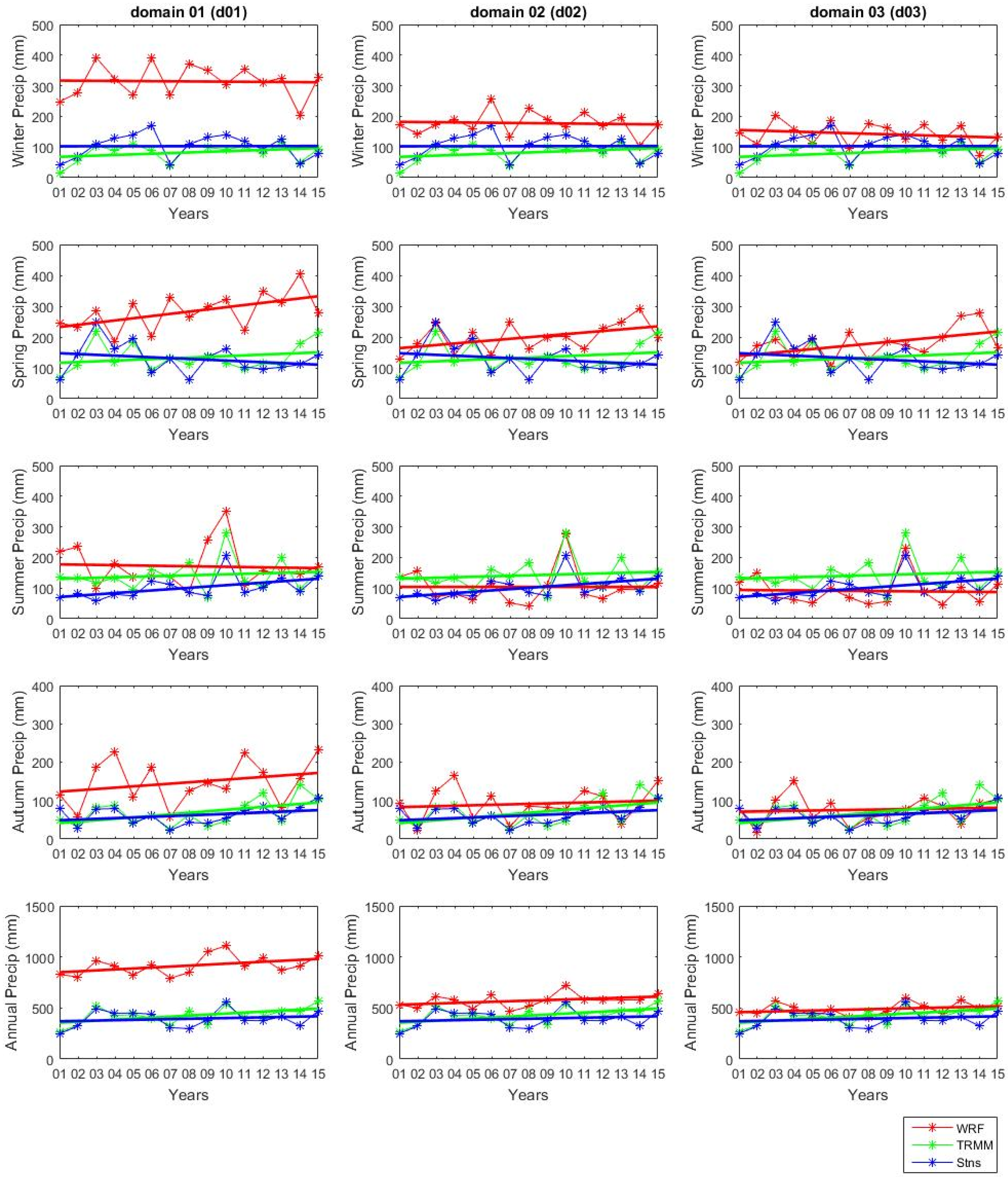
3.1. Station-averaged Precipitation Trends

This section describes the extent to which WRF was accurate in reproducing the spatio-temporal variability of precipitation in the three domains. The annual and seasonal mean precipitation trends for WRF, TRMM, and station data for all domains are shown in Figure 2. In addition, the Pearson correlation coefficient was computed between WRF and both observed datasets.

There were twenty-three stations (given at Table 2) operated by PMD and WAPDA above Tarbella Reservoir, and WRF and TRMM data were interpolated at these stations. When WRF, TRMM, and gauge data at these stations were averaged and compared in d01, WRF tended to overpredict the total annual precipitation relative to TRMM (115%) and the gauge data (132%) (left column, Figure 2). In addition, the results showed that the winter season had more bias (PBIAS—206%; RMSE—214 mm) and the summer season had less bias (PBIAS—70%; RMSE—91 mm) to the stations’ data in the outer domain. For seasonal precipitation variation from 2001 to 2015, WRF showed a positive correlation with TRMM and station data for all seasons (

Table 3. Mean RMSE (mm), percentage difference (%), and Pearson correlation coefficient (r; unitless) of precipitation between WRF, stations, and TRMM in d01, d02, and d03.

		d01	d02	d03
Winter (DJF)	RMSE (mm) btw WRF and Station (WRF and TRMM)	214 (235)	81 (101)	53 (69)
	PBIAS (%) btw WRF and Station (WRF and TRMM)	206 (282)	73 (116)	39 (74)
	Pearson Correlation coefficient (r) btw WRF and Station (WRF and TRMM)	0.67 (0.69)	0.7(0.53)	0.59 (0.55)
Spring (MAM)	RMSE (mm) btw WRF and Station (WRF and TRMM)	169 (169)	89 (77)	78 (67)
	PBIAS (%) btw WRF and Station (WRF and TRMM)	119 (112)	55 (50)	38 (34)
	Pearson Correlation coefficient (r) btw WRF and Station (WRF and TRMM)	0.08 (0.41)	0.34 (0.58)	0.22 (0.44)
Summer (JJA)	RMSE (mm) btw WRF and Station (WRF and TRMM)	91 (72)	42 (59)	36 (62)
	PBIAS (%) btw WRF and Station (WRF and TRMM)	70(21)	3 (−26)	−10 (−36)
	Pearson Correlation coefficient (r) btw WRF and Station (WRF and TRMM)	0.51 (0.39)	0.67 (0.63)	0.7 (0.75)
Autumn (SON)	RMSE (mm) btw WRF and Station (WRF and TRMM)	95 (90)	39 (39)	25 (29)
	PBIAS (%) btw WRF and Station (WRF and TRMM)	138 (117)	47(34)	23 (12)
	Pearson Correlation coefficient (r) btw WRF and Station (WRF and TRMM)	0.79 (0.67)	0.82 (0.64)	0.69 (0.65)
Annual	RMSE (mm) btw WRF and Station (WRF and TRMM)	525 (497)	185 (160)	111 (91)
	PBIAS (%) btw WRF and Station (WRF and TRMM)	132 (115)	45 (35)	23 (15)
	Pearson Correlation coefficient (r) btw WRF and Station (WRF and TRMM)	0.66 (0.52)	0.74 (0.63)	0.67 (0.59)

). Similarly, WRF annual precipitation was significantly correlated with TRMM and gauge data (p < 0.05). However, trend analyses for WRF, TRMM, and gauge stations located in d01 did not show any statistically significant trends except the summer season, where station data showed a statistically significant trend. Moreover, the annual TRMM showed a statistically significant trend.

When WRF and TRMM data were interpolated at the twenty-three gauge locations in d02 and compared, WRF still overpredicted total annual precipitation compared with the TRMM (35%) and gauge data (45%) (middle column, Figure 2). In addition, the results showed that the winter season had more bias (73%) and the summer season had less bias (3%) to the stations’ data in the middle domain. WRF was significantly correlated with TRMM and gauge stations (p < 0.05) in all seasons except spring, where WRF was positively, but not significantly correlated with the station data. However, trend analyses for WRF, TRMM, and gauge stations located in d02 did not show any statistically significant trends except the summer season, where station data showed a statistically significant trend. Moreover, the annual TRMM showed a statistically significant trend.

When WRF and TRMM data were interpolated at the twenty-three gauge locations in d03 and compared, WRF still overpredicted total annual precipitation compared with TRMM (15%) and gauge data (23%) (right column, Figure 2). In addition, the results showed that the winter season had more bias (39%) and the summer season has less bias (−10%) to the stations’ data in the inner domain (Table 3). Moreover, WRF was significantly correlated with TRMM and gauge stations (p < 0.05) in all seasons except spring, where WRF was positively, but not significantly correlated with the station and TRMM data. However, trend analyses for WRF, TRMM, and gauge stations located in d03 did not show any statistically significant trends except the summer season, where station data showed a statistically significant trend. Moreover, the annual TRMM showed a statistically significant trend.

The station-wise comparison of PBIAS (

Table 4. PBIAS of precipitation and mean bias (°C) of T2 after lapse rate correction between WRF and stations in d01, d02, and d03 at an annual time scale.

	PBIAS			Mean Bias (°C)
Station	d01	d02	d03	d01	d02	d03
Astore	135	54	42	−3.4	−1.5	0.76
Bunji	329	47	−3.5	−9.8	−2.6	4.7
Chillas	213	19	24	−13.6	−4.0	−0.2
Chitral	111	27	−3	−12.8	−6.8	−3.7
Gilgit	447	141	42	−12.2	−7.1	0.4
Gupis	257	103	184	−14.9	−11.9	−14.0
Hunza	876	409	132	-	-	-
Skardu	185	−4	−10	−12.4	−3.7	0.6
Khunjerab	350	509	251	−1.3	−3.4	−2.6
Rama	56	1	12	−2.6	−0.8	1.6
Rattu	137	33	18	−6.9	−3.7	−1.7
Ushkore	162	201	123	-	-	-
Yasin	116	9	34	-	-	-
Ziarat	521	177	32	-	-	-
Naltar	56	−28	14	-	-	-
Ganji	315	82	71	-	-	-
Daggar	−49	−33	−19	-	-	-
Kachura	510	245	157	-	-	-
Kandia	531	326	239	-	-	-
Karimabad	1967	725	536	-	-	-
Phulra	−10	9	13	-	-	-
Yugo	783	280	213	-	-	-
Besham Qila	9	−0.5	−13	-	-	-

) also showed that most of the precipitation simulations were largely improved from d01 to d03 at all stations. Besham Qila is located at the lowest elevation, and it had a low PBIAS value (−13%) in the d03; the increase of the resolution did not make any significant difference in the bias value. However, the highest elevated station was Khunjerab, where the precipitation simulations were improved from d01 (bias 350%) to d03 (bias 251%), but this station also had one of the largest biases. Among five high-elevation stations (Khunjerab, Ziarat, Ushkore, Yasin, and Karimabad), Karimabad, Ushkore, and Khujerab stations had the largest bias in d03. Low-elevation stations showed overall smaller biases. Among four low-elevation stations (Besham Qila, Daggar, Kandia, and Phulra), only Kandia showed a high bias (239%), whereas the other three had smaller biases (less than 20%).

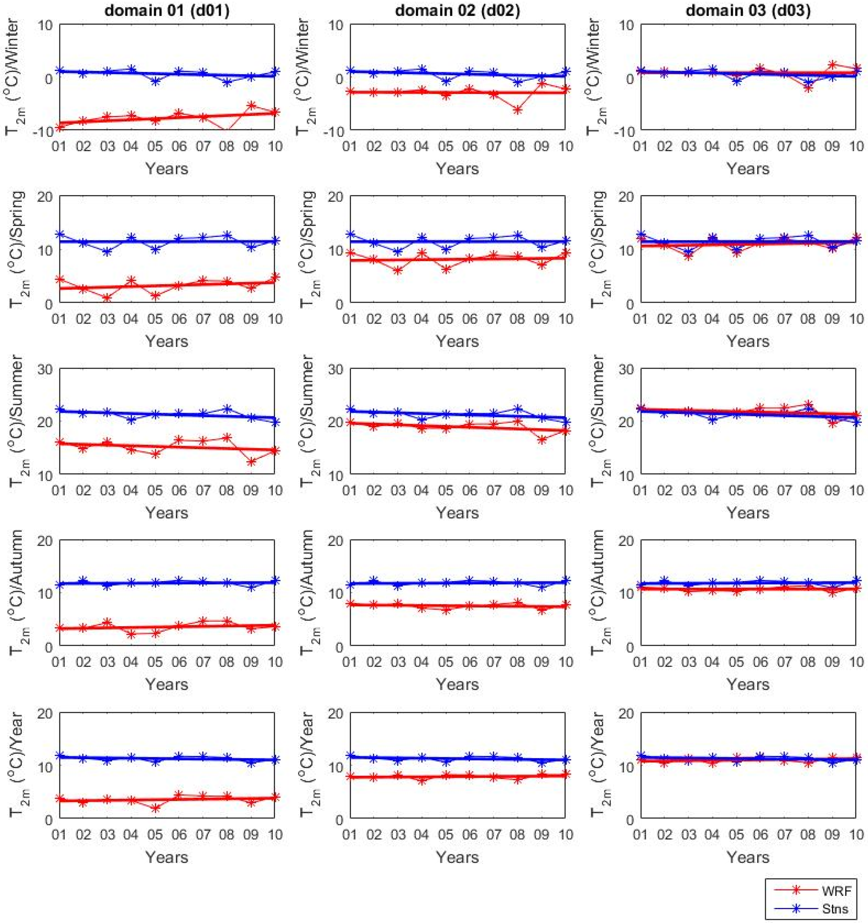
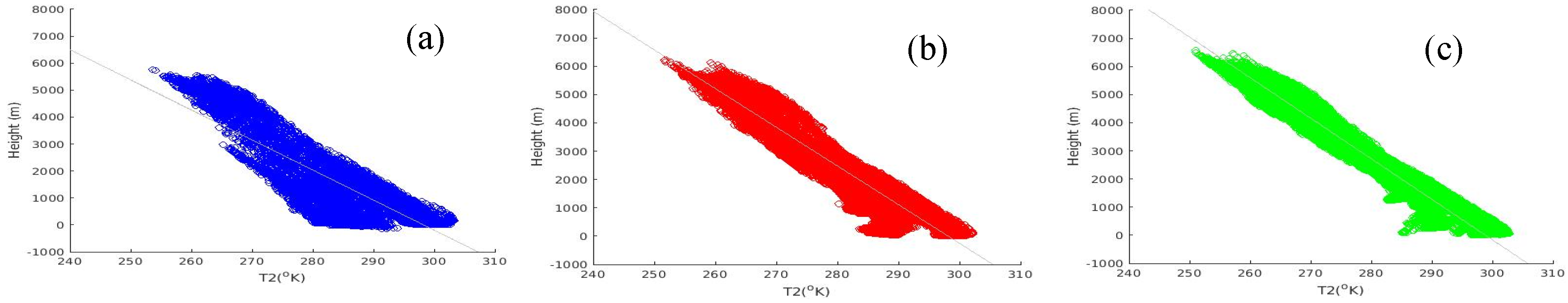
3.2. Station-Averaged Temperature Trends

This section examines the extent to which WRF was accurate in reproducing the spatio-temporal variability of temperature in the three domains. There were only ten stations’ data available for the 10 year time period (i.e., 2001 through 20110). The WRF output was compared with the station data by performing a lapse rate correction to adjust vertically from the WRF grid point elevation to the station elevation, as detailed below (Figure 3). For all three domains, WRF underpredicted the average annual and seasonal temperatures in all seasons. WRF showed a positive correlation with the station data (

Table 5. Mean RMSE (°C), mean bias (°C), and Pearson correlation coefficient (r; unitless) between station-averaged and WRF interpolated lapse rate corrected 2 m air temperature (T2) in d01, d02, and d03.

		d01	d02	d03
Winter (DJF)	RMSE (°C)	8.4	3.6	0.94
	Mean bias (°C)	−8.3	−3.5	0.23
	Pearson correlation coefficient (r)	0.36	0.6	0.6
Spring (MAM)	RMSE (°C)	8.2	3.3	0.69
	Mean bias (°C)	−8.2	−3.3	−0.49
	Pearson correlation coefficient (r)	0.89	0.91	0.91
Summer (JJA)	RMSE (°C)	6.1	2.4	0.84
	Mean bias (°C)	−6.1	−2.3	−0.51
	Pearson correlation coefficient (r)	0.68	0.73	0.73
Autumn (SON)	RMSE (°C)	8.3	4.3	1.2
	Mean bias (°C)	−8.2	−4.3	−1.1
	Pearson correlation coefficient (r)	0.08	0.18	0.53
Annual	RMSE (°C)	7.7	3.4	0.78
	Mean bias (°C)	−7.7	−3.4	−0.24
	Pearson correlation coefficient (r)	0.7	−0.44	−0.4

) in all seasons. However, most of these trends for temperature were not statistically significant. The important feature was how the simulated temperature and bias changed as the resolution increased. The results showed that RMSE and mean bias were noticeably changed from d01 to d03 in all seasons. This showed that WRF tended to underestimate the 2 m air temperature in d01 (annual mean bias of −7.7°C), d02 (annual mean bias of −3.4°C), and d03 (annual mean bias of −0.24°C), respectively.

Figure 4 shows the change in the mean lapse rate with altitude in all three domains. The average lapse rate for d01, d02, and d03 across the simulated period was estimated to be −6.9167, −6.7863, and −6.8111°C/km, respectively. These lapse rates were used to interpolate the simulated temperature time series vertically to the actual heights of the stations. For each station, the difference between the station height and WRF height was computed, multiplied by the average lapse rate, and added to the simulated temperature values (

Table 6. Stations and the interpolated 2 m air temperature (T2) with lapse rate correction at an annual time scale.

Station	Station Elev. (m)	WRF Elev. (m) in d01	WRF Elev. (m) in d02	WRF Elev. (m) in d03	Diff. (d01)	Diff. (d02)	Diff. (d03)	Interpolated T2 (°C) in d01	Interpolated T2 (°C) in d02	Interpolated T2 (°C) in d03
								T2 = T0 − 0.0069167	T2 = T0 − 0.0067863	T2 = T0 − 0.00681
Astore	2168	3824	3705	3500	−1656	−1537	−1332	11.4541	10.43	9.071
Bunji	1372	3454	2638	1634	−2082	−1266	−262	14.4006	8.591	1.784
Chillas	1250	3097	1932	1397	−1847	−682	−147	12.7751	4.628	1.001
Chitral	1497	3469	2767	2507	−1972	−1270	−1010	13.6397	8.619	6.878
Gilgit	1460	3360	2892	1905	−1900	−1432	−445	13.1417	9.718	3.03
Gupis	2156	4034	3862	4317	−1878	−1706	−2161	12.9896	11.58	14.72
Skardu	2317	3971	3106	2493	−1654	−789	−176	11.4402	5.354	1.199
Khunjerab	4707	3971	5015	5040	736	−308	−333	−5.0907	2.09	2.268
Rama	3140	3749	3627	3394	−609	−487	−254	4.21227	3.305	1.73
Rattu	2920	3925	3572	3403	−1005	−652	−483	6.95128	4.425	3.289

). The station-wise comparison of the mean bias (Table 4) showed that most of the temperature simulations were greatly improved from d01 to d03 at all stations. The results showed that Astore, Chillas, Gilgit, and Skardu stations had the lowest bias in d03. However, Bunji, Chitral, and Gupis had the highest bias in d03.

4. Discussion and Conclusions

The WRF model was applied to simulate the spatiotemporal variability of precipitation and temperature over the Indus Basin from 2000 through 2015 using boundary conditions derived from the CFSR reanalysis dataset. We found that most of the precipitation trends in WRF, TRMM, and station precipitation at gauge locations were not statistically significant, which was consistent with Ahmad et al. [48], Khattak et al. [49], and Norris et al. [23].

The critical aspect was how the simulated precipitation amount and bias changed as resolution increased. The precipitation simulations were significantly improved from d01 (36 km) to d03 (4 km). The annual PBIAS between WRF and stations’ data was decreased from d01 (132%) to d03 (23%). These results seemed broadly consistent with the previous studies [14,15,23,50,51], which also showed a positive influence of increasing resolution on precipitation over complex regions. Moreover, the WRF was significantly correlated with TRMM and station data in most of the seasons (except spring season) in all domains. WRF was able to capture the precipitation trends in most of the seasons, but tended to overestimate precipitation in all domains, which may reflect an underestimation of precipitation by the observed datasets as discussed earlier. Many researchers have revealed that the existing observation dataset network including TRMM 3B42V7 underestimates precipitation amounts by 66% to 300% over the UIB [52,53,54]. The gauges in the UIB in Pakistan suffer from undercatch for winter precipitation, especially snowfall (Norris et al. [15]), which could cause a significant amount of wet bias in this season. However, precipitation occurs in the form of rain in spring and summer seasons over this region, which the rain gauges measure more accurately. This contributed to less discrepancy between WRF precipitation and station observations in the summer season. However, the WRF simulations for temperature were much better than those of precipitation. The mean bias was noticeably reduced with the increasing resolution. The WRF model showed an underestimation of 2 m air temperature in all domains and seasons, which was consistent with prior studies [23] over this region.

The higher resolution simulations show a significantly improved representation of the climatic variables. Therefore, the spatial grid spacing resolution of the inner domain (d03) is high enough to capture the orographic effects in this area. Moreover, the results show that both precipitation and temperature output are largely improved with the increase of the resolution.

Some future research possibilities arise from this discussion. One is that an in-depth sensitivity analysis with different physical parameterization schemes (microphysics, LSM, PBL, and cumulus) may be beneficial in this region. In addition, we used the WRF model to simulate the spatiotemporal variability of precipitation and temperature over the Indus Basin from 2000 through 2015 with boundary conditions derived from the Climate Forecast System Reanalysis (CFSR) data. The CFSR data have been shown to capture the trends overall. However, it would be potentially useful to assess the alternative global reanalysis data products (such as ERA-Interim) to derive the boundary conditions over this region. It is possible that some of those alternative global reanalysis datasets may produce even better results. In this study, we have used the station data and TRMM 3B42V7 dataset to validate the WRF output. However, employing multiple gridded datasets such as GPCC, CRU, and MODIS snow cover product to assess the WRF output would be recommended.

Knowing the limitations of GCMs over complex and rugged terrain, regional climate models were the best available tools to simulate climate change. This study did not intend to analyze the climatic processes that influence the precipitation and temperature, but provided an overview of the ability of WRF to simulate spatiotemporal variability of precipitation and temperature over the UIB. These analyses could provide a better understanding of the limitations and reliability of WRF simulations. In addition, this study presented high-resolution climatological datasets, which could be useful for climate change and other hydrological studies in this region.

References

1. Soncini, A.; Bocchiola, D.; Confortola, G.; Bianchi, A.; Rosso, R.; Mayer, C.; Lambrecht, A.; Palazzi, E.; Smiraglia, C.; Diolaiuti, G. Future Hydrological Regimes in the Upper Indus Basin: A Case Study from a High-Altitude Glacierized Catchment. J. Hydrometeorol. 2014, 16, 306–326. [Google Scholar] [CrossRef] [Green Version]
2. Farhan, S.B.; Zhang, Y.; Ma, Y.; Guo, Y.; Ma, N. Hydrological regimes under the conjunction of westerly and monsoon climates: A case investigation in the Astore Basin, Northwestern Himalaya. Clim. Dyn. 2015, 44, 3015–3032. [Google Scholar] [CrossRef]
3. Immerzeel, W.W.; Beek, L.P.H.; Van Bierkens, M.F.P. Climate change will affect the Asian water towers. Science 2010, 328, 1382–1385. [Google Scholar] [CrossRef] [PubMed]
4. Krakauer, N.Y.; Lakhankar, T.; Dars, G.H. Precipitation Trends over the Indus Basin. Climate 2019, 7, 116. [Google Scholar] [CrossRef] [Green Version]
5. Shafique, M.; Faiz, B.; Bacha, A.S.; Ullah, S. Evaluating glacier dynamics using temporal remote sensing images: A case study of hunza valley, northern Pakistan. Environ. Earth Sci. 2018, 77, 162. [Google Scholar] [CrossRef]
6. Hewitt, K. The Karakoram Anomaly? Glacier Expansion and the ‘Elevation Effect’ Karakoram Himalaya. Mt. Res. Dev. 2005, 25, 332–340. [Google Scholar] [CrossRef] [Green Version]
7. Chaudhary, Q.Z.; Mahmood, A.; Rasul, G.; Afzaal, M. Climate Change Indicators of Pakistan; Technical report no. PMD-22/2009; Pakistan Meteorological Department: Islamabad, Pakistan, 2009; pp. 1–43.
8. Mahessar, A.A.; Qureshi, A.L.; Dars, G.H.; Solangi, M.A. Climate change impacts on vulnerable Guddu and Sukkur Barrages in Indus River, Sindh. Sindh Univ. Res. J. 2017, 49, 137–142. [Google Scholar]
9. Eckstein, D.; Künzel, V.; Schäfer, L. Global Climate Risk Index 2018: Who Suffers Most from Extreme Weather Events? Weather-Related Loss Events in 2016 and 1997 to 2016; Germanwatch Nord-Süd Initiative e.V: Bonn, Germany, 2017. [Google Scholar]
10. Immerzeel, W.W.; Bierkens, M.F.P. Asia’s water balance. Nat. Geosci. 2012, 5, 841–842. [Google Scholar] [CrossRef]
11. Amin, A.; Iqbal, J.; Asghar, A.; Ribbe, L. Analysis of current and futurewater demands in the Upper Indus Basin under IPCC climate and socio-economic scenarios using a hydro-economic WEAP Model. Water 2018, 10, 537. [Google Scholar] [CrossRef] [Green Version]
12. Kazmi, D.H.; Li, J.; Rasul, G.; Tong, J.; Ali, G.; Cheema, S.B.; Liu, L.; Gemmer, M.; Fischer, T. Statistical downscaling and future scenario generation of temperatures for Pakistan Region. Theor. Appl. Climatol. 2015, 120, 341–350. [Google Scholar] [CrossRef]
13. Su, B.; Huang, J.; Gemmer, M.; Jian, D.; Tao, H.; Jiang, T.; Zhao, C. Statistical downscaling of CMIP5 multi-model ensemble for projected changes of climate in the Indus River Basin. Atmos. Res. 2016, 178–179, 138–149. [Google Scholar] [CrossRef]
14. Maussion, F.; Scherer, D.; Mölg, T.; Collier, E.; Curio, J.; Finkelnburg, R. Precipitation seasonality and variability over the Tibetan Plateau as resolved by the high Asia reanalysis. J. Clim. 2014, 27, 1910–1927. [Google Scholar] [CrossRef] [Green Version]
15. Norris, J.; Carvalho, L.M.V.; Jones, C.; Cannon, F.; Bookhagen, B.; Palazzi, E.; Tahir, A.A. The spatiotemporal variability of precipitation over the Himalaya: Evaluation of one-year WRF model simulation. Clim. Dyn. 2017, 49, 2179–2204. [Google Scholar] [CrossRef]
16. Scalzitti, J.; Strong, C.; Kochanski, A.K. A 26 year high-resolution dynamical downscaling over the wasatch mountains: Synoptic effects on winter precipitation performance. J. Geophys. Res. 2016, 121, 3224–3240. [Google Scholar] [CrossRef] [Green Version]
17. Scalzitti, J.; Strong, C.; Kochanski, A. Climate change impact on the roles of temperature and precipitation in western US snowpack variability. Geophys. Res. Lett. 2016, 43, 5361–5369. [Google Scholar] [CrossRef]
18. Sikder, S.; Hossain, F. Assesment of the weather research and forecasting model generalized parameterization schemes for advancement of precipitation forecasting in monsoon-driven river basins. J. Adv. Model. Earth Syst. 2016, 8, 1210–1228. [Google Scholar] [CrossRef] [Green Version]
19. Collier, E.; Immerzeel, W.W. High-resolution modeling of atmospheric dynamics in the Nepalese Himalaya. J. Geophys. Res. Atmos. 2015, 120, 9882–9896. [Google Scholar] [CrossRef]
20. Sato, T. Mechanism of orographic precipitation around the meghalaya plateau associated with intraseasonal oscillation and the diurnal cycle. Mon. Weather Rev. 2013, 141, 2451–2466. [Google Scholar] [CrossRef] [Green Version]
21. Maussion, F.; Scherer, D.; Finkelnburg, R.; Richters, J.; Yang, W.; Yao, T. WRF simulation of a precipitation event over the Tibetan Plateau, China - An assessment using remote sensing and ground observations. Hydrol. Earth Syst. Sci. 2011, 15, 1795–1817. [Google Scholar] [CrossRef] [Green Version]
22. Li, M.; Ma, Y.; Hu, Z.; Ishikawa, H.; Oku, Y. Snow distribution over the Namco lake area of the Tibetan Plateau. Hydrol. Earth Syst. Sci. 2009, 13, 2023–2030. [Google Scholar] [CrossRef] [Green Version]
23. Norris, J.; Carvalho, L.M.V.; Jones, C.; Cannon, F. Deciphering the contrasting climatic trends between the central Himalaya and Karakoram with 36 years of WRF simulations. Clim. Dyn. 2018, 52, 159–180. [Google Scholar] [CrossRef]
24. Viterbo, F.; von Hardenberg, J.; Provenzale, A.; Molini, L.; Parodi, A.; Sy, O.O.; Tanelli, S. High-Resolution Simulations of the 2010 Pakistan Flood Event: Sensitivity to Parameterizations and Initialization Time. J. Hydrometeorol. 2016, 17, 1147–1167. [Google Scholar] [CrossRef]
25. Gao, Y.; Xu, J.; Chen, D. Evaluation of WRF mesoscale climate simulations over the Tibetan Plateau during 1979-2011. J. Clim. 2015, 28, 2823–2841. [Google Scholar] [CrossRef] [Green Version]
26. Skamarock, W.C.; Klemp, J.B.; Dudhia, J.; Gill, D.O.; Barker, D.M.; Duda, M.G.; Huang, X.-Y.; Wang, W.; Powers, J.G. A Description of the Advanced Research WRF Version 3; NCAR Technical Note NCAR/TN-475+STR; NCAR: Boulder, CO, USA, 2008. [Google Scholar]
27. Saha, S.; Moorthi, S.; Pan, H.L.; Wu, X.; Wang, J.; Nadiga, S.; Tripp, P.; Kistler, R.; Woollen, J.; Behringer, D.; et al. The NCEP climate forecast system reanalysis. Bull. Am. Meteorol. Soc. 2010, 91, 1015–1057. [Google Scholar] [CrossRef]
28. Dimri, A.P.; Niyogi, D.; Barros, A.P.; Ridley, J.; Mohanty, U.C.; Yasunari, T.; Sikka, D.R. Western Disturbances: A review. Rev. Geophys. 2015, 53, 225–246. [Google Scholar] [CrossRef]
29. Jamro, S.; Dars, G.H.; Ansari, K.; Krakauer, N.Y. Spatio-Temporal Variability of Drought in Pakistan Using Standardized Precipitation Evapotranspiration Index. Appl. Sci. 2019, 9, 4588. [Google Scholar] [CrossRef] [Green Version]
30. Frenken, K. Irrigation in Southern and Eastern Asia in Figures: Aquastat Survey—2011; Technical Report; Food and Agriculture Organization (FAO): Rome, Italy, 2012. [Google Scholar]
31. Naz, F.; Dars, G.H.; Ansari, K.; Jamro, S.; Krakauer, N.Y. Drought Trends in Balochistan. Water 2020, 12, 470. [Google Scholar] [CrossRef] [Green Version]
32. Hewitt, K. Glaciers of the Karakoram Himalaya: Glacial Environments, Processes, Hazards and Resources; Springer: Berlin, Germany, 2014. [Google Scholar]
33. Pritchard, D.M.W.; Forsythe, N.; Fowler, H.J.; O’Donnell, G.M.; Li, X.F. Evaluation of upper indus near-surface climate representation by WRF in the High Asia Refined Analysis. J. Hydrometeorol. 2019, 20, 467–487. [Google Scholar] [CrossRef]
34. Bao, X.; Zhang, F. Evaluation of NCEP-CFSR, NCEP-NCAR, ERA-Interim, and ERA-40 reanalysis datasets against independent sounding observations over the Tibetan Plateau. J. Clim. 2013, 26, 206–214. [Google Scholar] [CrossRef] [Green Version]
35. Niu, G.-Y.; Yang, Z.-L.; Mitchell, K.E.; Chen, F.; Ek, M.B.; Barlage, M.; Kumar, A.; Manning, K.; Niyogi, D.; Rosero, E.; et al. The community Noah land surface model with multiparameterization options (Noah-MP): 1 Model description and evaluation with local-scale measurements. J. Geophys. Res. 2011, 116, 1–19. [Google Scholar] [CrossRef] [Green Version]
36. Hong, S.-Y.; Noh, Y.; Dudhia, J. A new vertical diffusion package with an explicit treatment of entrainment processes. Mon. Weather Rev. 2006, 134, 2318–2341. [Google Scholar] [CrossRef] [Green Version]
37. Thompson, G.; Field, P.R.; Rasmussen, R.M.; Hall, W.D. Explicit Forecasts of Winter Precipitation Using an Improved Bulk Microphysics Scheme. Part II: Implementation of a New Snow Parameterization. Mon. Weather Rev. 2008, 136, 5095–5115. [Google Scholar] [CrossRef]
38. Iacono, M.J.; Delamere, J.S.; Mlawer, E.J.; Shephard, M.W.; Clough, S.A.; Collins, W.D. Radiative forcing by long-lived greenhouse gases: Calculations with the AER radiative transfer models. J. Geophys. Res. Atmos. 2008, 113, 2–9. [Google Scholar] [CrossRef]
39. Dudhia, J. Numerical Study of Convection Observed during the Winter Monsoon Experiment Using a Mesoscale Two-Dimensional Model. J. Atmos. Sci. 1989, 46, 3077–3107. [Google Scholar] [CrossRef]
40. Monin, A.S.; Obukhov, A.M. Basic laws of turbulent mixing in the surface layer of the atmosphere. Contrib. Geophys. Inst. Acad. Sci. USSR 1954, 151, e187. [Google Scholar]
41. Kain, J.S. The Kain—Fritsch convective parameterization: An update. J. Appl. Meteorol. 2004, 43, 170–181. [Google Scholar] [CrossRef] [Green Version]
42. Huffman, G.J.; Bolvin, D.T.; Nelkin, E.J.; Wolff, D.B.; Adler, R.F.; Gu, G.; Hong, Y.; Bowman, K.P.; Stocker, E.F. The TRMM Multisatellite Precipitation Analysis (TMPA): Quasi-Global, Multiyear, Combined-Sensor Precipitation Estimates at Fine Scales. J. Hydrometeorol. 2007, 8, 38–55. [Google Scholar] [CrossRef]
43. Ali, A.F.; Xiao, C.; Anjum, M.N.; Adnan, M.; Nawaz, Z.; Ijaz, M.W.; Sajid, M.; Farid, H.U. Evaluation and comparison of TRMM multi-satellite precipitation products with reference to rain gauge observations in Hunza River basin, Karakoram Range, northern Pakistan. Sustainability 2017, 9, 1954. [Google Scholar] [CrossRef] [Green Version]
44. Mann, H.B. Nonparametric tests against trend. Econom. J. Econom. Soc. 1945, 13, 245–259. [Google Scholar] [CrossRef]
45. Kendall, M.G. Rank Correlation Methods; Griffin: London, UK, 1948. [Google Scholar]
46. Arfan, M.; Lund, J.; Hassan, D.; Saleem, M.; Ahmad, A. Assessment of spatial and temporal flow variability of the Indus River. Resources 2019, 8, 103. [Google Scholar] [CrossRef] [Green Version]
47. Hu, M.; Sayaman, T.; TRY, S.; Takara, K.; Tanaka, K. Trend analysis of hydro-climatic variables in the Kamo River Basin, Japan. Water 2019, 11, 1782. [Google Scholar] [CrossRef] [Green Version]
48. Ahmad, I.; Tang, D.; Wang, T.; Wang, M.; Wagan, B. Precipitation trends over time using Mann-Kendall and spearman’s Rho tests in swat river basin, Pakistan. Adv. Meteorol. 2015, 2015. [Google Scholar] [CrossRef] [Green Version]
49. Khattak, M.S.; Babel, M.S.; Sharif, M. Hydro-meteorological trends in the upper Indus River basin in Pakistan. Clim. Res. 2011, 46, 103–119. [Google Scholar] [CrossRef]
50. Heikkilä, U.; Sandvik, A.; Sorteberg, A. Dynamical downscaling of ERA-40 in complex terrain using the WRF regional climate model. Clim. Dyn. 2011, 37, 1551–1564. [Google Scholar] [CrossRef] [Green Version]
51. Caldwell, P.; Chin, H.N.S.; Bader, D.C.; Bala, G. Evaluation of a WRF dynamical downscaling simulation over California. Clim. Chang. 2009, 95, 499–521. [Google Scholar] [CrossRef] [Green Version]
52. Khan, A.J.; Koch, M. Correction and informed regionalization of precipitation data in a high mountainous region (Upper Indus Basin) and its effect on SWAT-modelled discharge. Water 2018, 10, 1557. [Google Scholar] [CrossRef] [Green Version]
53. Khan, A.J.; Koch, M.; Chinchilla, K.M. Evaluation of Gridded Multi-Satellite Precipitation Estimation (TRMM-3B42-V7) Performance in the Upper Indus Basin (UIB). Climate 2018, 6, 76. [Google Scholar] [CrossRef] [Green Version]
54. Palazzi, E.; Von Hardenberg, J.; Provenzale, A. Precipitation in the Hindu-Kush Karakoram Himalaya: Observations and future scenarios. J. Geophys. Res. Atmos. 2013, 118, 85–100. [Google Scholar] [CrossRef]
Figure 1. Configuration of the WRF model domain and topography. The study has three nested domains (d01–d03) with horizontal resolutions increasing inward from 36 km to 12 km to 4 km grid cell resolution, respectively. The elevation of the study region was derived from a 90 m resolution SRTM DEM.
Applsci 10 01765 g001
Figure 2. Time series comparisons between WRF (red), TRMM (green), and the mean of stations (“observed”; blue) for Domain 01 (d01; left column), Domain 02 (d02; middle column), and Domain 03 (d03; right column). From top to bottom, the five rows correspond to winter (DJF), spring (MAM), summer (JJA), autumn (SON), and annual. The straight lines are least-squares linear regressions.
Applsci 10 01765 g002
Figure 3. Time series comparisons of temperature (T2) between WRF (red) and the mean of stations (“Observed”; blue) in d01 (left column), d02 (middle column), and d03 (right column) with lapse rate correction. From top to bottom, the five rows correspond to winter (DJF), spring (MAM), summer (JJA), autumn (SON), and annual. The straight lines are least-squares linear regressions.
Applsci 10 01765 g003
Figure 4. Lapse rate between T2 (Kelvin) and height (m) in d01 (a), d02 (b), and d03 (c).
Applsci 10 01765 g004