Eco-Efficiency Assessment for Some European Countries Using Slacks-Based Measure Data Envelopment Analysis

Abstract

One problem raised by the lack of energy efficiency is the generation of more greenhouse gases (GHGs) that can cause air pollution and climate change. Ecological efficiency (eco-efficiency) means the efficiency of resources used. A poor performance from this efficiency can then be detected for further improvement. In this research, we conduct an assessment on the eco-efficiency for some European countries as they consume a large part of global energy annually. A total of 17 European countries were selected as decision making units (DMUs) and assessed by the Slacks-based measure (SBM) Data Envelopment Analysis (DEA) model. Indices including Catch-Up, Frontier-Shift, and Malmquist Productivity Index (MPI) have been used to evaluate eco-efficiency, as well as efficiency change, technological change, and productivity change, over 2013–2017. In the model, energy consumption and share of renewable energy are used as energy inputs, and labor productivity and gross capital formation are used as economy inputs. On the other hand, GDP is used as a desired output, and CO₂ emissions is used as one undesired output. The experimental results show that the 17 countries as a whole lacked eco-efficiency in 2013–2017, implying more efforts are required to improve their eco-efficiency.

1. Introduction

1.1. Backround

In the past few decades, many countries have been devoted to developing their economies. One of the adverse effects of economic activities is the degradation to our environment [1]. Recently, ecological efficiency (eco-efficiency) has been highly valued as it can help transform unsustainable development into sustainable development [2]. The term “eco-efficiency” was coined by the World Business Council for Sustainable Development (WBCSD) in its 1992 publication “Changing Course” and at the 1992 Earth Summit as well. Eco-efficiency emphasizes the importance of better use of resources so that more goods and services can be generated from the same level of (or fewer) inputs. Eco-efficiency also means the creation of less waste and pollution. In the private sector, eco-efficiency can be a means for companies to implement Agenda 21, a term that has become synonymous with a management philosophy geared toward sustainability that combines ecological and economic efficiency [3].

Eco-efficiency is measurable based on selected input and output variables. For example, the authors of reference [2] measured the co-efficiency as the ratio between the value of what has been produced (e.g., GDP) and the environment impacts of the product or service (e.g., SO₂ emissions). The purpose of eco-efficiency measurement is to best utilize inputs such as energy, water, soil, and raw materials so as to maximize the benefit to human beings [4] or minimize bad outputs such as pollution and CO₂, which can damage our environment. For every country in the world, improving eco-efficiency is necessary, as the protection of the environment is everyone’s responsibility.

1.2. Problem Definition

One problem raised by the lack of eco-efficiency is the generation of more greenhouse gases (GHGs), which can further lead to the global warming effect. The global warming effect, in turn, can lead to climate change, which might result in disasters and threaten the lives of human beings. International organizations have developed some programs to deal with the global warming effect. For example, the Paris Agreement initiated at the COP21 meeting held in December 2015 has set an objective to keep the rise in average global temperature below 2 °C [5]. The achievement of this difficult objective requires collective efforts from all countries. To achieve this objective, eco-efficiency is considered one of the effective approaches [6,7]. This is why the assessment of eco-efficiency has become the focus of this research. Though every country in the world needs to improve eco-efficiency, in this research, we focused on European countries, as they consume a lot of global energy annually. In fact, energy consumption, especially the use of fossil fuels, is one of the main sources of GHGs. As many European countries require the import of energy sources, they spend a large amount of money on energy and are vulnerable to energy shortages. A higher eco-efficiency means a lower energy cost and a lower possibility of energy shortage. In the past, based on the principles of a “recirculating economy,” European countries have developed advanced and sustainable models for production and consumption [8]. The implementation of the circular economy is one of the priorities of the European Union, and energy efficiency is one of its pillars [9]. However, the recent eco-efficiency of European countries is unclear, as the information reported in many past studies is outdated. In addition, the year-on-year improvement or decrease in eco-efficiency for European countries have rarely been revealed. This lack of information leads to the difficulty in updating environment policy in order to approach the objective set in the Paris Agreement.

1.3. Objectives

The objectives of this research include (1) to provide eco-efficiency assessment for some European countries for the period of 2013–2017, so that these counties can understand their recent performance on this efficiency; (2) to understand the improvement or decrease in efficiency of a country over a specified period of time; and (3) to find some policy implications.

In this research, a total of 17 European countries were selected as Decision Making Units (DMUs) and evaluated using the Slacks-based measure (SBM) Data Envelopment Analysis (DEA) together with the Malmquist Index (MI). The DEA component is used to measure the relative efficiency of the DMUs, while the MI component measures the improvement or decrease in efficiency of a DMU over a specific period of time [10]. This approach can help us to achieve the first and second objectives. In the SBM DEA model, energy consumption per capita and share of renewable energy in total energy consumption are used as energy inputs, while labor productivity and gross capital formation are used as economy inputs. In terms of output, Gross Domestic Product (GDP) per capita is used as one desired output, and CO₂ emissions per capita is used as one undesired output. For change analysis, we employ Catch-Up and Frontier-Shift and Malmquist productivity index (MPI) to assess the efficiency change, technological change, and total productivity change, respectively for these DMUs. The results are helpful for these countries to understand their current performance.

The rest of this paper is organized as follows: Section 2 includes a literature review on DEA and relevant research; Section 3 details the methodology; Section 4 details data collection and verification; Section 5 specifies experimental results; and Section 6 gives conclusions and future research directions.

2. Literature Review

2.1. DEA Introduction

Based on Farrell [11], in which an efficiency concept was introduced with one single information and one yield, DEA was introduced by Charnes et al. (1978) [12]. It is a linear programming method that can be used to assess the relative efficiency of DMUs. Through identifying a subset of efficient “best practice” DMUs, the DMU can construct a frontier and determine the relative efficiency for the remaining DMUs by measuring their distance from this frontier. The DEA model proposed by Charenes et al. [12] is termed the CCR model in homage to those authors. The DEA model was advanced to include numerous sources of information and various yields for a DMU under the prerequisite of constant returns to scale (CRS). In a later study [13], this prerequisite was relaxed, and the DEA advanced to incorporate variable returns to scale (VRS). This DEA model is termed the BCC model.

DEA is a kind of non-parametric methodology, which calculates frontier directly from the observations of DMUs. DEA has likewise been utilized to provide new comprehension of exercises (substances) that do not have comparative units in information sources and yields [14]. For applications, DEA has been used in various areas such as banking, agriculture, medicinal services, transportation, assembling, and administration [15].

The conventional DEA assumes an isotonocity property for variables. The isotonocity property means that the increase of input may reduce the efficiency, while the increase of output may increase efficiency [16]. However, this assumption is not suitable for some cases. For example, the increase of undesired outputs such as pollutants will decrease efficiency. Therefore, DEA has been advanced to handle undesired output. Reference [17] included a concise review and gave a detailed structure of DEA efficiency measurement with undesired output. Based on Ramli and Munisamy [18], Figure 1 gives a structure of approaches available for DEA efficiency measurement with undesired output. For more details, please refer to reference [17].

DEA efficiency measurements with undesired output can be classified into the two main kinds: indirect and direct approaches [18].

The indirect approaches transform the data of the undesired output to become the desired output [17]. As the indirect approaches manipulate the undesired output value, they can be included in the standard DEA model with the desired output. Methods including “additive inverse,” “undesirable output as input,” and “translation invariance” are belonging to the indirect approaches. They are introduced as follows. The “additive inverse method” transforms the undesired output by multiplying its value by −1 [19]. The “undesirable output as input method” considers undesired outputs as inputs. The undesired outputs variables are moved from the output side to the input side of the DEA model [20]. However, such treatment does not conform to physical laws and standard production theory as it incurs conceptual confusion and does not reflect the true production process in the DEA result [21]. The “translation invariance method” adds a large scalar to each of the undesired output values to make the resulting output positive [22]. However, one drawback of this approach is that the scalar selected can change the efficient frontier and shift the position of zero. The authors of reference [18] suggested the incorporation of undesired outputs with desired outputs by giving a negative sign to an undesired output. However, the efficiency scores and ranking obtained for the variables from this kind of “non-separating” outputs approach are different from those obtained from those with separation on the outputs. This approach is applicable in cases were there is only one negative output (or undesired output).

The direct approach uses undesired output data directly to treat undesired outputs appropriately [17]. They include the Hyperbolic Efficiency (HE) model, the Slack-Based Measure (SBM) model, and the Directional Distance Function (DDF) model. The HE model modifies multilateral productivity with the HE measure, in which desired and undesired outputs are treated differently [23]. This approach focuses on increasing the desired output that is strongly disposable (i.e., the waste can be released without cost) and decreasing undesired output that is weakly disposable (i.e., the waste needs to be released with cost). However, this approach is complicated when finding a solution due to being non-linear programming. The original Slack-based measure (SBM) DEA model can be extended to include undesired output. For example, Zhou et al. [24] extended the original slack-based measure (SBM) model, proposed by Tone [25], to include undesired output. This model minimizes the ratio of the average undesired output reduction to the average desired output increment. In that model, slack values of inputs as well as desired outputs and undesired outputs were used to compute a linear combination of DMUs. This non-radial model was employed to assess economic and environmental performance. Compared with a radial model, a non-radial model provides a higher discriminating power in modeling environmental performance [24]. Directional Distance Function (DDF) model is a direct approach that can be extended to include desired outputs and reduce undesired outputs simultaneously based on a given direction vector [26]. However, one major drawback of this model is that the direction vector to the production boundary is fixed arbitrarily, thus it may not provide the best efficiency measures. Due to the drawbacks mentioned above, combined models of DEA approach have been proposed. These include Portela et al. [27] proposed the range directional model, Fukuyama and Weber [28] proposed the directional network slack–based inefficiency model, and Färe and Grosskopf [29] proposed the slacks-based measure model based on directional distance function.

2.2. Relevant Researches

DEA-based approaches have been widely used for performance assessment, including eco-efficiency. Choi et al. [30] used SBM DEA to assess the CO₂ emission of some regions in China. The results showed that the east region had preferred CO₂ emanation efficiency, though the west region had the least CO₂ discharge proficiency. The results can help the Chinese government to characterize its natural resource strategies. Lee et al. [31] employed SBM-DEA to survey the natural efficiency of port urban communities. In that study, work populace was used as one input variable. On the other hand, gross territorial local item and holder throughput were used as the desirable outputs, while nitrogen oxide (NOx), sulfur oxide (SO₂), and carbon dioxide (CO₂) outflows were used as undesired outputs. The results showed that Singapore, Busan, Rotterdam, Kaohsiung, Antwerp, and New York had the best efficiency, while Tianjin had the worst ecologically productivity. Camioto et al. [32] used SBM DEA to investigate vitality efficiency of BRICs countries (Brazil, Russia, India, China), South Africa, and G7 countries (Canada, France, Germany, Italy, Japan, the United Kingdom, and the United States). In that study workforce, net fixed capital development and energy utilization were used as inputs, while CO₂ and GDP were used as outputs. The results showed that the BRICs countries have different vitality substances, which will likewise result in various vitality arrangements. In contrast, the G7 countries are more homogeneous. Reference [33] proposed a hybrid approach combining the Analytical Hierarchical Process (AHP) and the Data Envelopment Analysis (DEA) methodologies to deal with the decision-making problem of choosing the best of several alternatives. The comparison among them is based on both qualitative and quantitative criteria. This method is capable of dealing with a situation where more than one alternative turns out to be efficient.

Other studies also contribute to eco-efficiency assessment. Bian et al. [34] developed several DEA models to assess efficiency of resource and environment for some DMUs. However, due to different results obtained from these models, the selection of the right model for application becomes difficult. To resolve this difficulty, the authors proposed an extended Shannon-DEA procedure to find a suitable model. Then, the data collected from 30 provinces in China were used for an empirical study. Alves et al. [35] applied the DEA model to evaluate the efficiency of resources and the environment for some European countries in the two time periods—2000–2004 and 2005–2011. In that study, capital, labor, fossil fuels, and renewable energy consumption were used as input variables, while GDP and GHG were used as output variables. The results showed that these European countries had improved eco-efficiency in the time period 2005–2011. Moutinho et al. [36] used a hybrid approach combining the DEA model with the quantum regression technique to assess the economic and environmental efficiency for European countries in 2001–2012. First, DEA was used to measure the performance of the countries, and then the quantum regression technique was used to identify different efficiency points among the countries. In that study, labor productivity, capital productivity, weight of fossil energy, and share of renewable energy in GDP were used as input variables, while GDP and GHGs were used as output variables. The results showed that GHG emissions is significantly affected by the shares of renewable energy and non-renewable energy used. Taxation can also affect the rankings of technical eco-efficiency. Moutinho et al. [37] used a DEA model combined with a Tapio decoupling model to assess the eco-efficiency of Latin American nations. First, the DEA was used to assess the efficiency changes of eco-efficiency for these countries, and then the Tapio decoupling model was used to show the decoupling index elasticity. That study used labor productivity, gross capital formation productivity, energy use, and renewable energy consumption as inputs and proportion of the GDP and CO₂ emission as outputs. Halkos et al. [38] used a DEA model to evaluate the efficiency of the 28 EU countries in years 2008, 2010, 2012, and 2014. That study considered the following eight factors, metropolitan strong waste (MSW), age, work rate, capital arrangement, total domestic output (GDP), populace thickness, and out of the blue sulfur oxide (SOx), nitrogen oxide (NOx), and ozone depleting substances (GHG) emanations from waste for the pertinent nations. Wang et al. [39] proposed a DEA model combined with a global benchmark technology to estimate the regional eco-efficiency in China in 2003–2014. That study used capital stock, labor, construction land area, water consumption, and energy consumption as inputs and GDP, solid waste emission, household refuse, SO₂ emissions, soot and industrial dust emission, and waste-water emissions as outputs. The experimental results showed that resource consumption and environmental efficiency have not been best utilized. The eastern region is the best, while the northwest region is the worst in terms of ecological efficiency. This trend is expected to continue. They concluded that scientific and technical progress and management play a main role in improving ecological efficiency in China. However, as the above-mentioned studies are dated, current research for updating the status for different countries in different areas is necessary.

3. Methodology

In this research, the SBM DEA model is used to assess the eco-efficiency of DMUs, and the Malmquist Productivity Index (MPI) is used to analyze the efficiency change, technological change, and total productivity change for DMUs. The SBM DEA and MPI are detailed in Section 3.1 and Section 3.2, respectively.

3.1. Slack-Based Measure (SBM) DEA Model

DEA is a kind of non-parametric analysis tool that can be used to assess the relative efficiency of entities, termed as decision-making units (DMUs). A DMU is considered to be efficient if it can produce more outputs with the same or fewer number of inputs. However, a conventional DEA model does not consider undesirable outputs such as air pollution and hazardous materials. Thus, the conventional DEA model cannot be used in this present research because undesirable outputs will be included.

The Slacks-based measure (SBM) DEA model proposed in Tone [25] was found to be unable to deal with undesirable outputs [40]. The SBM DEA is a kind of non-radial and non-oriented model that uses input and output slacks to measure efficiency directly. To deal with undesirable outputs, the SBM DEA was modified in reference [41], and two variants of SBM DEA, i.e., Bad-Output and Non-Separable models, were proposed. The Bad-Output model deals with good (desirable) and bad (unwanted) outputs independently, whereas the Non-Separable model assumes that connection exists between good inputs and bad outputs. The Non-Separable model assumes that reducing unwanted outputs will reduce desirable output due to their connection. In this research, the Bad-Output model is used as there is no connection between desirable outputs and undesirable outputs.

In reference [41], each DMU in the SBM is assumed to have the three factors—inputs, good (desirable) outputs, and bad (undesirable) outputs. The three factors are represented by the three vectors x $\in$ $R^m$, $Y^g\in R^{s1}$, and $Y^b\in R^{s2}$, respectively.

A DMU can be represented as $\left(x_o,y_o^g,y_o^b\right)$ and evaluated by two kinds of output (desirable and undesirable), where $y_o^g$ denotes the desirable output and $y_o^b$ denotes the undesirable output. The production possibility set P is defined as follows.

$$\mathrm{P}=\left\{\left(x,y^g,y^b\right)\left| x \ge X\lambda , y^g \le Y^{g }\lambda , y^b \ge Y^b\lambda , L \le e\lambda \le U, \lambda \ge 0\right|\right\}$$

where λ is the intensity vector and L and U are the lower and upper bounds of the intensity vector, respectively.

A DMU $\left(x_o,y_o^g,y_o^b\right)$ is efficient if there is a vector $\left(x_o,y_o^g,y_o^b\right)$ $\in$ P such that $x_0\ge x, y_o^g\le y^g, y_o^b\ge y^b$ with at least one strict inequality. The SBM proposed by Tone [25] is then modified in Equation (1).

$$[SBM]{\rho }^{*}=min\frac{1-\frac{1}{m}{{\displaystyle \sum }}_{i=1}^m \frac{s_{io}^{-}}{x_{io}}}{1+\frac{1}{s}\left({{\displaystyle \sum }}_{r=1}^{s_1} \frac{S_r^g}{y_{ro}^g }+ {{\displaystyle \sum }}_{r=1}^{s_2} \frac{S_r^b}{y_{ro}^b}\right)}$$

(1)

subject to

$$\begin{gathered} x_o=X\lambda +S^{-} \\ {y}_o^g=Y\lambda -S^g \\ {y}_o^b=Y\lambda +S^b \\ L\le e\lambda \le U \\ {S}^{-},S^g,S^b,\lambda \ge 0. \end{gathered}$$

The vectors $S^{-}$ and $S^b$ refer to the excesses in inputs and undesirable outputs, and $S^g$ represents the shortage in desirable outputs. The $DM{U}_o$ is efficient with consideration of bad output if and only if ρ* = 1 or in the other words, $S^{-*}$= 0, $S^{g*}$= 0 and $S^{b*}$= 0.

3.2. Malmquist Productivity Index (MPI)

The Malmquist Productivity Index (MPI) [42] was developed to measure the changes in technological productivity and the improvement. To measure the change in technological productivity, several other indexes were introduced. An explanation of the method can be found in reference [10]. Equation (2) shows the output-based MPI defined in Walter et al. [41].

$$MPI={\left[\frac{d_o^s\left(x_t,y_t\right)}{d_o^s\left(x_s,y_s\right)}\times \frac{d_o^t\left(x_t,y_t\right)}{d_o^t\left(x_s,y_s\right)}\right]}^{1/2}$$

(2)

where $d_o^s$ is a distance function measuring the efficiency of conversion of inputs x_s to outputs y_s in the period s. DEA efficiency is considered a distance measure because it reflects the efficiency of converting inputs to outputs. If there is a technological change in period t, then,

$$d_o^t\left(x_s,y_s\right)=\mathrm{Efficiency}\mathrm{of}\mathrm{conversion}\mathrm{of}\mathrm{input}\mathrm{in}\mathrm{period}\mathrm{s}\mathrm{to}\mathrm{output}\mathrm{in}\mathrm{period}s\ne d_o^s\left(x_s,y_s\right)$$

MPI is defined as a geometric average of the efficiency change and technological change in the two periods s and t. According to Färe et al. (1994) [43], the MPI in Equation (2) can be written as Equation (3).

$$MPI=\frac{d_o^t\left(x_t,y_t\right)}{d_o^s\left(x_s,y_s\right)}{\left[\frac{d_o^s\left(x_s,y_s\right)}{d_o^t\left(x_s,y_s\right)}\times \frac{d_o^s\left(x_t,y_t\right)}{d_o^s\left(x_t,y_t\right)}\right]}^{1/2}=\mathrm{Efficiency}\mathrm{change}\times \mathrm{Technical}\mathrm{change}$$

(3)

MPI can be used to measure overall productivity of DMU over time. If MPI > 1, it indicates productivity improvement for the DMU; if MPI = 1, it indicates no productivity change; and if MPI < 1, it means productivity recession. As MPI productivity change is a multiplicative composite of efficiency and technological changes, the change in productivity comes from either an efficiency change, a technological change, or both.

3.3. Efficiency Change or Catch-Up Effect

In Equation (3), the first clause is defined as “efficiency change” or “catch-up effect,” which is a value indicating the degree and direction of efficiency change of a DMU. An efficiency change value > 1 means a relative improved efficiency from the period s to t; an efficiency change value = 1 means no change; an efficiency change value < 1 means efficiency recession.

3.4. Technological Change or Frontier-Shift Effect

In Equation (3), the second clause is defined as “technological change” or “frontier-shift effect” (or innovation effect), which is a value indicating the degree and direction of frontier shift from the time periods s to t. If the technological change value > 1, it indicates technological progression; when the technological change value = 1, it means no change; and if the technological change value < 1, it indicates technological regression.

4. Data Collection and Correlation Analysis

Section 4.1 details the selection of DMUs; Section 4.2 specifies the selection of input and output variables; finally, Section 4.3 details the correlation check for the input and output variables selected in this research.

4.1. Selection of DMUs

In this research, 17 European countries were selected as DMUs.

Table 1. List of 17 selected countries (decision-making units—DMUs).

DMU	Country	DMU	Country	DMU	Country
1	Austria	7	Greece	13	Portugal
2	Belgium	8	Hungary	14	Spain
3	Czech Republic	9	Italy	15	Sweden
4	Finland	10	Netherlands	16	Switzerland
5	France	11	Norway	17	United Kingdom
6	Germany	12	Poland

shows the list of 17 DMUs to be investigated in this research. They include Austria, Belgium, the Czech Republic, Finland, France, Germany, Greece, Hungary, Italy, the The Netherlands, Norway, Poland, Portugal, Spain, Sweden, the United Kingdom, and Switzerland. In DEA, these countries are termed DMUs, and each has been assigned a DMU code.

4.2. Selection of Variables

For SBM DEA, the selection of input and output variables is necessary before assessing DMUs. After reviewing previous research as shown in

Table 2. Summary of input and output variables used in previous studies.

Research Title	Input Variable	Output Variable
Lee et al. [31]	− Work populace	− Gross territorial local item (D) − Holder throughput (D) − Nitrogen oxide (NOx) (UD) − Sulfur oxide (SO2) (UD) − Carbon dioxide (CO2) (UD)
Alves et al. [35]	− Capital − Labor − Fossil fuels − Renewable Energy consumption	− GHG − GDP
Moutinho et al. [36]	− Labor productivity − Capital productivity − Weight of fossil energy − Share of renewable energy in GDP	− GDP − GHG
Moutinho et al. [37]	− Labor productivity − Gross capital formation productivity − Energy use − Renewable energy consumption	− GDP − CO2 emission
Halkos et al. [38]	− Metropolitan strong waste (MSW) − Age − Work rate	− Capital arrangement − GDP − Populace thickness − Blue sulfur oxide (SOx) − Nitrogen oxide (NOx) − GHG
Wang et al. [39]	− Capital stock − Labor − Construction land area − Water consumption − Energy consumption	− GDP − Solid waste − Household refuse − SO2 emission − Soot − Industrial dust − Waste water

D: desired output; UD: undesired output.

, we use two kinds of input variables: energy input and environmental input. Factors including energy consumption and share of renewable energy were used as energy inputs while variables while factors including labor productivity and capital stock were used as environmental input variables. However, as the as the data of the factor capital stock is not available, thus we use the gross capital formation productivity instead. In this research, the factor gross domestic product (GDP) is used as a desired output, while CO₂ emissions is used as an undesired output.

Table 3. Input and output variables and unit of measurement.

Variable	Code	Variable	Unit of Measurement
Input	X1	Energy consumption	Ton of oil equivalent per capita
	X2	Labor productivity	GDP per employer (USD)
	X3	Share of renewable energy in total energy consumption	Percentage (%)
	X4	Gross Capital Formation productivity	Percentage GDP (%)
Output	Y1	GDP per capita	USD
	Y2	CO2 emissions per capita	Metrics tons per capita

lists all the input and output variables and their units of measurement.

The measurements of these variables are detailed as follows. The energy consumption is measured by ton of oil equivalent per capita and was collected from the World Bank [44]. Labor productivity is calculated as total GDP per total labor force employed, and all related figures for calculation are provided by the World Bank. The share of renewable energy in total final energy consumption is computed as total renewable consumption per total final energy consumption. Renewable consumption is collected from Eurostat, and total energy consumption is collected from the Enerdata Yearbook [45]. Gross capital formation productivity is collected from the World Bank. Data for GDP per capita and CO₂ emissions per capita were also collected from the World Bank.

Table 4. Summary of data for input and output variables in the time period 2013–2017.

Year		X1	X2	X3	X4	Y1	Y2
2013	Max	8.82	122,430.20	57.73	27.90	103,059.20	12.55
	Min	2.05	54,314.94	5.02	11.60	13,667.70	4.25
	Average	4.00	83,189.59	21.75	20.19	43,191.44	7.43
	SD	1.62	17,653.46	14.74	3.84	23,364.31	2.32
2014	Max	9.01	123,591.71	57.20	28.10	97,199.90	11.84
	Min	2.06	54,888.94	5.66	11.90	14,201.40	4.14
	Average	3.87	83,773.83	22.29	20.79	43,476.39	6.99
	SD	1.64	17,986.01	14.76	3.92	22,596.21	2.15
2015	Max	9.06	124,707.10	57.77	28.00	82,016.00	12.24
	Min	2.17	56,277.59	5.89	9.80	12,483.90	4.45
	Average	3.90	84,453.64	22.64	20.91	37,491.58	7.09
	SD	1.65	18,065.87	15.16	4.29	19,189.43	2.20
2016	Max	9.04	126,032.54	58.35	28.28	82,836.16	12.37
	Min	2.24	56,390.05	5.95	9.90	12,608.74	4.50
	Average	3.94	84,849.37	22.86	21.11	37,866.49	7.16
	SD	1.65	18,436.81	15.31	4.33	19,381.32	2.23
2017	Max	9.13	127,292.86	58.93	28.80	80,189.70	12.20
	Min	2.26	56,953.95	6.01	11.70	13,863.20	4.54
	Average	3.98	85,697.86	23.09	21.51	39,097.65	7.19
	SD	1.66	18,621.18	15.46	4.17	18,756.19	2.18

shows the summary of collected data for the input and output variables in the time period 2013–2017.

4.3. Pearson Correlation Analysis

Before applying the DEA model, we need to verify the suitability of the selected input and output variables. One prerequisite for a DEA model is that the selected input and output should have an isotonic relationship, which means that an increase in input will lead to an increase in output, or at least the same output level.

Pearson correlation analysis is a statistical approach applicable to verify the isotonic relationship between input and output variables. Equation (4) shows the formula for calculating Pearson correlation coefficient (C), which can be used to measure the magnitude and direction (+ or −) of two variables, a and b.

$$C=\frac{{{\displaystyle \sum }}_{i=1}^n(a_i-\overline{a})\left(b_i-\overline{b} \right)}{\sqrt{{{\displaystyle \sum }}_{i=1}^n({\left(a_i-\overline{a} \right)}^2}{{\displaystyle \sum }}_{i=1}^n({\left(b_i-\overline{b} \right)}^2}$$

(4)

The correlation coefficient C is within the interval [−1, 1]. The closer to −1 or 1, the higher the correlation between the two variables a and b. On the contrary, the closer the value is to 0, the weaker the correlation between the two variables. If C > 0, it indicates that the two variables have a positive correlation; if C < 0, it indicates a negative correlation.

Table 5. Pearson correlation coefficients obtained for the year 2017.

	X1	X2	X3	X4	Y1	Y2
X1	1	0.7636044	0.6306863	0.6709415	0.6777861	0.28292
X2	0.7636044	1	0.4443673	0.5048966	0.8775034	0.0364256
X3	0.6306863	0.4443673	1	0.4940977	0.5254103	−0.3450647
X4	0.6709415	0.5048966	0.4940977	1	0.5153736	0.0585877
Y1	0.6777861	0.8775034	0.5254103	0.5153736	1	−0.0716156
Y2	0.28292	0.0364256	−0.3450647	0.0585877	−0.0716156	1

shows the Pearson correlation coefficients between input and output variables in the year 2017. As all correlation coefficients between any two variables (X1, X2, X3, and X4) are positive, ranging between 0.5153736 and 0.8775034, it indicates that these input variables are positively related. In addition, it is found that there is a negative correlation between the input variable X3 (renewable energy) and undesirable output variable Y2 (CO₂ emissions per capita), which indicates that more use on renewable energy can lower the CO₂ emissions. As the three input variables, X1, X2, and X4, each have a positive correlation, with C ranging between 0.0364256 and 0.28292, this indicates that an increase in these inputs will increase CO₂ emissions.

5. Experimental Results

5.1. Results of Eco-Efficiency of DMUs

Table 6. Results of eco-efficiency obtained from Slacks-based measure (SBM) DEA for the 17 DMUs (2013 to 2017).

DMU	2013	2014	2015	2016	2017	Average
Austria	0.644	0.643	0.604	0.593	0.603	0.617
Belgium	0.671	0.640	0.613	0.603	0.663	0.638
Czech Republic	0.709	0.669	0.617	0.607	0.662	0.653
Finland	0.582	0.581	0.547	0.539	0.548	0.559
France	1	1	1	1	1	1
Germany	0.7181	0.7022	0.6729	0.6685	0.7016	0.693
Greece	1	1	1	1	1	1
Hungary	1	1	1	1	1	1
Italy	1	1	1	1	1	1
Netherlands	1	1	1	1	1	1
Norway	1	1	0.509	0.504	0.507	0.704
Poland	1	1	1	1	1	1
Portugal	1	1	1	1	1	1
Spain	0.783	0.713	0.655	0.625	0.659	0.687
Sweden	0.724	0.675	0.623	0.611	0.622	0.651
Switzerland	1	1	1	1	1	1
United Kingdom	1	1	1	1	1	1
Average	0.872	0.860	0.814	0.809	0.822	0.835

shows the eco-efficiency scores obtained from the SBM DEA for the 17 DMUs from 2013 to 2017.

The higher the score, the higher the eco-efficiency. An eco-efficiency score of 1 means a best use of inputs to maximize the desirable output (GDP) and minimize the undesirable output (CO₂).

From the last column in the Table 5, the overall average eco-efficiency score is 0.835 for all 17 countries in the time period 2013–2017. There are nine countries with the best eco-efficiency score of 1—France, Hungary, Greece, Italy, the The Netherlands, Poland, Portugal, Switzerland, and the United Kingdom. The other eight countries—Austria, Belgium, the Czech Republic, Finland, Germany, Norway, Spain, and Sweden—have recessive eco-efficiency scores ranging between 0.559 and 0.704. Finland recessed the most (0.559). These countries performed stably as their scores change slightly. However, a likely downward trend is found based on the average eco-efficiencies (0.872, 0.860, 0.814, 0.809, 0.822) from 2013 to 2017, respectively.

As the results show that eight of the 17 countries are relatively inefficient, more effort is required for the eight countries to improve this efficiency. However, as these eco-efficiency scores are relative values (instead of absolute values), this implies that the nine countries with the best eco-efficiency score of 1 may still have room for improvement. Section 5.2 provides a change analysis to better understand the inefficiency sources for these countries.

5.2. Changes Analysis for DMUs Using MPI

This section shows the change analysis for these DMUs in each year from 2013 to 2017. Section 5.2.1 shows the efficiency change, Section 5.2.2 shows the technological efficiency change, and Section 5.2.3 shows the productivity change. The DEA-Solver Pro was used to run the MPI under variable return to scale (VRS).

5.2.1. Efficiency Change

Table 7. Year-on-year efficiency changes for the 17 DMUs from 2013 to 2017.

DMU	2013–2014	2014–2015	2015–2016	2016–2017	Average
Austria	0.995	0.977	0.987	0.992	0.988
Belgium	1.025	1.038	0.985	0.990	1.009
Czech Republic	0.992	0.990	1.015	1.007	1.001
Finland	1.014	0.970	0.985	1.002	0.993
France	1.004	0.962	0.999	1.002	0.992
Germany	1.025	1.015	0.993	0.996	1.007
Greece	1.015	1.061	1.010	0.943	1.008
Hungary	1.000	0.986	1.009	1.001	0.999
Italy	1.003	0.991	0.997	1.004	0.999
Netherlands	1.026	1.040	1.000	1.000	1.017
Norway	0.925	0.931	0.993	1.004	0.963
Poland	0.992	1.000	0.992	1.000	0.996
Portugal	0.980	0.975	0.994	1.001	0.988
Spain	0.979	0.998	0.992	1.011	0.995
Sweden	0.927	0.946	0.990	1.006	0.967
Switzerland	1.000	1.000	1.000	1.000	1.000
United Kingdom	0.989	0.982	1.001	1.006	0.995
Average	0.994	0.992	0.997	0.998	0.995
Max	1.026	1.061	1.015	1.011	1.017
Min	0.925	0.931	0.985	0.943	0.963
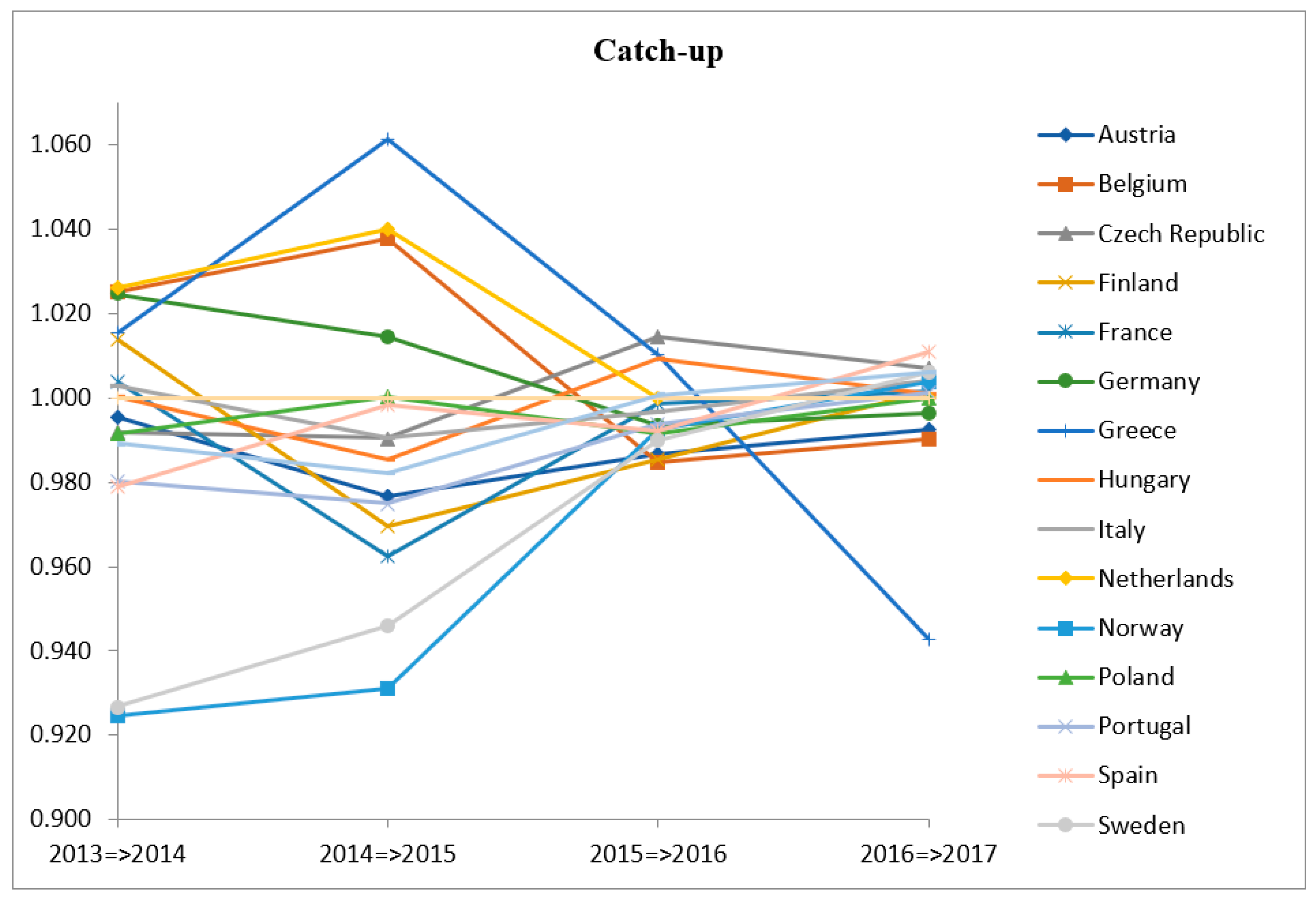
SD	0.029	0.033	0.009	0.015	0.014

shows the year-on-year efficiency changes (or catch-up effect) for the 17 DMUs from 2013 to 2017. Figure 2 shows a diagram of the results.

From 2013 to 2014, seven countries were found to have improved efficiency—the Netherlands, Belgium, Finland, France, Germany, Greece, and Italy (with a greater-than-1 efficiency change score). This implies that these seven countries improved the use of inputs to produce more desired output (GDP) and lesser undesired output (CO₂). Among the seven countries, the Netherlands had the best improvement (+2.6%). However, the improvements made by these seven countries are minor. There are two countries (Hungary and Switzerland) with no change. The remaining eight countries recessed in their efficiency. They are Austria, the Czech Republic, Norway, Poland, Portugal, Spain, Sweden, and the United Kingdom, due to a less-than-1 efficiency change score. Among the eight countries, Norway recessed the most (−7.5%), followed by Sweden (−7.3%). From 2013 to 2014, the 17 countries as a whole improved 0.6%.

From 2014 to 2015, 4 countries are found to have improved efficiency. They are Greece, Belgium, Germany, and the Netherlands (with a greater-than-1 efficiency change score). Among these four countries, Greece improved the most (+6.9%). Another three countries recessed. They were Finland, France, and Italy. Two countries (Poland and Switzerland) kept no change in their efficiency. There are 11 countries with deteriorated efficiency—Austria, the Czech Republic, Finland, France, Hungary, Italy, Norway, Portugal, Spain, Sweden, and the United Kingdom (with a less-than-1 efficiency change score). However, the number of recessing countries increases to 11 from 7. Among the 11 countries, Norway once again recessed the most (−6.9%). From 2014 to 2015, the 17 countries as a whole recessed 0.8%.

From 2015 to 2016, four countries were found to have improved efficiency. They are the Czech Republic, Hungary, Greece, and the United Kingdom (with a greater-than-1 efficiency change score). Among them, the Czech Republic is the countries with the best improvement (+1.5%). Two other countries, the Netherlands and Hungary, had no change on their efficiency. The rest 11 countries had a regressive efficiency. They are Austria, Belgium, Finland, France, Germany, Italy, the Netherlands, Norway, Poland, Portugal, Spain, Sweden, and Switzerland (with a less-than-1 efficiency change score). Among the 11 countries, Belgium had the worst regression (−1.5%). However, the regressions and improvements of these countries are minor. From 2015 to 2016, the 17 countries as a whole recessed 0.3%.

From 2016 to 2017, 10 countries are found to have improved (from 4 to 10). They are Spain, Czech Republic, Finland, France, Hungary, Italy, Norway, Portugal, Sweden and United Kingdom. This implies more countries can better use inputs to produce more desired output (GDP) and less undesired output (CO₂ emissions). Among the 10 countries, Spain improved the most (+1.1%). Three countries (the Netherlands, Poland and Switzerland) kept no change on their efficiency. 4 countries had recessed efficiency. They are Austria, Belgium, Germany and Greece. Among the 4 countries, Greece recessed the most (−5.7%). From 2016 to 2017, the 17 countries as a whole recessed 0.2%.

The last column in Table 6 shows the overall average efficiency changes of DMUs during 2013–2017. These values range between 0.963 and 1.017. The overall average efficiency change of all 17 countries in this time period is 0.995, which shows a minor recession. The efficiency in the time period recessed the most (−0.8%) in the time period 2014–2015 and improved the most (−0.2%) in the time period 2016–2017.

It is also noted that in 2013–2017 Austria continuously deteriorated technological efficiency while Switzerland stayed unchanged and Netherlands had the best improvement (+1.7%). Greece suffered a higher regression in efficiency change from 2014–2017. Except for the Greece, other counties, after 2015, had a quite stable efficiency.

5.2.2. Technological Change

Table 8. Year-on-year technological efficiency change for the 17 DMUs from 2013 to 2017.

DMU	2013–2014	2014–2015	2015–2016	2016–2017	Average
Austria	1.041	0.984	1.000	0.993	1.004
Belgium	0.946	0.951	0.997	0.995	0.972
Czech Republic	0.984	0.980	0.984	1.004	0.988
Finland	1.020	0.995	1.002	0.983	1.000
France	1.056	0.960	1.000	0.994	1.002
Germany	0.968	0.972	0.998	0.990	0.982
Greece	0.996	0.996	0.994	0.981	0.992
Hungary	1.008	0.992	0.992	0.989	0.995
Italy	1.053	0.956	0.976	0.993	0.994
Netherlands	0.920	0.936	0.988	1.001	0.961
Norway	1.059	0.973	0.999	0.997	1.007
Poland	0.997	0.981	0.986	1.000	0.991
Portugal	1.005	0.996	0.978	0.978	0.989
Spain	1.017	0.993	0.999	0.978	0.997
Sweden	1.062	0.981	1.004	0.990	1.010
Switzerland	1.038	1.000	1.004	0.998	1.010
United Kingdom	0.993	0.970	0.999	0.993	0.989
Average	1.010	0.977	0.994	0.992	0.993
Max	1.062	1.000	1.004	1.004	1.010
Min	0.920	0.936	0.976	0.978	0.961
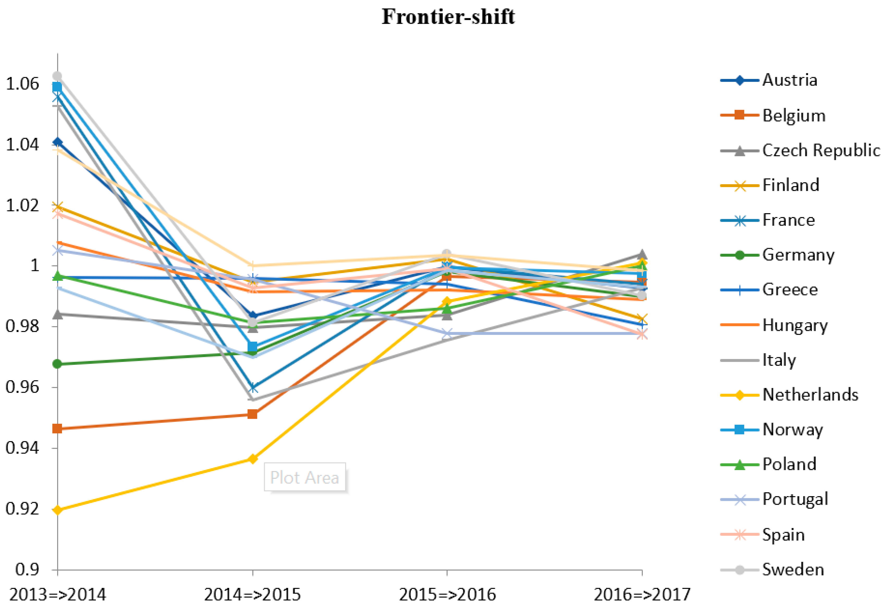
SD	0.041	0.018	0.009	0.008	0.013

shows the year-on-year technological changes or “frontier-shift effect” for 17 DMUs from 2013 to 2017. Figure 3 shows the diagram.

From 2013 to 2014, 10 countries are found to have improved technological efficiency. They are Austria, Finland, France, Hungary, Italy, Norway, Portugal, Spain, Sweden, and Switzerland. This implies these countries have innovated and improved their technologies for production. Among these countries, Sweden improved its technology the most (+6.2%). However, seven countries were found to have a recessed technology efficiency, including Belgium, the Czech Republic, Germany, Greece, the Netherlands, Poland, and the United Kingdom, each of them with a less-than-1 technological change score. The Netherlands recessed technological efficiency the most (−8%). From 2013 to 2014, the 17 countries as a whole improved 1%.

From 2014 to 2015, the number of countries with improved technological efficiency was down to 0 from 10, a big drop. Switzerland had no change on the technological efficiency (due to a technological efficiency change score = 1). The other rest 16 countries recessed in their technological efficiency. They are Austria, Belgium, Czech Republic, Finland, France, Germany, Greece, Hungary, Italy, the Netherlands, Norway, Poland, Portugal, Spain, Sweden, the United Kingdom (with a less-than-1 technological efficiency change score). Among them, the Netherlands recessed the most (−6.3 %). In this time period, the 17 countries as a whole recessed 0.23%.

From 2015 to 2016, the number of countries with improved technological efficiency increases from 0 to 3. They are Finland, Sweden, and Switzerland (with a greater-than-1 technological change score). Switzerland continued to advance its technological efficiency; together with Sweden, Switzerland had the best technological efficiency improvement (+4%). However, the improvements made by these countries are not significant. Two countries had no change to technological efficiency in this time period. They are Austria and France. The remaining 12 countries had regressive technological efficiency. They are Belgium, the Czech Republic, Germany, Greece, Hungary, Italy, the Netherlands, Norway, Poland, Portugal, Spain, and the United Kingdom (with a less-than-1 technological efficiency change score). Among the 12 countries, Italy was the country with the worst regression (−2.4%). However, these improvements and regressions were found to be minor, as the best improvement is 0.4%, while the worst regression is 2.4%. As a whole, 17 countries recessed 0.6% in this time period.

From 2016 to 2017, three countries had improved technological efficiency—the Czech Republic, the Netherlands, and Poland (with a greater-than-1 technological efficiency change score). Switzerland failed to advance its technological efficiency in this time period. However, the improvements made by these three countries were found to be minor. Poland was the only country with no change to efficiency in this time period. The number of countries with regressive technological efficiency increase from 12 to 13. The 13 countries were Austria, Belgium, Finland, France, Germany, Greece, Hungary, Italy, Norway, Portugal, Spain, Sweden, the United Kingdom, and Switzerland (with a less-than-1 technological efficiency change score). Among the 13 countries, Portugal and Spain were the countries with the worst technological efficiency recession (−2.2%). However, these improvements and regressions were found to be minor, as the best improvement is 0.39%, while the worst regression was 2.9%. As a whole, the 17 countries recessed 0.8% in this time period.

The last column in Table 7 lists the average technological changes of DMUs in the whole period (2013–2017). The values of range between 0.970 and 1.010. However, the overall average efficiency change score of all countries in the whole time period was 0.993, which was a minor recession (−0.7%). The technology efficiency of these countries improved the most (+1%) in the time period 2013–2014 and recessed the most (−2.3%) in the time period 2014–2015. This implies there was a lack of improving technologies for production from 2014–2015. After 2014, the technological efficiency of the 17 countries recessed stably and slightly.

5.2.3. MPI Change

Table 9. Year-on-year MPI changes for the 17 DMUs from 2013 to 2017.

DMU	2013–2014	2014–2015	2015–2016	2016–2017	Average
Austria	1.036	0.961	0.987	0.985	0.992
Belgium	0.970	0.987	0.981	0.985	0.981
Czech Republic	0.976	0.970	0.998	1.011	0.989
Finland	1.034	0.965	0.988	0.984	0.993
France	1.060	0.924	0.998	0.996	0.994
Germany	0.992	0.986	0.992	0.987	0.989
Greece	1.012	1.057	1.004	0.925	0.999
Hungary	1.008	0.977	1.001	0.990	0.994
Italy	1.056	0.947	0.972	0.997	0.993
Netherlands	0.944	0.974	0.988	1.001	0.977
Norway	0.979	0.906	0.992	1.001	0.970
Poland	0.989	0.982	0.978	1.000	0.987
Portugal	0.985	0.971	0.972	0.979	0.977
Spain	0.996	0.991	0.992	0.988	0.992
Sweden	0.985	0.928	0.994	0.996	0.976
Switzerland	1.038	1.000	1.004	0.998	1.010
United Kingdom	0.982	0.953	0.999	0.999	0.983
Average	1.002	0.969	0.991	0.990	0.988
Max	1.060	1.057	1.004	1.011	1.010
Min	0.944	0.906	0.972	0.925	0.970
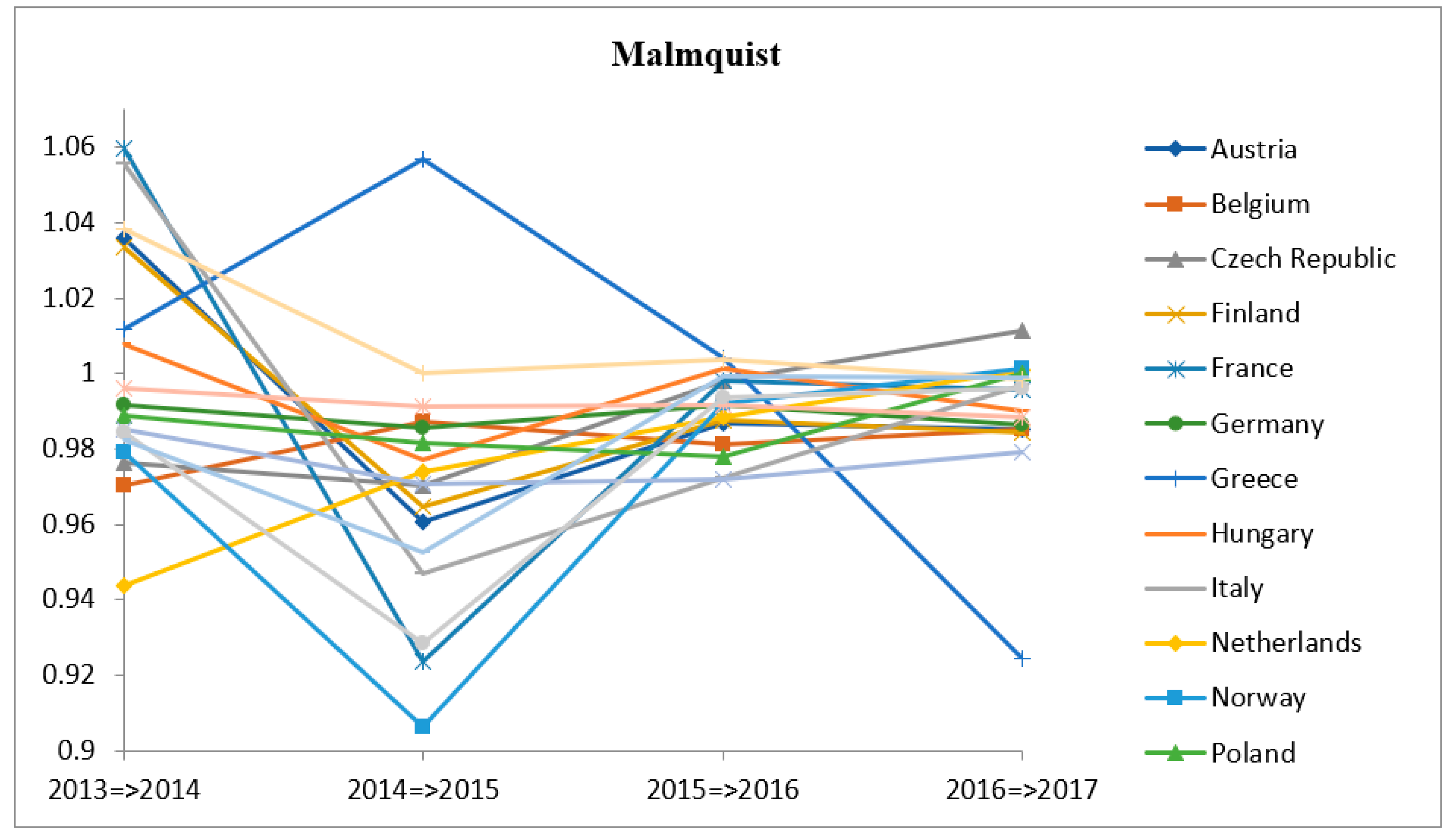
SD	0.032	0.034	0.010	0.019	0.010

shows the year-on-year MPI changes for the 17 DMUs from 2013 to 2017. Figure 4 shows the diagram.

From 2013 to 2014, 7 countries are found to have improved productivity. They are Austria, Finland, France, Greece, Hungary, Italy and Switzerland (with a greater-than-1 MPI change score). Among the 7 countries, France improved productivity the most (6.05%). 10 countries are found to have recessed productivity. They are Austria, Belgium, the Czech Republic, Germany, Hungary, Italy, the Netherlands, Norway, Poland, Portugal, Spain, Sweden, United Kingdom, and Switzerland (with MPI change score < 1). Among them, the Netherlands recessed the most (−5.6%). In this time period, the 17 countries as a whole recessed 0.2%.

From 2014 to 2015, 1 country is found to have improved productivity, down from 7, a big dip. It is Greece with an improvement of 5.7%. The country, Switzerland, kept no change. Another 15 countries, Austria, Belgium, Czech Republic, Finland, France, Germany, Hungary, Italy, the Netherlands, Norway, Poland, Portugal, Spain, Sweden, and United Kingdom recessed. Among them, Norway recessed the most (−9.4%). In this time period, the 17 countries as a whole recessed 3.1%.

From 2015 to 2016, 3 countries are found to have improved productivity, increased from 1. They are Greece, Hungary and Switzerland. Among the 3 countries, Greece improved productivity the most (+0.4%). The remaining 14 countries are with recessed productivity. They are Austria, Belgium, the Czech Republic, Finland, France, Germany, Italy, the Netherlands, Norway, Poland, Portugal, Spain, Sweden, and the United Kingdom. Among the 14 countries, Italy rexes the most (+2.8%). In this time period, the 17 countries as a whole recessed 0.9%.

From 2016 to 2017, 3 countries are found to have improved productivity. They are Czech Republic, Netherlands and Norway. Among them, Czech Republic improved the most (+11%). Poland kept no change. The remaining 13 countries had recessed productivity. They are Austria, Belgium, Finland, France, Germany, Greece, Hungary, Italy, Poland, Portugal, Spain, Sweden, United Kingdom, and Switzerland. Among them, Greece recessed the most (−7.5%). In this time period, the 17 countries as a whole recessed 0.1%.

In summary, the overall average MPI change score (0.988) shows a minor of 1.2% regression in total productivity for these 17 countries as a whole. The year-on-year productivity changes from 2013 to 2017 are found quite stable. From 2014 to 2015 the overall average productivity dipped and the number of improved countries decreases to 1 from 7. Nevertheless, the number of improved countries recovered back to 3 in the next time period from 2015 to 2016. Among these improved countries, Greece improved the most. After this time period, Greece had a big recession while others improved.

Table 10. Average MPI changes and its components from 2013–2017.

Dmu	Average Efficiency Change	Average Technological Change	Average Mip Change
Austria	0.952	1.014	0.965
Belgium	1.037	0.878	0.910
Czech Republic	1.004	0.954	0.958
Finland	0.970	0.996	0.967
France	0.966	1.005	0.971
Germany	1.029	0.930	0.957
Greece	1.027	0.984	1.010
Hungary	0.996	0.984	0.980
Italy	0.994	0.989	0.983
Netherlands	1.067	0.836	0.892
Norway	0.858	1.024	0.879
Poland	0.984	0.964	0.948
Portugal	0.951	0.954	0.907
Spain	0.980	0.971	0.952
Sweden	0.873	1.030	0.899
Switzerland	1.000	0.998	0.998
United Kingdom	0.978	0.958	0.937
Average	0.980	0.969	0.948

presents the results of these MPIs for the 17 companies in the time period 2013–2017.

Table 9 shows that the average MPI changes for the 17 countries range from 1% to −12.1%. Among them, Greece improved its productivity the most (+1%), while Norway had the worst productivity recession (−12.1%). From 2013 to 2017, Greece was the only country with an improved productivity change. In the whole time period, the overall average MPI change for all countries was −5.2%.

6. Conclusions and Future Research Direction

In this study, SBM DEA was used to assess the eco-efficiency for 17 European countries in the time period 2013–2017. For this assessment, energy consumption per capita and share of renewable energy in total energy consumption were selected as energy inputs, while labor productivity and gross capital formation were selected as economic inputs. On the other hand, GDP per capita was selected as a desired output, while CO₂ emissions per capita was selected as an undesired output.

The experimental results reveal the relative eco-efficiency of the 17 countries. In this time period, nine of the 17 countries were found to have the best eco-efficiency score of 1, including France, Hungary, Greece, Italy, the Netherlands, Poland, Portugal, Switzerland, and the United Kingdom. The other eight countries—Austria, Belgium, the Czech Republic, Finland, Germany, Norway, Spain, and Sweden—had relatively lower eco-efficiencies, with their scores ranging between 0.559 and 0.704. The 17 countries have an overall average efficiency change score of 0.995, which indicates a 0.5% minor recession. The overall average technological efficiency score (0.993) shows the 17 countries as a whole had a 0.7% regression. The overall average MPI change score (0.988) shows that the 17 countries as a whole had a 1.2% regression.

Some management implications are derived. First, the eco-efficiency scores reveal the efficiency of each country and those countries with poor efficiency certainly need to improve their efficiency. However, the countries with the best efficiency still need to improve their eco-efficiency, as the eco-efficiency scores derived in this research are relative values. Second, the results show that these countries had a minor recession in efficiency change, so these countries need to improve their efficiency. Third, as the results show that these countries had a minor recession in technological efficiency, these countries therefore need to better innovate and develop technologies to improve their production. Finally, the MPI scores show that the loss of productivity mainly comes from the lack of technological efficiency, so improving technological efficiency is therefore the first priority for these countries.

The following policy implications are derived: (1) As the increase of renewable energy can reduce CO₂ emissions, European governments should encourage the use of renewable energy. (2) Subsidy policy on the use of renewable energy can be used as an incentive. (3) As the use of fossil fuels leads to the increase of CO₂ emissions, a higher tax should be imposed on their use in order to prevent the continued use of this kind of energy. (4) The National Renewable Energy Action Plans should be promoted to all European countries in order to accomplish the aims of the European Environment Policies.

The following research directions can be focused on in the future. First, due to the unavailability of data, this research only includes 17 countries, and therefore it cannot give a whole view on the whole European countries. Therefore, including more European countries can be one research direction. Second, in this study, we only considered one undesired output (CO₂). More undesired outputs, such as PM2.5 (ton) and waste (ton), can be considered and included in future research. Third, comparing the results to those obtained from other approaches can be performed in future research. Finally, we found that the input and output variables used in this research may suffer from the problem of multicollinearity, as there is some high correlation between X1 and X 2 (0.76), X1 and X3 (0.63), and X1 and X4 (0.67), which suggests that two types of inputs might be enough. The study of the impact of multicollinearity on these results should be investigated further.

References

1. Huppes, G.; Mansanobu, I. Quantified Eco-Efficiency: An Introduction with Applications; Springer: London, UK, 2007; Volume 22. [Google Scholar]
2. Yadong, Y. Eco-efficiency trends in china, 1978–2010: Decoupling environmental pressure from economic growth. Ecol. Indic. 2013, 24, 177–184. [Google Scholar] [CrossRef]
3. OECD. Indicators to Measure Decoupling of Environmental Pressure from Economic Growth. Sustainable Development. Available online: http://www.docstoc.com/docs/84838188/oecd_decoupling (accessed on 13 March 2019).
4. European Commission. Communication from the Commission to the EU Parliament, the Council, the European Economic and Social Committee, the Committee of the Regions and the European Investment Bank, Closing the Loop—An EU Action Plan for the Circular Economy. Available online: http://eurlex.europa.eu/resource.html?uri=cellar:8a8ef5e8-99a0-11e5-b3b7-01aa75ed71a1.0012.02/DOC_2&format=PDF (accessed on 13 March 2019).
5. European Commission. Energy Union Package—A Framework Strategy for a Resilient Energy Union with a Forward-Looking Climate Change Policy. Available online: http://eur-lex.europa.eu/resource.html?uri=cellar:1bd46c90-bdd4-11e4-bbe1-01aa75ed71a1.0001.03/DOC_1&format=PDF (accessed on 13 March 2019).
6. European Commission. Communication from the Commission, EU2020—A Strategy for Smart, Sustainable and Inclusive Growth. Available online: http://eurlex.europa.eu/LexUriServ/LexUriServ.do?uri=COM:2010:2020:FIN:EN:PDF (accessed on 13 March 2019).
7. European Commission. EU Resource Efficiency Scoreboard. 2015. Available online: http://ec.europa.eu/environment/resource_efficiency/targets_indicators/scoreboard/pdf/EU%20Resource%20Efficiency%20Scoreboard%202015 (accessed on 13 March 2019).
8. European Commission. Roadmap to a Resource Efficient Europe. Available online: http://eurlex.europa.eu/legalcontent/EN/TXT/PDF/?uri=CELEX:52011DC0571&from=EN (accessed on 13 March 2019).
9. Muradin, M.; Katarzyna, J.L.; Foltynowicz, Z. Evaluation of Eco-Efficiency of Two Alternative Agricultural Biogas Plants by Magdalena Muradin. Appl. Sci. 2018, 8, 2083. [Google Scholar] [CrossRef] [Green Version]
10. Hadad, Y.; Keren, B.; Hanani, M.Z. Combining data envelopment analysis and Malmquist Index for evaluating police station efficiency and effectiveness. Police Pract. Res. 2015, 16, 5–21. [Google Scholar] [CrossRef]
11. Farrell, M.J. The Measurement of Productive Efficiency. J. R. Stat. Soc. 1957, 120, 253–290. [Google Scholar] [CrossRef]
12. Charnes, A.; Cooper, W.W.; Rhodes, E. Measuring the efficiency of decision-making units. Eur. J. Oper. Res. 1978, 2, 429–444. [Google Scholar] [CrossRef]
13. Banker, R.D.; Charnes, A.; Cooper, W.W. Some Models for Estimating Technical and Scale Inefficiencies in Data Envelopment Analysis. Manag. Sci. 1984, 30, 1078–1092. [Google Scholar] [CrossRef] [Green Version]
14. Liu, Z.; Zhuang, J. Evaluating Partial Reforms in the Chinese State Industrial Sector: A stochastic frontier cost function approach. Int. Rev. Appl. Econ. 1998, 12, 9–24. [Google Scholar] [CrossRef]
15. Charnes, A.; Cooper, W.W.; Lewin, A.; Seiford, L. Data Envelopment Analysis Theory. Methodol. Appl. 1997, 48, 1997. [Google Scholar]
16. Dyson, R.G.; Allen, R.; Camanho, A.S.; Podinovski, V.V.; Sarrico, C.S.; Shale, E.A. Pitfalls and protocols in DEA. Eur. J. Oper. Res. 2001, 132, 245–259. [Google Scholar] [CrossRef]
17. Ramli, N.A.; Munisamy, S. Modeling Undesirable Factors in Efficiency Measurement Using Data Envelopment Analysis: A Review. J. Sustain. Sci. Manag. 2013, 8, 126–135. [Google Scholar]
18. Scheel, H. Undesirable outputs in efficiency valuations. Eur. J. Oper. Res. 2001, 132, 400–410. [Google Scholar] [CrossRef]
19. Koopmans, T.C. Analysis of Production as an Efficient Combination of Activities. Act. Anal. Prod. Alloc. 1951, 36, 27–56. [Google Scholar]
20. Tyteca, D. Linear Programming Models for the Measurement of Environmental Performance of Firms-Concepts and Empirical Results. J. Prod. Anal. 1997, 8, 183–197. [Google Scholar] [CrossRef]
21. Seiford, L.M.; Zhu, J. Modeling Undesirable Factors in Efficiency Evaluation. Eur. J. Oper. Res. 2002, 142, 16–20. [Google Scholar] [CrossRef]
22. Iqbal, A.; Seiford, L.M. Translation Invariance in Data Envelopment Analysis. Oper. Res. Lett. 1990, 9, 403–405. [Google Scholar] [CrossRef]
23. Färe, R.; Grosskopf, S.; Lovell, C.A.K.; Pasurka, C. Multilateral Productivity Comparisons When Some Outputs are Undesirable: A Non-Parametric Approach. Rev. Econ. Stat. 1989, 71, 90–98. [Google Scholar] [CrossRef]
24. Zhou, P.; Ang, B.W.; Poh, K.L. Slacks-based Efficiency Measures for Modeling Environmental Performance. Ecol. Econ. 2006, 60, 111–118. [Google Scholar] [CrossRef]
25. Tone, K. A slacks-based measure of efficiency in data envelopment analysis. Eur. J. Oper. Res. 2001, 130, 498–509. [Google Scholar] [CrossRef] [Green Version]
26. Chung, Y.H.; Färe, R.; Grosskopf, S. Productivity and Undesirable Outputs: A DDF Approach. J. Environ. Manag. 1997, 51, 229–240. [Google Scholar] [CrossRef] [Green Version]
27. Portela, M.C.A.S.; Thanassoulis, E.; Simpson, G. Negative Data in DEA: A Directional Distance Approach Applied to Bank Branches. J. Oper. Res. Soc. 2004, 55, 1111–1121. [Google Scholar] [CrossRef] [Green Version]
28. Fukuyama, H.; Weber, W.L. A Slacks-based Inefficiency Measure for A Two-stage System with Bad Outputs. Omega 2010, 38, 398–409. [Google Scholar] [CrossRef]
29. Färe, R.; Grosskopf, S. Directional Distance Functions and Slacks-based Measures of Efficiency. Eur. J. Oper. Res. 2010, 200, 320–322. [Google Scholar] [CrossRef]
30. Choi, Y.; Zhang, N.; Zhou, P. Efficiency and abatement costs of energy-related CO2 emissions in China: A slacks-based efficiency measure. Appl. Energy 2012, 98, 198–208. [Google Scholar] [CrossRef]
31. Lee, T.W.; Yeo, G.T.; Thai, V. Environmental efficiency analysis of port cities: Slacks-based measure data envelopment analysis approach. Transp. Policy 2014, 33, 82–88. [Google Scholar] [CrossRef]
32. Camioto, F.C.; Moralles, H.F.; Mariano, E.B.; Rebelatto, D. Energy efficiency analysis of G7 and BRICS considering total-factor structure. J. Clean. Prod. 2016, 122, 67–77. [Google Scholar] [CrossRef]
33. Hadad, Y.; Hanani, M.Z. Combining the AHP and DEA methodologies for selecting the best alternative. Int. J. Logist. Syst. Manag. 2011, 9, 251. [Google Scholar] [CrossRef]
34. Bian, Y.W.; Yang, F. Resource and environment efficiency analysis of provinces in China: A DEA approach based on Shannon’s entropy. Energy Policy 2010, 38, 1909–1917. [Google Scholar] [CrossRef]
35. Robaina-Alves, M.; Moutinho, V.; Macedo, P. A new frontier approach to model the eco-efficiency in European countries. J. Clean. Prod. 2015, 103, 562–573. [Google Scholar] [CrossRef] [Green Version]
36. Moutinho, V.; Madaleno, M.; Robaina, M. The economic and environmental efficiency assessment in EU cross-country: Evidence from DEA and quantile regression approach. Ecol. Indic. 2017, 78, 85–97. [Google Scholar] [CrossRef]
37. Moutinho, V.; Jose, F.; Antonio, M.; Renato, S. Assessing eco-efficiency through the DEA analysis and decoupling index in the Latin America countries. J. Clean. Prod. 2018, 205, 512–524. [Google Scholar] [CrossRef]
38. Halkos, G.; Petrou, K.N. Assessing 28 EU member states’ environmental efficiency in national waste generation with DEA. J. Clean. Prod. 2019, 208, 509–521. [Google Scholar] [CrossRef]
39. Wang, T.L.; Yang, J.Y.; Wang, K.D. Measurement and evolution of eco-efficiency of coal industry ecosystem in China. J. Clean. Prod. 2019, 209, 803–818. [Google Scholar] [CrossRef]
40. Tone, K.A. Dealing with Undesirable Outputs in DEA: A Slacks-Based Measure (SBM) Approach. 2013. Available online: https://www.researchgate.net/publication/284047010_Dealing_with_undesirable_outputs_in_DEA_a_Slacks-Based_Measure_SBM_approach (accessed on 13 March 2019).
41. Walter, D.; Douglas, W.C.; Laurits, R.C. The Economic Theory of Index Numbers and the Measurement of Input, Output, and Productivity. Econometrica 1982, 50, 1393–1414. [Google Scholar]
42. Malmquist, S. Index number and indifference surfaces. Trab. Estat. 1953, 4, 209–242. [Google Scholar]
43. Färe, R.; Grosskopf, S.; Norris, M.; Zhang, Z. Productivity Growth, Technical Progress and Efficiency Change in Industrialized Countries. Am. Econ. Rev. 1994, 1, 66–83. [Google Scholar]
44. World Bank. Available online: https://data.worldbank.org (accessed on 13 March 2019).
45. Enerdata Year Book. Available online: https://yearbook.enerdata.net (accessed on 13 March 2019).
Figure 1. A structure of Data Envelopment Analysis (DEA) efficiency measurement with undesired output.
Applsci 10 01760 g001
Figure 2. Year-on-year efficiency changes from 2013 to 2017.
Applsci 10 01760 g002
Figure 3. Yearly technological changes from 2013 to 2017.
Applsci 10 01760 g003
Figure 4. Year-on-year productivity changes (Malmquist Productivity Index–MPI) from 2013 to 2017.
Applsci 10 01760 g004