Abstract
Due to the rapid development of shale gas, a system has been established that can utilize a considerable amount of data using the database system. As a result, many studies using various machine learning techniques were carried out to predict the productivity of shale gas reservoirs. In this study, a comprehensive analysis is performed for a machine learning method based on data-driven approaches that evaluates productivity for shale gas wells by using various parameters such as hydraulic fracturing and well completion in Eagle Ford shale gas field. Two techniques are used to improve the performance of the productivity prediction machine learning model developed in this study. First, the optimal input variables were selected by using the variables importance method (VIM). Second, cluster analysis was used to analyze the similarities in the datasets and recreate the machine learning models for each cluster to compare the training and test results. To predict productivity, we used random forest (RF), gradient boosting tree (GBM), and support vector machine (SVM) supervised learning models. Compared to other supervised learning models, RF, which is applied with the VIM, has the best prediction performance. The retraining model through cluster analysis has excellent predictive performance. The developed model and prediction workflow are considered useful for reservoir engineers planning of field development plan.
1. Introduction
Since 2010, the multistage hydraulic fracturing for horizontal wells has been established as a method for producing shale gas and tight oil, especially in North America. As of 2018, shale gas accounted for over 50% of total natural gas production in the US (Figure 1) [1]. Future production profiles and estimated ultimate recovery (EUR) of shale gas wells are obtained by such methods as reservoir simulation [2], hydraulic fracturing modeling, rate transient analysis (RTA), and decline curve analysis (DCA). However, the reservoir simulation implies high uncertainty in representing flow behavior due to reservoir properties, complexity of reservoir, absorption or desorption flow, and variation of fracture permeability [3,4,5,6,7]. It is a time-consuming and a challenge task. In case of RTA, data of flow pressure and reservoir property over time are necessary, and the end of transient linear flow can be accurately predicted only by deriving the stimulated reservoir volume (SRV) through microseismic (MS) analysis. In this way, the estimated ultimate recovery (EUR) can be calculated [8]. However, property data are difficult to acquires, and the MS analysis implies uncertainty, which are the disadvantages of RTA. For this reason, many studies have actively attempted to apply a DCA in order to predict the productivity of a shale reservoirs.
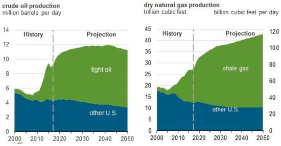
Figure 1.
Shale gas production includes associated natural gas from tight oil plays.
The DCA method proposed by Arps [9] has been widely applied to traditional oil and gas reservoirs. This method assumes the pseudo steady state flow. However, shale gas has low permeability and is produced in hydraulic fractured horizontal wells, which delays the entry into the boundary dominated flow (BDF) regime. Accordingly, it is not possible to forecast a production profile by using initial production data. Some studies proposed new decline curve analysis methods considering production profiles of shale and tight reservoirs (super-hyperbolic decline method; superbolic, power law exponential decline method; PLE, modified-stretched exponential decline; YM-SEPD, Duong method, logistic growth model; LGM) [10,11,12,13,14]. However, these DCA methods tend to over and underestimate production rates due to the difference among various flow characteristics like reservoir property, hydraulic fracturing design, and natural fracture network. To overcome the above weakness, a study [15] was also conducted to propose a cumulative production incline rate index that selects an appropriate DCA methods.
However, the DCA methods requires at least one year of production data. Shale reservoirs have a reported economic recovery of three years and require a model that can know the productivity of the wells to be developed before drilling or early stage of production.
To overcome the limitations of simulation and DCA methods, machine learning techniques were studied and applied by many researchers for predicting productivity in shale and tight reservoirs. Mohaghegh [16] quantitatively assessed the impact of shale gas development by conducting pattern recognition analysis and analyzing the correlation between productivity and other factors like rock mechanical property, hydraulic fracturing and well completion data, and reservoir property. Zhong et al. [17] predicted the cumulative production rate of the Wolfcamp reservoir in USA by using various supervised learning techniques, such as regression analysis, support vector machine (SVM), and gradient boosting machine (GBM). In addition, the classification and regression tree (CART) using regression analysis was performed to identify the importance of input data and select useful input data for productivity. This attempt aimed to improve the prediction performance of a model.
Clustering analysis is one of unsupervised learning techniques. This technique measures the similarity of datasets and classifies target groups in order to identify similarity of objects belonging to the same group and difference among groups. In oil engineering, the clustering analysis is mainly used to estimate electrofacies, classify properties in nonlinear relationships, and improve the accuracy of a prediction model. Sfidari et al. [18] applied an artificial intelligence-based clustering analysis (self-organizing map: SOM) and hierarchical k-means clustering analysis to classify electrofacies and thus predict total organic contents (TOC) from logging data. This method turned out to be better than the conventional analysis. Jung et al. [19] developed a method of enhancing the reliability of history matching and a prediction model of production profiles by combining the clustering analysis and SVM.
Other studies utilized data-driven based supervised or unsupervised learning to predict productivity in unconventional reservoirs, where fluid has a more complex flow pattern and different production methods are applied in comparison with conventional reservoirs. Bansal et al. [20] and Lolon et al. [21] obtained influential factors on shale gas productivity by using a statistical analysis model and proposed a data-based artificial neural network (ANN) model for predicting cumulative production rates. Alabbodi et al. [22], Mohaghegh et al. [23], and Li et al. [24] developed data-based ANN models to forecast the estimated ultimate recovery (EUR) of the Marcellus shale reservoir. They utilized not only Arps DCA method but also PLE, Duong, and SEPD methods to predict the EUR at the point of the minimum economic limit rate, which was selected as the input dataset. They also derived factors of the decline curve analysis methods by conducting the principal component analysis (PCA).
However, the above studies focused on eliciting parameters that affect productivity of shale reservoirs as input data for a supervised learning models and In addition, there are limitations in predicting the production profile and EUR using the parameters of DCA equations as output data.
In this paper, we have developed the supervised learning model that predicts the cumulative production using a data-driven approach and machine learning modeling for Eagle Ford shale reservoirs. The developed model can predict the cumulative production at various production times and can be useful for forecasting the productivity at a well in the early stage of production.
The main novel contributions of our paper can be summarized as follows:
- First, our work considers the overfitting problem caused by unnecessary input features of prediction models. To further enhance the predictive performance of our machine learning model, we performed an RF-based variables importance method and statistical analysis to eliminate unnecessary input features.
- Second, after removing input features using VIM, general supervised learning models, including random forest, gradient boosting tree, and support vector machine were evaluated, and we selected the best model to predict productivity in Eagle Ford shale reservoirs.
- Third, to enhance the prediction model performance, clustering analysis was used, and the supervised learning model for each cluster was re-trained and compared with the results.
2. Materials and Methods
Clustering refers to a very broad set of techniques for finding subgroups or clusters in a data set. When we cluster the observations of a data set, we seek to partition them into distinct groups so that the observations within each group are quite similar to each other, while observations in different groups are quite different from each other. Of course, to make this concrete, we must define what it means for two or more observations to be similar or different. Clustering is widely used in many fields and has many methods. The most common techniques are K-means clustering, Partitioning Around Medoids clustering and hierarchical clustering.
2.1. Random Forest
Random Forest is a machine learning technique that produces prediction values by constructing multiple decision trees [25]. Each decision tree constituting the random forest is constructed from training data and explanatory variables that are randomly extracted from the entire training data set. Because each decision tree has a different set of learned data, both the model of the tree constructed and the values predicted from it are different. Just as the learning data of one decision tree is formed differently in random forest, the unlearned data is extracted differently each time. Data not used in constructing decision trees is used for model validation (Figure 2). This is called OOB (Out-Of-Bag). The total number of OOB selections in the entire decision tree of the random forest is different for each individual entity, and the values that are classified when selected are also predicted differently for each tree. This feature allows us to calculate the probability of prediction for an individual entity. The advantage of this model is that, first, although the accuracy of a single tree may drop because the trained data set is small and but, the final accuracy predicted by combining them is superior to the simple decision tree algorithm. Second, according to the law of algebra, the larger the size of the forest (the number of trees), the more generalized errors, commonly known by the misclassification rate, converges to a certain limit value. Third, when retrieving individual decision trees, we use randomly reconstructed data from the entire learning data, so it is not affected by noise or outliers.
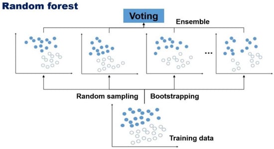
Figure 2.
Modeling process of random forest algorithm.
Where is the mean square error of the OOB data, is the number of trees in the forest, is the actual value, and is the predicted value for observation in the OOB data. and are the R-squared of the OOB data and the variance of the predicted parameters of the OOB data, respectively.
2.2. Gradient Boosting Tree
The proposal for the gradient rise comes from the concepts that it can be interpreted as an optimization algorithm for an appropriate cost function [26,27,28]. Afterwards, an explicit regression gradient rise algorithm was developed, which is a general functional gradient rise perspective, and then the research was upgraded in terms of algorithm enhancement as an iterative gradient drop algorithm. That is, the algorithm optimizes the cost function rather than the function space by repeatedly selecting the function (weak hypothesis) that points in the direction of the negative slope (Figure 3). These functional gradients have led to the development of algorithms beyond regression and classification in many areas of machine learning and statistics.
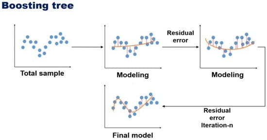
Figure 3.
Modeling process of boosting tree algorithm.
2.3. Support Vector Machine
Support vector machine (SVM) is a machine learning method proposed by Vapnik and Cortes [29]. It is one of the techniques widely used for classification and regression problems. SVM finds a set of hyperplanes in a space of high dimensional or infinite dimension and performs classification and regression analysis using it. SVM is a global classification model that utilizes all attributes and provides non-overlapping segmentation as a learning method. It is based on linear discrimination with SVM maximum margin and does not consider dependencies between attributes.
For the decision boundary function according to:
where w is the weight vector that defines the boundary and x, b represent the input vector, and the bias, respectively. The error function is as follows:
For training input vectors and target outputs, and are respectively the -th ( = 1, 2, 3, …, ) is referred to as input and output. And is a penalty with a constant greater than zero. This means that the penalty is given to , which is larger than the deviation of function . SVM efficiently performs nonlinear classification by using not only linear classification, but also mapping to a multidimensional space called a kernel trick. Intuitively, determining the decision boundary in the hyperplane shown in Figure 4 results in the lowest misclassification of new data when using the hyperplane with the largest margin as the classifier.
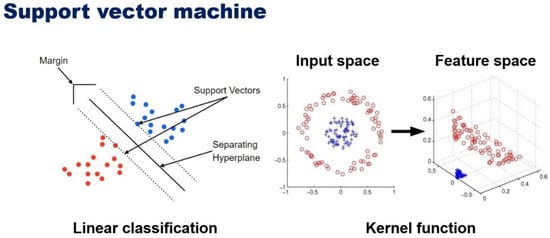
Figure 4.
Decision boundary function of SVM algorithm.
Thus, the model is changed into:
The kernel function is , which is represented by converting it back into a . are Lagrange multipliers, which allows the selection of various kernel functions suitable for regression analysis. For kernel functions, gaussian, hyperbolic tangent, and polynomial type can be used. Choosing the optimal kernel function parameters can prevent overfitting and improve predictive performance.
2.4. Clustering Analysis
2.4.1. K-means Clustering
K-means clustering is a simple and easy approach for partitioning a data set into K, non-overlapping clusters. It is the process of assigning observation values according to initial setting of values after setting the initial value. And minimizing the variance of the distance difference with each cluster. The main purpose of this analysis is to find a solution for satisfying the two objective functions that maximizes the degree of cohesion in the cluster and the separation between the clusters.
2.4.2. Partitioning Around Medoids Clustering
Partitioning Around Medoids (PAM or K-medoids) clustering is to select the real object data representing the cluster instead of averaging the distances of the observations. PAM clustering has two disadvantages, first, it is not valid for categorical data. Second, it is vulnerable to outliers. For PAM clustering, we use the median of the actual observations instead of using the center as an average in the cluster. Unlike the K-means clustering, it operates not only on the Euclidean distances but also on arbitrary distance functions.
2.4.3. Hierarchical Clustering
Hierarchical clustering is a method of forming clusters by repeating a process of grouping the most similar entities. Results are usually given in the form of dendrograms, with each individual belonging to only one cluster. Various definitions of similarity or distance between individuals are possible, and the results of clustering are derived differently according to the connection method between clusters. Generally, the Euclidean distance is used, where one has to make sure that all attributes have the same scale. This is a special case of the Minkowski distance with p. An agglomerative clustering algorithm starts with N groups, each initially containing one training instance and, merging similar groups to form larger groups, until there is a single one. A divisive clustering goes in the other direction, starting with a single group and dividing large groups into smaller groups, until each group contains a single instance. Hierarchical clusters have the advantage of being able to easily identify the structural relationships between clusters in the form of dendrograms. Through this, the distance between items and the distance between clusters can be known and the robustness of the cluster can be analyzed by checking the similarity between variables in the clusters.
2.5. Evaluating Prediction Models
In order to improve the accuracy of the developed ANN model, First, we used clustering in order to group the input data of the ANN model. Second, we carried out the variable importance analysis. Both methods selected the top 9 variables with high correlation among the input data. Statistical analysis was performed using the results of the pre-trained ANN model. The predicted results are compared based on the Mean Absolute Deviation (MAD), Mean Square Error (MSE), Root Mean Square Error (RMSE), Mean Absolute Percentage Error (MAPE), and coefficient of determination (R2), which is defined as Equations (7)–(11).
2.6. Evaluating Clustering Analysis
2.6.1. Connectivity
Let denote the total number of observations in the datasets and denote the total number of columns, which are assumed to be numeric. Define as the th nearest neighbor of observation , and let be zero if and are in the same cluster and otherwise. Then, for a particular clustering partition of the N observations into K disjoint clusters, the connectivity is defined as Equation (10). where is a parameter that represents the number of nearest neighbors. The connectivity has a value between zero and ∞ and should be minimized.
2.6.2. Dunn Index
Dunn index (DI) is another internal cluster evaluating metrics based on the clustered data itself. Equation (11) formulates DI, where denotes the distance between the two clusters while represents the distance between the nodes within the cluster. DI checks how dense the cluster is and how well it is separated from other clusters. For a given clustering formation, higher values of DI indicate better clustering.
2.6.3. Silhouette Coefficient
Silhouette coefficient (SC) checks for each node’s similarity with all the nodes in its own cluster and its dissimilarity from the nodes belonging to other clusters. In addition to giving a numeric value, SC can also provide a graphical representation of how well an object lies within its cluster. Equation (12) formulates silhouettes, where, is the average dissimilarity of node from the other nodes within the cluster. The value of is the minimum average dissimilarity of node to the nodes of all other clusters. The values from this function are in the range −1 to 1. A value of −1 indicates the worst possible clustering, while 1 specifies the best clustering. As follows:
In this work, data preprocessing and statistical analysis were conducted used the package library (‘ggplot’, ‘dplyr’) of R-program. And for learning and forecasting of supervised learning models, the statistics and machine learning toolbox in MATLAB (Math Works 2019a) was used.
3. Data Preparation and Description
3.1. Field Data for Developed Model
The study area includes dry gas and gas condensate at the Eagle Ford Shale Basin in Webb and La Salle counties, Texas, USA. The shale-play basins are distributed east to west in the area near the Gulf of Mexico, south of Texas (Figure 5). In the case of Eagle Ford Shale basin, the reserve of condensate tends to increase toward the north, while the southern area mainly produces dry gas. Vertically, the Eagle Ford Formation, which were deposited during the Cenomanian and Turonian ages of the Late Cretaceous, can be divided into the Lower and Upper Eagle Ford [30,31]. The Eagle Ford shale play is an important hydrocarbon source for Austin chalk on the Upper Eagle Ford. Locally, the Maness shale is identified at the bottom of the lower Eagle Ford shale with significantly higher gamma-ray and clay content than other parts of the Eagle Ford shale.
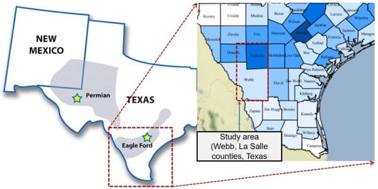
Figure 5.
The study area of Eagle Ford shale reservoirs.
3.2. Correlation Analysis
The Pearson correlation analysis between the variables used in this study showed that the highest value of 36 months of cumulative production used as a production variable was the result of the relative number of productivity variables, where the 3-month production rate is 0.761 MMscf and, peak for barrel of oil equivalent is 0.613 mbo, respectively. But, with the exception of the productivity variables, in summary, correlated hydraulic fracturing and well completion data including proppant volume (R = 0.527), slick water (R = 0.585), cluster (R = 0.347), lateral length (R = 0.341) can be used as input features to the productivity prediction model (Figure 6).
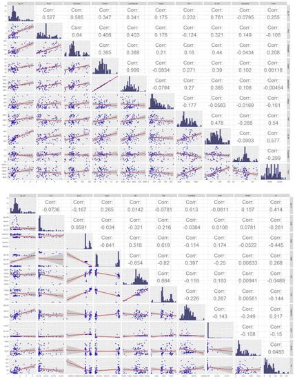
Figure 6.
Pearson correlation matrix and distribution of data used in the datasets.
3.3. Workflow for Developed Model
The developed model consisted of 129 horizontal wells (Webb—72 wells, LaSalle—57 wells) in the dry gas Eagle Ford Shale. The Drilling Info Webb site has been used to acquire the field data. Hydraulic fracturing, well completion, and reservoir property data related to productivity were determined as input data and the cumulative production of three years after production as an output data. The introduction and statistical analysis for inputs and targets parameters are presented in Table 1 and Table 2.

Table 1.
Parameters and abbreviation for input and target variables used in this study.
Table 2.
Statistical analysis of input and target variables datasets used in this study.
The workflow in Figure 7 show the three steps for productivity forecasting workflow. The first step is data preprocessing and preparation. To develop a supervised learning model, input variables and target variables need to be selected, and machine learning modeling need to be transformed into datasets that enable learning. In addition, outlier or null data that degrade the predictive performance of the model are removed. In the second step, application of machine learning modeling to improve predictive performance. First, The VIM based on RF prevents overfitting by eliminating low-correlation input features in the predictive model. Second, Clustering validity determines the number of clusters. It then re-generates the predictive model of clusters across the entire datasets for training. The third step is to use test data to compare the results between supervised learning models.
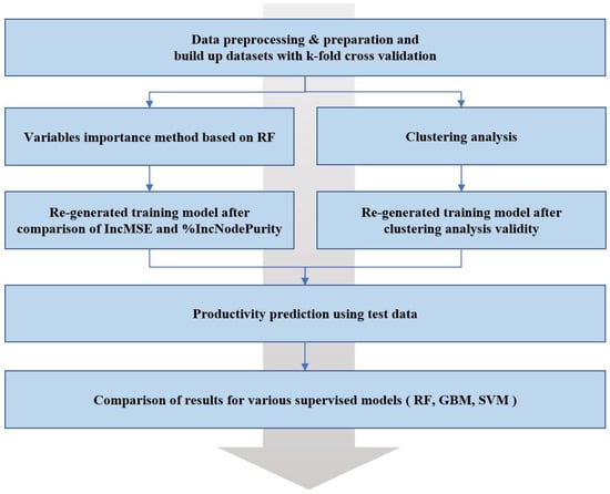
Figure 7.
Workflow of productivity forecasting development model for shale gas reservoirs.
4. Model Performance Analysis
4.1. Variables Importance Analysis
In constructing a regression analysis or machine learning supervised model, selecting variables that are highly correlated with target variables can prevent overfitting and reduce computation time.
The Pearson correlation is a method to analyze whether there is a linear relationship between response variables and input variables. In data mining, Pearson’s correlation is used to remove variables when the squared value is less than 0.005. However, there is a disadvantage in that only linear relationships can be identified. Recursive feature elimination with cross validation (RFE) is typically used for curvilinear or nonlinear relationships. In this work, we used RF-based regression analysis. In order to better predict 36-month cumulative production, rankings can be intuitively identified. The variables importance analysis method (VIM) is a critical output of the machine learning algorithm. For each variable in the matrix, it tells you how important that variable is in classifying the data. Generally, the plot shows each variable on the y-axis, and their importance on the x-axis. They are ordered top-to-bottom as most to least important. Therefore, the most important variables are at the top, and an estimate of their importance is given by the position of the dot on the x-axis. One should use the most important variables, as determined from the variable importance plot, in the principle component analysis (PCA), canonical discriminant analysis (CDA), or other analyses. Typically, you should look for a large break between variables to decide how many important variables to choose. This is an important tool for reducing the number of variables for other data analysis techniques, but you should be careful not to have either too few or too many variables.
In a regression tree analysis, RF uses %IncMSE and IncNodePurity to rank variable importance. %IncMSE is simply the average increase in squared residuals of the test set when variables are randomly permuted. When removing or adding a variable, if there is little change in the model, it is a importance. IncNodePurity is the increase in homogeneity in the data partitions.
The initial input features consisted of 18 independent variables. To perform input features ranking and finding variables importance, VIM based on random forest regression was used. Figure 8 demonstrates the results of input features ranking created by VIM (based on RF). The selected variables were mostly consistent with the findings in literature. According to the above results, both cases (VIM %IncMSE or IncNodePurity), for example, slick water, peak BOE, tubing head pressure, true vertical depth, lateral length, proppant volume, and initial production rate, correlate high enough for a 36-month cumulative production of shale reservoirs. As mentioned above, the results indicate that Qi_3M, Slickwater, and PeakBOE are three important variables, in which these variables account for over 50% of the importance of other variables and should be selected as the main variables when using this development model.
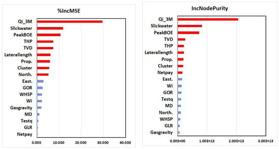
Figure 8.
Variable importance analysis results by random forest (%IncMSE and IncNodePurity).
4.2. Model Validation
Cross-validation (CV) is a resampling procedure used to evaluate machine learning models on a limited data sample. The procedure has a single parameter called k that refers to the number of groups that a given data sample is to be split into. As such, the procedure is often called k-fold CV. When a specific value for k is chosen, it may be used in place of k in the reference to the model, such as k = 5 becoming 5-fold CV (Figure 9). CV is one of the verification methods to further improve the predictive performance when new, largely untrained data is modeled as input to the training model. That is, to use a limited sample in order to estimate how the model is expected to perform in general when used to make predictions on data not used during the training of the model. This is generally more time consuming than other methods, such as simple train/test partitioning. However, it is a popular method because it prevents overfitting and does not result in biased or non-optimistic assumptions about model technology [32,33,34].
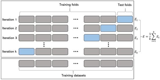
Figure 9.
Data partitioning scheme with K-fold validation.
4.3. Clustering Analysis for Datasets
It is important to estimate the number of K of clustering analysis in order to develop a robust re-generated supervised learning model [35]. We performed an analysis to find the optimal number of K from three clustering validity algorithms (Figure 10). First, using a connectivity index, it was found that the optimal number of k was two values for 3 cluster analysis. For K-means (C-index: 8.2) and PAM (C-index: 3.6) cluster algorithms, C-index looks similar on the graph, but more than twice as different from PAM, which shows better performance. Second, in the algorithm for calculating the number of K through the Dunn index value, the highest slope index was found in two. Finally, the optimal number of K was also calculated from the silhouette index value.
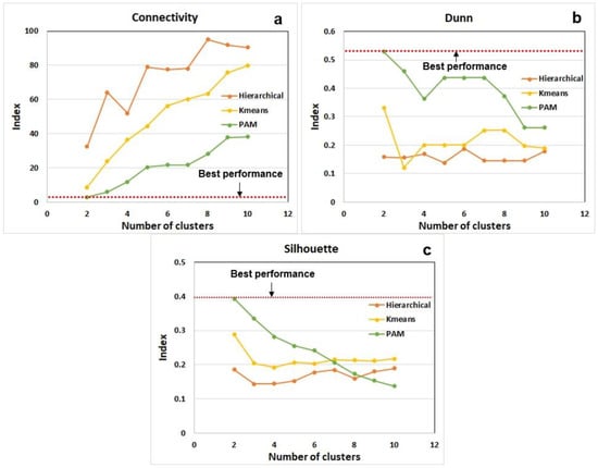
Figure 10.
Comparative performance of clustering validity analysis. (a) Connectivity (b) Dunn (c) Silhouette index.
Accordingly, best performance clustering is characterized by a lower C-index or a higher Dunn and Silhouette index values. It is understood that the PAM clustering provides the most efficient clustering compared to Hierarchical and K-means clustering analysis. Figure 11 shows the 9 input variables with two principal components (PC), the x-axis being PC 1 and the y-axis is PC 2. It represents the quantitative position coordinates of the yield values of whole production wells calculated by K-means clustering. The cluster 1 model of the blue circular point is distributed in the northwest direction from the center point, and the cluster 2 model is distributed in the southeast direction from the center point.
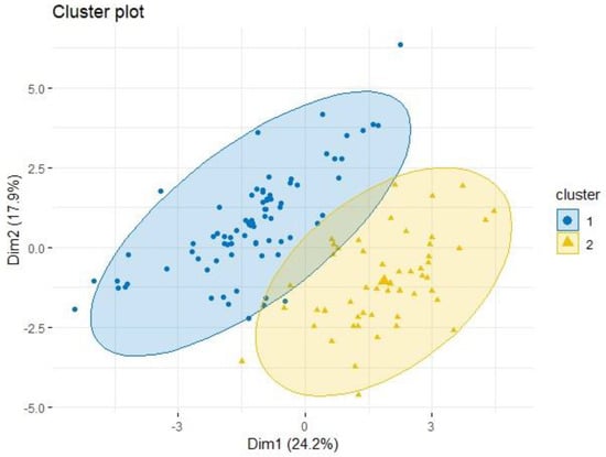
Figure 11.
Results of PAM clustering in principal component 1 and 2 cross plot.
5. Results and Discussions
It is very important for the machine learning algorithm to select the optimal hyperparameters. This can prevent overfitting the model and create a more robust model. Through a range of parameters, the optimal value was found by comparing statistical results of test data used in this study. Table 3 shows the parameters for various supervised learning models used in this study.
Table 3.
Parameters for supervised learning models.
5.1. Comparative Analysis of Variables Importance Method
Figure 12 and Table 4 compares the prediction performance of the RF (%IncMSE, IncNodePurity), SVM, GBM, and before VIM method using the 9 features selected by VIM method based on RF. For each model run, 80% of the total data set is used to train the prediction model, and 20% of the total data set is used to test the model. The prediction performance for the training and testing set is compared. The statistical performance indicator (example: RMSE, MAPE) of trained model by k-fold validation are found to be 0.639, 22.94% for RF(before VIM), 0.354, 22.29% for RF (VIM %IncMSE), 0.262, 16.80% for RF (VIM IncNodePurity), 0.350, 22.87% for GBM (VIM IncNodePurity), and 0.297, 20.03% for SVM (kernel function). It is found that the RF (VIM IncNodePurity) performs the best in terms of prediction accuracy, which suggests that this approach method is a useful and robust tool for forecasting the 3 years gas production in shale reservoir. It should be noted that the RF (VIM %IncMSE) method also gives a comparable prediction (RMSE) ability compared to the various method.
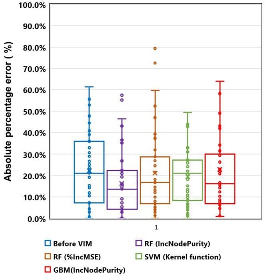
Figure 12.
Boxplot of absolute percentage error for supervised learning models before and after variables importance method (VIM).
Table 4.
Comparison of performance indicators of various supervised learning models.
However, as shown in the boxplot in Figure 12, the problem of reproducibility of the test sets forecast results has been found, and more than 70% of the APE, which has been found to be an outlier, affects the overall accuracy of the model. In contrast, RF (VIM %IncMSE) shows more stable results. Therefore, instead of various supervised learning algorithms, it is recommended that one develops a production forecast model using RF (VIM %IncMSE).
5.2. Comparative Analysis of Re-Training Using Clustering Analysis
In this subsection, we consider examining the influence of datasets categorized with clustering analysis when predicting for shale gas reservoirs. The previous clustering validity analysis calculated an optimal number of clusters, and we re-learned the classified dataset for each cluster and compared and analyzed the model trained by applying RF (VIM IncNodePurity) considered in 5.1 subsecrtion (Figure 13 and Table 5).
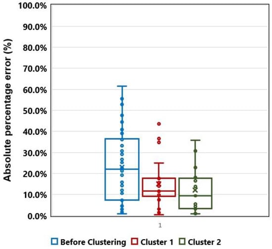
Figure 13.
Boxplot of absolute percentage error for supervised learning models before and after clustering analysis.
Table 5.
Comparison of performance indicators of before and after clustering analysis.
The cluster 1 model had a MAD of 0.180 Bcf, RMSE of 0.224 and MAPE of 14.94%, and R2 of 0.74, respectively. A similar trend and results were found for the cluster 2 model, with a MAD of 0.154 Bcf, RMSE of 0.209 and MAPE of 12.05%, R2 of 0.88, respectively. Among them, the predicted performance of the two cluster models was found to be particularly higher. From the above results, re-training for finding similarities in datasets through cluster analysis can improve the predictive model.
6. Conclusions
The method of productivity forecasting in unconventional reservoirs should be applied different from the conventional reservoirs. It is associated with hydraulic fracturing, well completion, and various well information. This study introduced a robust model and workflow of productivity prediction using machine learning for shale reservoirs at the early time stages of less than 6 months. Data-preprocessing was performed with data from 150 shale gas wells in Eagle Ford shale, Texas. The 129 shale gas wells for data-preprocessing were used as training datasets for supervised learning models.
The emphasis in this study is to generate a more accurate and robust model. First, the importance of variables was evaluated when constructing the predictive model using the RF regression analysis based on VIM. As a result, %IncMSE, IncNodePurity were estimated as the highest variables: Qi_3M, Slickwater, PeakBOE, TVD, THP, Laterallength, and Prop. The predictive performance of the supervised learning model, including RF, SVM, and GBM was evaluated before and when VIM applied. It showed that the RF model with the IncNodePurity based VIM has the highest accuracy compared to other models. Finally, after grouping datasets through cluster analysis, comparing the predictive performance before and after the clustering analysis. Both models of the clustering analysis (cluster 1, 2 model) were found to be more accurate than the original models before the clustering analysis.
In this study, developed model and workflow have been validated in Eagle Ford shale reservoirs. Nevertheless, this research is just a discovery that may be valid in the Eagle Ford shale formation. It is also a forecasting model that can be used in the initial production time (less than 6-months). However, further research will be conducted to overcome these limitations and verify the reliability of the developed model. We will use the data from another shale reservoirs to train and validate the predictive model. Then, the forecasting model will be developed with available data from characteristics of shale gas development prior to in-situ. In addition, only numerical variables were used in this study. The availability of the categorical variable model will be evaluated in the future research.
Author Contributions
D.H. and S.K. designed research, J.J. coordinated investigation and data analysis; D.H. completed the machine learning modeling and statistical analysis and wrote the manuscript. All authors have read and agreed to the published version of the manuscript.
Funding
This work was supported by the Korea Institute of Energy Technology Evaluation and Planning (KETEP) granted financial resource from the Ministry of Trade, Industry & Energy, Republic of Korea (No. 20182510102500).
Conflicts of Interest
The authors declare no conflict of interest.
References
- U.S. Energy Information Administration. Shale Gas Production Includes Associated Natural Gas from Tight Oil Plays 2018. 2018. Available online: https://www.eia.gov/outlooks/aeo/pdf/AEO2018.pdf (accessed on 1 January 2020).
- Wilson, K.C.; Durlofsky, L.J. Optimization of shale gas field development using direct search techniques and reduced-physics models. J. Pet. Sci. Eng. 2013, 108, 304–315. [Google Scholar] [CrossRef]
- Ibrahim, M.; Wattenbarger, R.A. Analysis of rate dependence in transient linear flow in tight gas wells. In Proceedings of the 2006 Abu Dhabi International Petroleum Exhibition and Conference, Abu Dhabi, UAE, 5–8 November 2006. [Google Scholar] [CrossRef]
- Nobakht, M.; Clarkson, C.R. A new analytical method for analyzing production data from tight/shale gas reservoirs exhibiting linear flow: Constant pressure boundary-condition. SPE Res. Eval. Eng. 2012, 15, 370–384. [Google Scholar] [CrossRef]
- Clarkson, C.R.; Qanbari, F. An approximate semi-analytical multiphase forecasting method for multifractured tight light-oil wells with complex fracture geometry. J. Can. Pet. Technol. 2015, 54, 489–508. [Google Scholar] [CrossRef]
- Behmanesh, H.; Hamdi, H.; Clarkson, C.R. Production data analysis of liquid rich shale gas condensate reservoirs. J. Nat. Gas Sci. Eng. 2015, 22, 22–34. [Google Scholar] [CrossRef]
- Clarkson, C.R.; Haghshenas, B.; Ghanizadeh, A.; Qanbari, F.; Williams-Kovacs, J.D.; Riazi, N.; Debuhr, C.; Deglint, H.J. Nanopores to megafractures: Current challenges and methods for shale gas reservoir and hydraulic fracture characterization. J. Nat. Gas Sci. Eng. 2016, 31, 612–657. [Google Scholar] [CrossRef]
- Anderson, D.M.; Nobakht, M.; Mohadam, S.; Mattar, L. Analysis of Production Data from Fractured Shale Gas Wells. In Proceedings of the SPE Unconventional Gas Conference, Pittsburgh, PA, USA, 23–25 February 2010. [Google Scholar]
- Arps, J.J. Analysis of Decline Curves. Trans. AIME 1945, 160, 228–247. [Google Scholar] [CrossRef]
- Ilk, D.; Rushing, J.A.; Perego, A.D.; Blasingame, T.A. Exponential vs. Hyperbolic decline in tight gas sands: Understanding the origin and implications for reserve estimates using arps decline curves. In Proceedings of the SPE Annual Technical Conference and Exhibition, Denver, CO, USA, 21–24 September 2008. [Google Scholar]
- Kupchnenko, C.L.; Gault, B.W.; Mattar, L. Tight Gas Production Performance Using Decline Curves. In Proceedings of the CIPC/SPE Gas Technology Symposium Joint Conference, Calgary, AB, Canada, 16–19 June 2008. [Google Scholar]
- Valkó, P.P.; Lee, J.W. A better way to forecast production from unconventional gas wells. In Proceedings of the SPE Annual Technical Conference and Exhibition, Florence, Italy, 19–22 September 2010. [Google Scholar]
- Duong, A.N. Rate-decline analysis for fracture-dominated shale reservoirs. SPE Reserv. Eval. Eng. 2011, 14, 377–387. [Google Scholar] [CrossRef]
- Clark, A.J.; Lake, L.W.; Patzek, T.W. Production forecasting with logistic growth models. In Proceedings of the SPE Annual Technical Conference and Exhibition, Denver, CO, USA, 30 October–2 November 2011. [Google Scholar]
- Han, D.; Kwon, S. Selection of decline curve analysis method using the cumulative production in cline rate for transient production data obtained from a multi-stage hydraulic fractured horizontal well in unconventional gas fields. Int. J. Oil Gas Coal Technol. 2018, 18, 384–401. [Google Scholar] [CrossRef]
- Mohaghegh, S.D. Reservoir Modeling of Shale Formations. J. Nat. Gas Sci. Eng. 2013, 12, 22–33. [Google Scholar] [CrossRef]
- Zhong, M.; Schuetter, J.; Mishra, S.; Lafollette, R.F. Do data mining methods matter? A Wolfcamp Shale case study. In Proceedings of the SPE Hydraulic Fracturing Technology Conference and Exhibition, The Woodlands, TX, USA, 3–5 February 2015. [Google Scholar]
- Sfidari, E.; Kadkhodaie-Ilkhchi, A.; Najjari, S. Comparison of intelligent and statistical clustering approaches to predicting total organic carbon using intelligent systems. J. Pet. Sci. Eng. 2012, 86–87, 190–205. [Google Scholar] [CrossRef]
- Jung, H.; Jo, H.; Kim, S.; Lee, K.; Choe, J. Geological model sampling using PCA-assisted support vector machine for reliable channel reservoir characterization. J. Pet. Sci. Eng. 2018, 167, 396–405. [Google Scholar] [CrossRef]
- Bansal, Y.; Ertekin, T.; Karpyn, Z.; Ayala, L.; Nejad, A.; Suleen, F.; Balogun, O.; Sun, Q. Forecasting well performance in a discontinuous tight oil reservoirs using artificial neural networks. In Proceedings of the SPE Unconventional Resources Conference, The Woodlands, TX, USA, 10–12 April 2013. [Google Scholar]
- Lolon, E.; Hamidieh, K.; Weijers, L.; Mayerhofer, M.; Melcher, H.; Oduba, O. Evaluating the Relationship Between Well Parameters and Production Using Multivariate Statistical Models: A Middle Bakken and Three Forks Case History. In Proceedings of the SPE Hydraulic Fracturing Technology Conference, The Woodlands, TX, USA, 9–11 February 2016. [Google Scholar]
- Alabboodi, M.J.; Mohaghegh, S.D. Conditioning the Estimating Ultimate Recovery of Shale Wells to Reservoir and Completion Parameters. In Proceedings of the SPE Eastern Regional Meeting, Canton, OH, USA, 13–15 September 2016. [Google Scholar]
- Mohaghegh, S.D.; Gaskari, R.; Maysami, M. Shale Analytics: Making Production and Operational Decisions Based on Facts: A Case Study in Marcellus Shale. In Proceedings of the SPE Hydraulic Fracturing Technology Conference, The Woodlands, TX, USA, 24–26 January 2017. [Google Scholar]
- Li, Y.; Han, Y. Decline Curve Analysis for Production Forecasting Based on Machine Learning. In Proceedings of the SPE Symposium: Production Enhancement and Cost Optimization, Kuala Lumpur, Malaysia, 7–8 November 2017. [Google Scholar]
- Breiman, L. Bagging predictors. Mach. Learn. 1996, 24, 123–140. [Google Scholar] [CrossRef]
- Freund, Y.; Schapire, R.E. A Decision-Theoretic Generalization of On-Line Learning and an Application to Boosting. J. Comput. Syst. Sci. 1997, 55, 119–139. [Google Scholar] [CrossRef]
- Friedman, J.; Hastie, T.; Tibshirani, R. Additive logistic regression: A statistical view of boosting (With discussion and a rejoinder by the authors). Ann. Stat. 2000, 28, 337–407. [Google Scholar] [CrossRef]
- Friedman, J.H. Greedy Function Approximation: A Gradient Boosting Machine. Ann. Stat. 2001, 29, 1189–1232. [Google Scholar] [CrossRef]
- Cortes, C.; Vapnik, V. Support vector machine. Mach. Learn. 1995, 20, 273–297. [Google Scholar] [CrossRef]
- Jiang, S.; Mokhtari, M. Characterization of marl and interbedded limestone layers in the Eagle Ford Formation, DeWitt county, Texas. J. Pet. Sci. Eng. 2019, 172, 502–510. [Google Scholar] [CrossRef]
- Wang, M.; Wang, L.; Zhou, W.; Yu, W. Lean gas Huff and Puff process for Eagle Ford Shale: Methane adsorption and gas trapping effects on EOR. Fuel 2019, 248, 143–151. [Google Scholar] [CrossRef]
- Min, B.H.; Min, B.H.; Park, C.H.; Kang, J.M.; Park, H.J.; Jang, I.S. Optimal Well Placement Based on Artificial Neural Network Incorporating the Productivity Potential. Energy Source. Part A 2011, 33, 1726–1738. [Google Scholar] [CrossRef]
- Nguyen, H.; Bui, X.N.; Nguyen-Thoi, T.; Ragam, P.; Moayedi, H. Toward a State-of-the Art of Fly Rock Prediction Technology in Open-Pit Mines Using EANNs Model. Appl. Sci. 2019, 9, 4554. [Google Scholar] [CrossRef]
- Nguyen, T.T.; Yoon, S. A Novel Approach to Short-Term Stock Price Movement Prediction using Transfer Learning. Appl. Sci. 2019, 9, 4745. [Google Scholar] [CrossRef]
- Arora, P.; Deepali; Varshney, S. Analysis of K-Means and K-Medoids Algorithm for Big Data. Procedia Comput. Sci. 2016, 78, 507–512. [Google Scholar] [CrossRef]
© 2020 by the authors. Licensee MDPI, Basel, Switzerland. This article is an open access article distributed under the terms and conditions of the Creative Commons Attribution (CC BY) license (http://creativecommons.org/licenses/by/4.0/).