Article

Reducing Computational Complexity and Memory Usage of Iterative Hologram Optimization Using Scaled Diffraction

1
Graduate School of Engineering, Chiba University, Chiba 263-8522, Japan
2
Faculty of Physics, Warsaw University of Technology, Warsaw 00-662, Poland
3
Faculty of Systems Design, Tokyo Metropolitan University, Tokyo 191-0065, Japan
4
National Institute of Technology, Oyama College, Tochigi 323-0806, Japan
*
Author to whom correspondence should be addressed.
Appl. Sci. 2020, 10(3), 1132; https://doi.org/10.3390/app10031132
Submission received: 19 December 2019 / Revised: 22 January 2020 / Accepted: 27 January 2020 / Published: 7 February 2020
(This article belongs to the Special Issue Practical Computer-Generated Hologram for 3D Display)

Abstract

:
A complex amplitude hologram can reconstruct perfect light waves. However, as there are no spatial light modulators that are able to display complex amplitudes, we need to use amplitude, binary, or phase-only holograms. The images reconstructed from such holograms will deteriorate; to address this problem, iterative hologram optimization algorithms have been proposed. One of the iterative algorithms utilizes a blank area to help converge the optimization; however, the calculation time and memory usage involved increases. In this study, we propose to reduce the computational complexity and memory usage of the iterative optimization using scaled diffraction, which can calculate light propagation with different sampling pitches on a hologram plane and object plane. Scaled diffraction can introduce a virtual blank area without using physical memory. We further propose a combination of scaled diffraction-based optimization and conventional methods. The combination algorithm improves the quality of a reconstructed complex amplitude while accelerating optimization.

1. Introduction

Light waves are essentially represented by complex amplitudes. Therefore, if we can display a complex amplitude hologram on a spatial light modulator (SLM), we can reconstruct perfect light waves. Complex amplitude holograms can be displayed by using two SLMs [1], or by dividing the displaying areas of a single SLM [2,3]. However, in the former, it can be difficult to alight two SLMs precisely, and the latter sacrifices the spatial bandwidth product of an SLM.
As there is no single spatial light modulator that can display complex amplitudes, we must convert the complex amplitude holograms to amplitude, binary, or phase-only holograms [4]. The reconstructed images from such holograms are degraded because of noises. To address this problem, deterministic methods have been proposed to encode to amplitude, binary, or phase-only holograms [5,6,7,8,9]. Although noniterative methods are computationally effective, they decrease the spatial bandwidth product of the SLM because of the use of superpixels and the spatial multiplexing of two holograms.
In addition, iterative optimization algorithms have been proposed [10,11,12,13,14,15]. A representative algorithm is the Gerchberg–Saxton (GS) algorithm [16]. The GS algorithm has a wide range of applications; for example, the measurement of unknown complex-valued objects from diffraction patterns or holograms; vortex beam generation; multi-spot generation; and the optimization of holograms that can display high-quality reconstructed images. We then focus on the hologram optimization for display purposes. The GS algorithm iteratively calculates the light propagation and back-propagation between the object plane and the hologram plane to optimize the hologram. During this iteration, some constraints, based on prior information, are imposed on the hologram plane and object plane. One of the GS-based algorithms uses a blank area to help the convergence of the optimization [10,11,12,14]. However, the calculation time and memory usage increase.
In this study, we propose the reduction of computational complexity and memory usage for iterative optimization using scaled diffraction that can calculate light propagation with different sampling pitches on a hologram plane and object plane. The scaled diffraction can introduce a virtual blank area without using physical memory. We demonstrate that the proposed method can reconstruct a better complex amplitude from an optimized hologram. We further propose an algorithm that combines scaled diffraction-based optimization with conventional methods. The combination algorithm improves the quality of the reconstructed complex amplitude while accelerating iteration optimization.

2. Proposed Method

This section describes the two proposed methods, using scaled diffraction. First, we explain a conventional iterative algorithm [14]. Next, we explain the two proposed methods. The first method uses scaled diffraction and the second method uses the scaled diffraction-based iterative algorithm, followed by the conventional method.

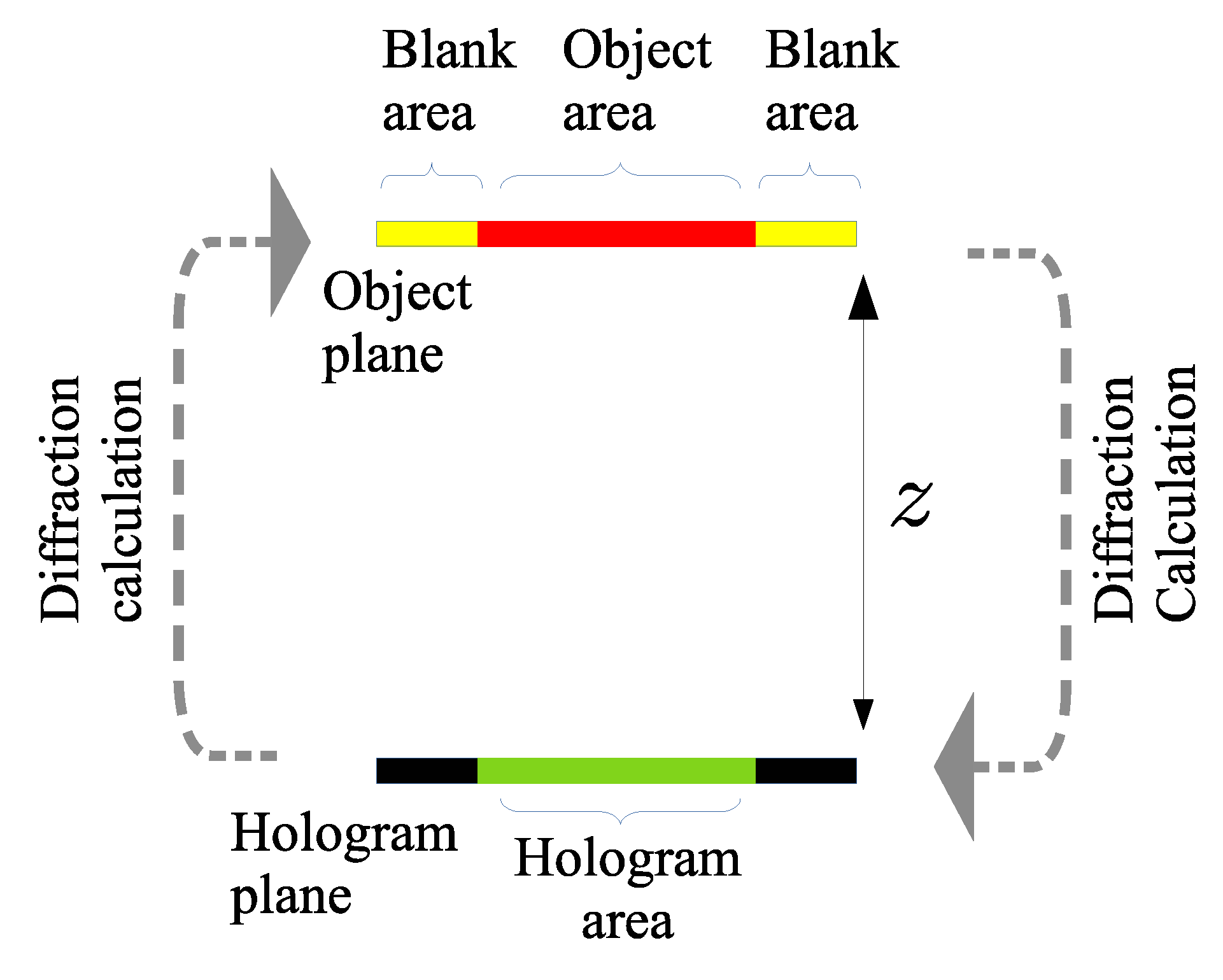
2.1. Conventional Method

A conventional iterative algorithm [14] optimizes a phase-only hologram to reconstruct the desired complex amplitude, in which a blank area is introduced around the original complex amplitude o ( x , y ) . The size of the original complex amplitude is N × N pixels. The expanded object plane u o ( x , y ) with the blank area has m N × m N pixels, where m denotes the magnification of the expansion. The magnification m indicates the ratio between the sizes of the original object plane to the expanded one. The size of the hologram plane u h ( x , y ) is the same as that of u o ( x , y ) .
The flow of the conventional algorithm is shown in Figure 1 and is performed in the following steps:
  • We initially set random phase values in the hologram plane u h ( x , y ) ;
  • We compute the diffraction calculation from u h ( x , y ) to the object plane u o ( x , y ) with the propagation distance + z ;
  • As an object plane constraint, the area where the original object in u o ( x , y ) exists is replaced by o ( x , y ) , while the calculated value in the blank area remains;
  • The updated u o ( x , y ) is back-propagated to the hologram plane u h ( x , y ) by the same diffraction calculation with the propagation distance z ;
  • We introduce two constraints to the hologram plane. The first constraint is to calculate u h ( x , y ) = u h ( x , y ) / | u h ( x , y ) | because our target is a phase-only hologram. The second constraint is the support of the hologram. We set zero values in the blank area of the hologram plane, because the size of the hologram is N × N ;
  • We repeat Steps 2 to 5 until the number of iterations reaches a predefined number, or the image quality of the reconstructed complex amplitude reaches a predefined quality, or the image quality of the reconstructed complex amplitude decreases;
  • To obtain the final hologram, we crop only the central part of u h ( x , y ) with N × N pixels.
The computational complexity of the algorithm is O ( L m 2 N 2 log 2 m N ) , where L is the number of the iterations. Memory usage requires O ( m 2 N 2 ) .

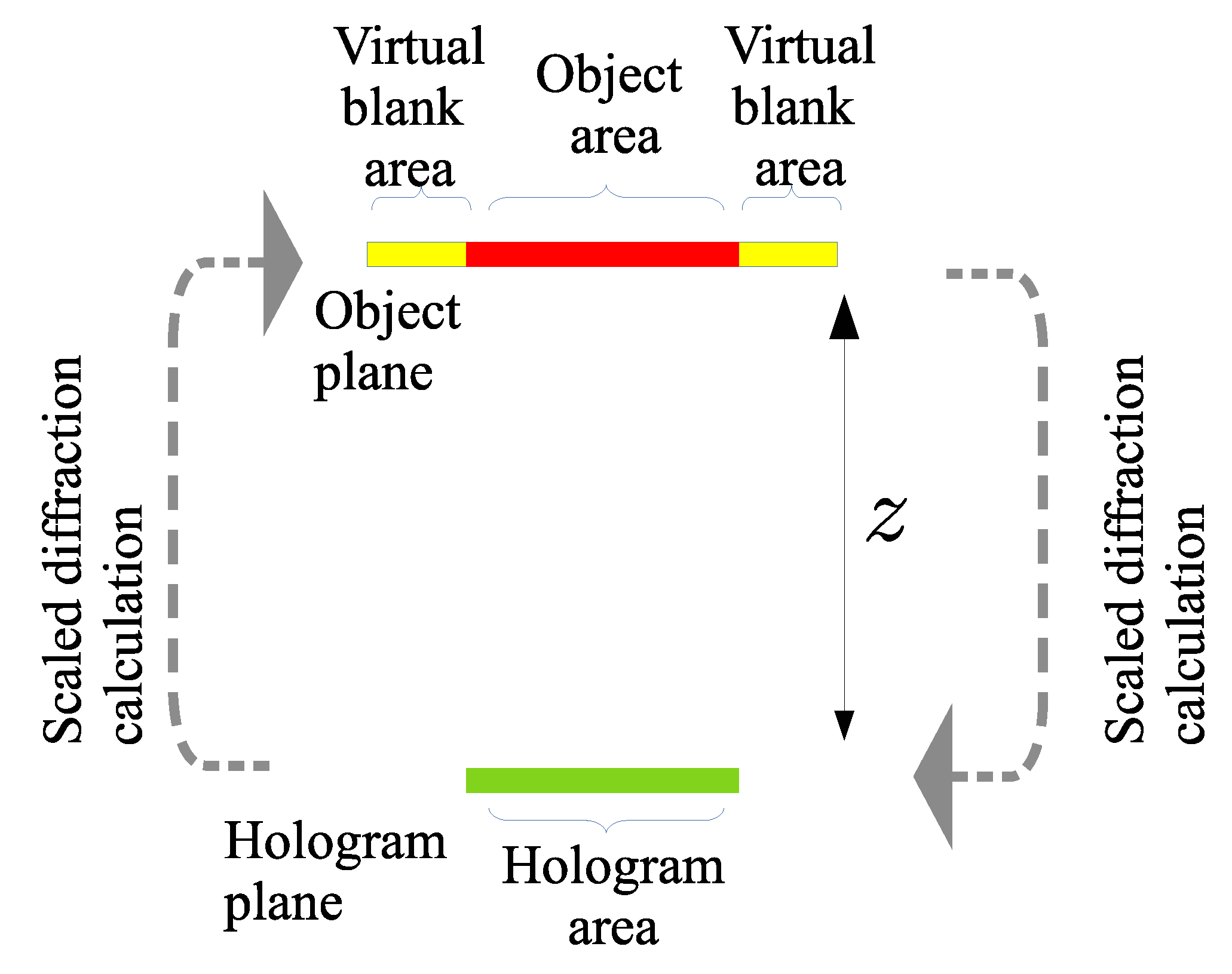
2.2. Proposed Method 1: Scaled Diffraction-Based Hologram Optimization

A conventional algorithm can optimize a hologram. However, by introducing the blank area, it requires an expanded area that is m-times the size of the original hologram. In this section, we describe the proposed algorithm, which uses scaled diffraction to introduce a virtual blank area, to solve this problem. Several scaled diffraction calculations have been previously proposed [17,18,19,20,21,22]. In this study, we used aliasing-reduced shifted and scaled (ARSS)-Fresnel diffraction [22] as the scaled diffraction. The ARSS-Fresnel diffraction can perform Fresnel diffraction with different sampling pitches on the source and destination planes. Note that the number of pixels on the source and destination is N × N pixels. As with other diffraction calculations, the ARSS-Fresnel diffraction can be acceleration using fast Fourier transforms (FFTs). In this study, we denote the operator of the scaled diffraction as
u 2 ( x , y ) = P p 1 , p 2 z { u 1 ( x , y ) } ,
where u 1 ( x , y ) and u 2 ( x , y ) are the source plane and destination plane with sampling pitches p 1 and p 2 , respectively, and z is the distance between the planes. For simplicity, we only show the one-dimensional ARSS-Fresnel diffraction, but two-dimensional ARSS-Fresnel diffraction can be simply derived using separation of variables in Fresnel diffraction. The ARSS-Fresnel diffraction is expressed as
u 2 ( x 2 ) = P p 1 , p 2 z { u 1 } = C z F 1 [ F [ u 1 ( x 1 ) exp ( i ϕ u ) ] F [ exp ( i ϕ h ) Rect ( x h 2 x m a x ) ] ] ,
where x 1 = p 1 m and x 2 = p 2 n , and where N / 2 m , n < N / 2 are the integer coordinates, F · denotes the Fourier transform, Rect ( · ) is the rectangular function for reducing aliasing error, x h is a variable for the generation of exp ( i ϕ h ) , x m a x is the aliasing-free area and exp ( i ϕ u ) , exp ( i ϕ h ) and C z are defined by exp ( i ϕ u ) = exp ( i π ( ( s 2 s ) x 1 2 ) / ( λ z ) ) , exp ( i ϕ h ) = exp ( i π s x h 2 / ( λ z ) ) and C z = exp ( i ϕ c ) / ( i λ z ) = exp ( i k z + i π ( ( 1 s ) x 2 2 ) ) / ( λ z ) ) / ( i λ z ) , where s is defined by p 1 / p 2 .
The flow of the proposed algorithm is shown in Figure 2. The proposed algorithm using the scaled diffraction is performed in the following steps:
  • We initially set random phase values in the hologram plane u h ( x , y ) , with the sampling pitch p h ;
  • We compute the diffraction calculation from u h ( x , y ) to the object plane u o ( x , y ) with the sampling pitch of p o = m p h where m is the magnification. The calculation is performed by
    u o ( x , y ) = P p h , p o z { u h ( x , y ) } ;
  • As an object plane constraint, the area where the original object in the object plane exists is replaced by down-sampled original object o d ( x , y ) with the number of pixels N / m × N / m . The complex values in the virtual blank area remain;
  • The updated u o ( x , y ) is back-propagated to the hologram plane u h ( x , y ) using the same diffraction calculation:
    u h ( x , y ) = P p o , p h z { u o ( x , y ) } ;
  • As a constraint on the hologram plane, we calculate u h ( x , y ) = u h ( x , y ) / | u h ( x , y ) | , because our target is a phase-only hologram;
  • We repeat Steps 2 to 5 until the number of iterations reaches a predefined number or the image quality of the reconstructed complex amplitude reaches a predefined quality.
We used scaled diffraction in Steps 2 and 4. The number of pixels in the scaled diffraction source and destination planes is N × N , unlike in the case of the conventional algorithm; therefore, the computational complexity and memory usage of the algorithm are only O ( L N 2 log 2 N ) and O ( N 2 ) , respectively. We can reduce the computational complexity and memory usage of the conventional algorithm by a factor of 1 / m 2 .

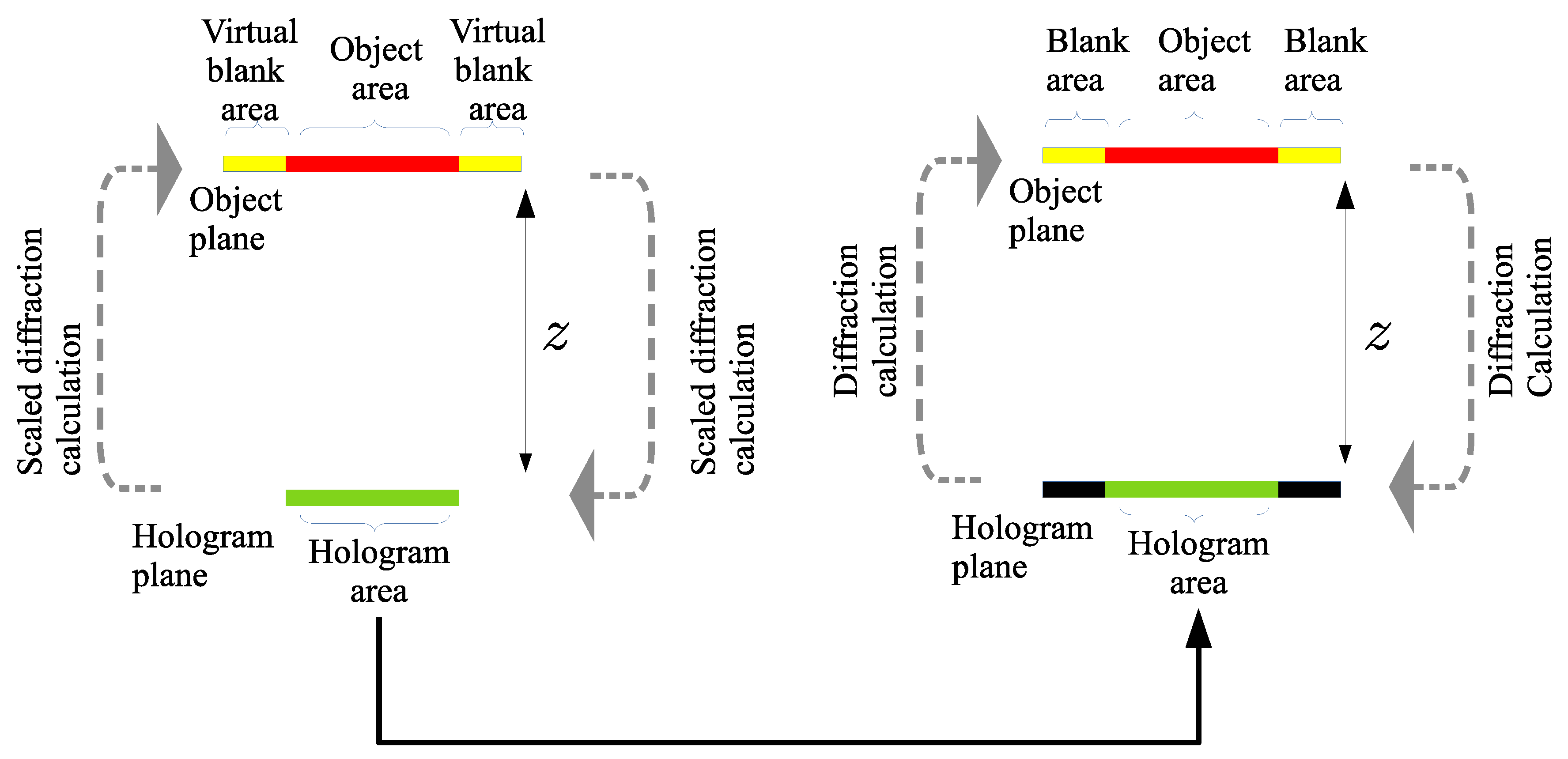
2.3. Proposed Method 2: Combination Algorithm
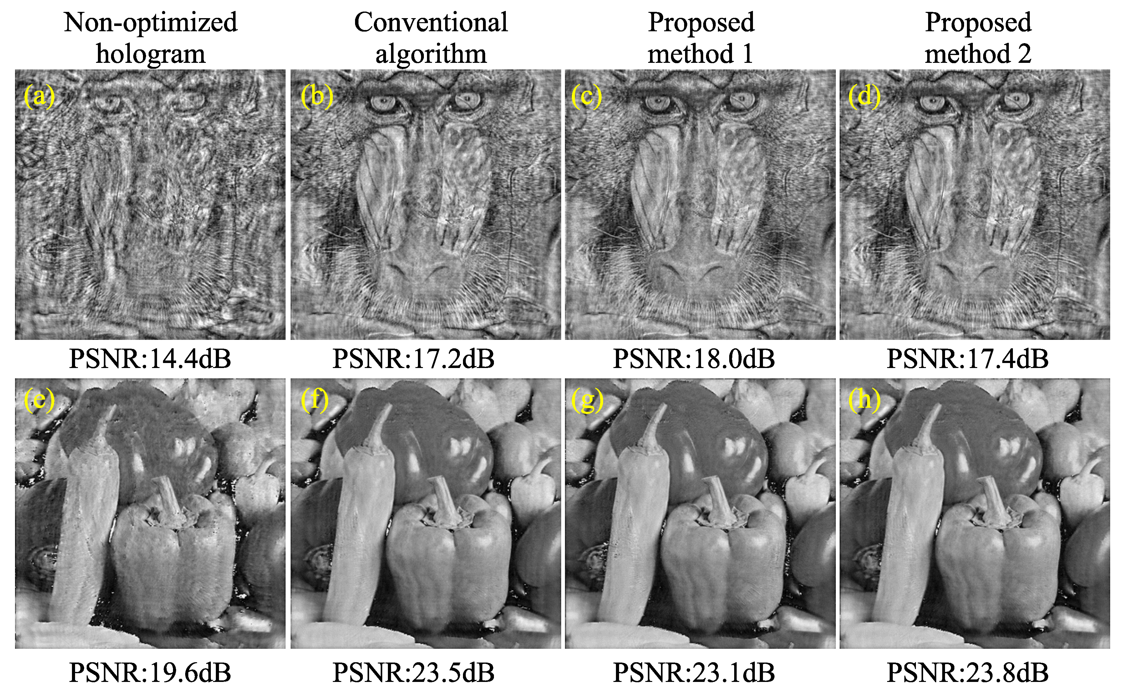
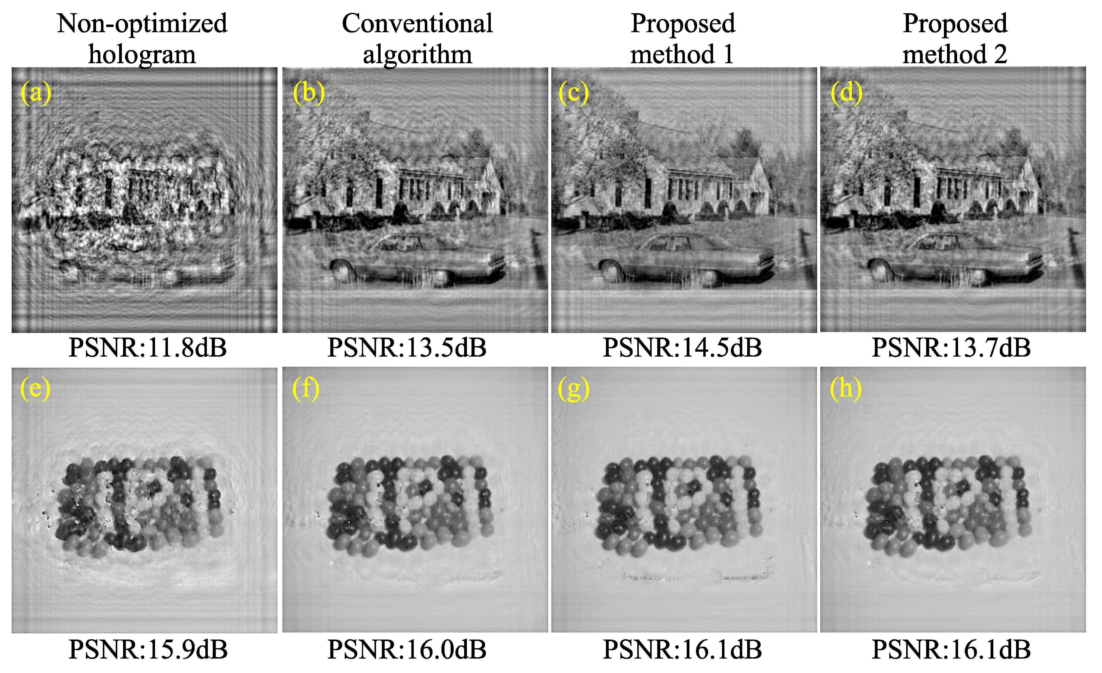
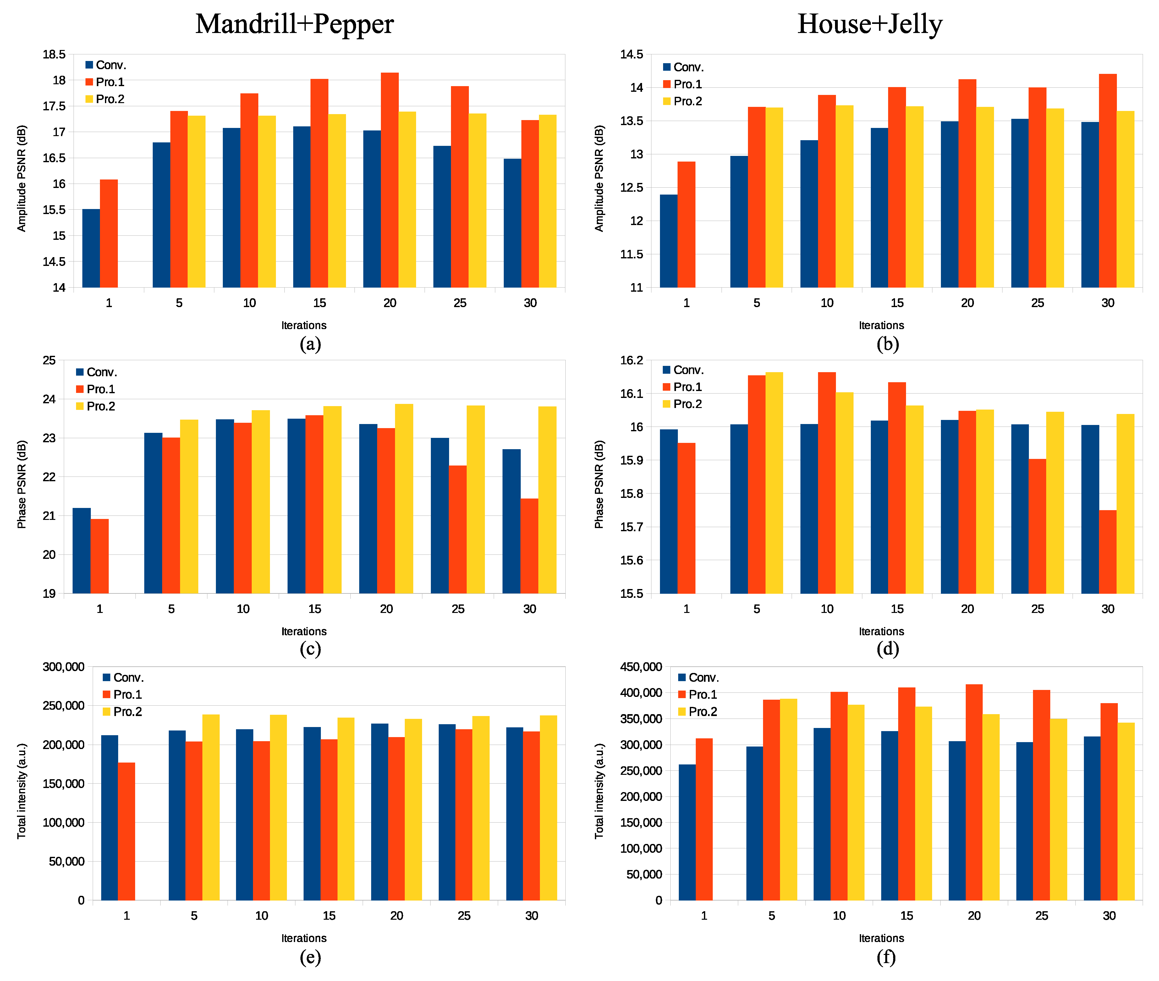
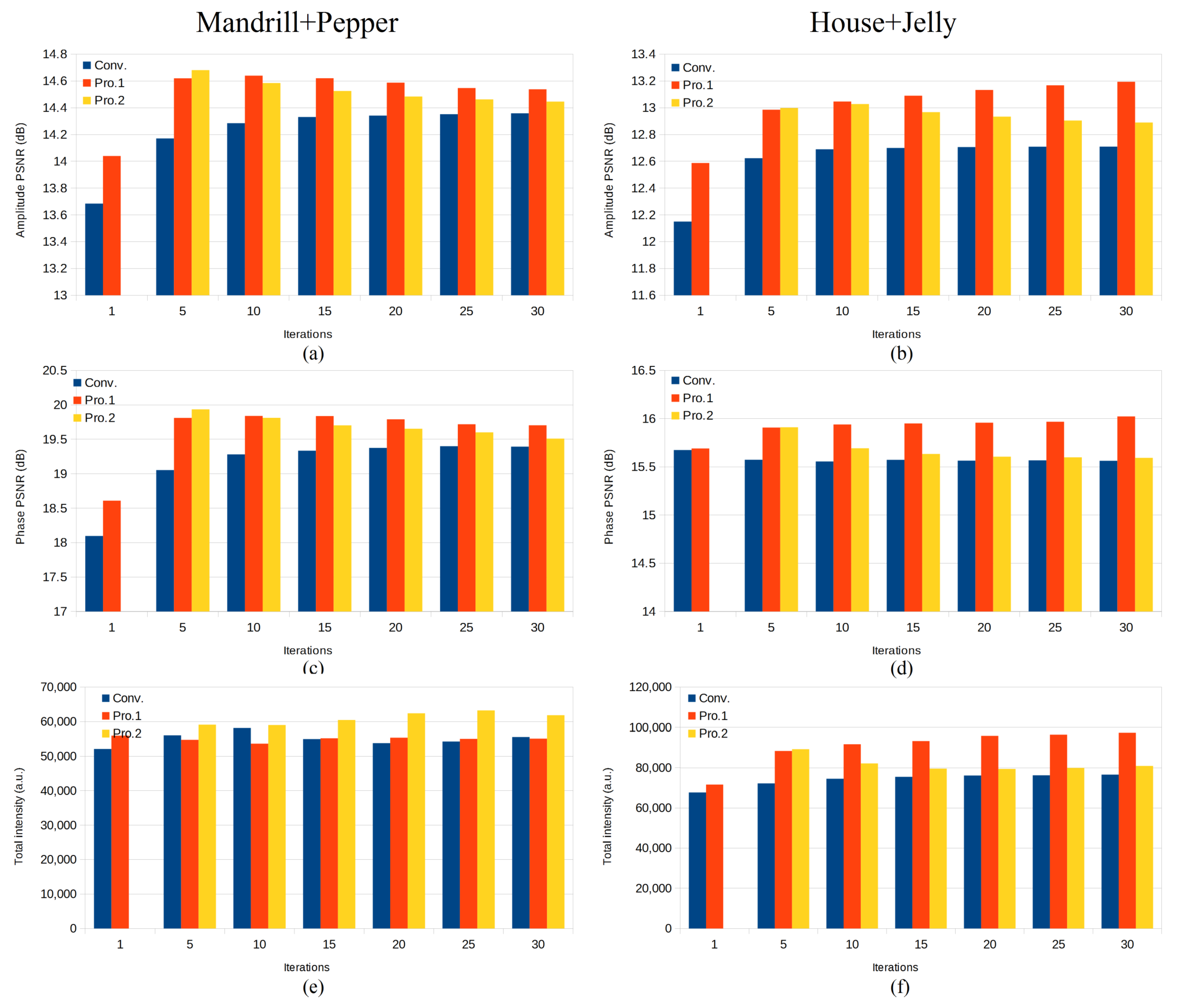
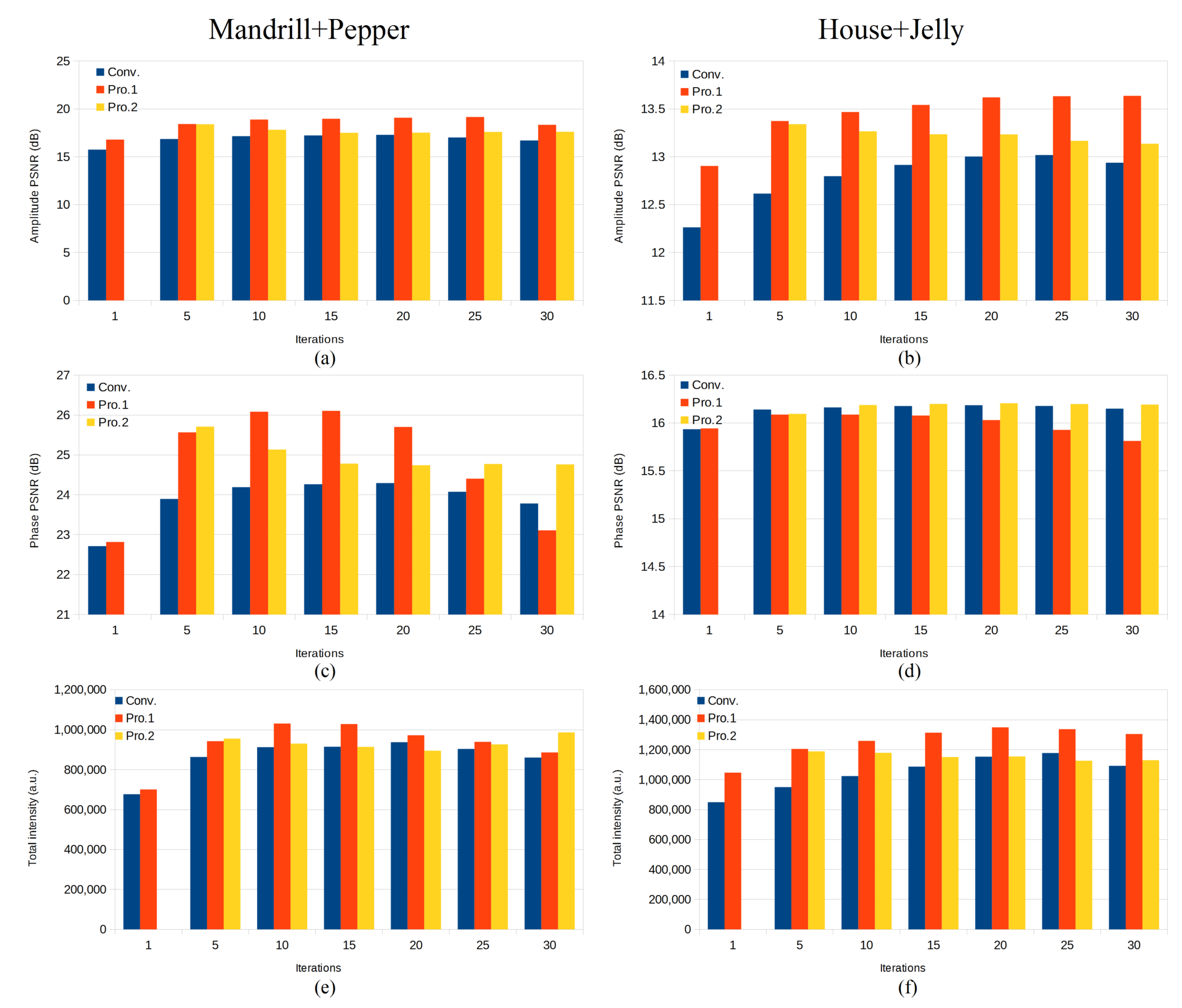
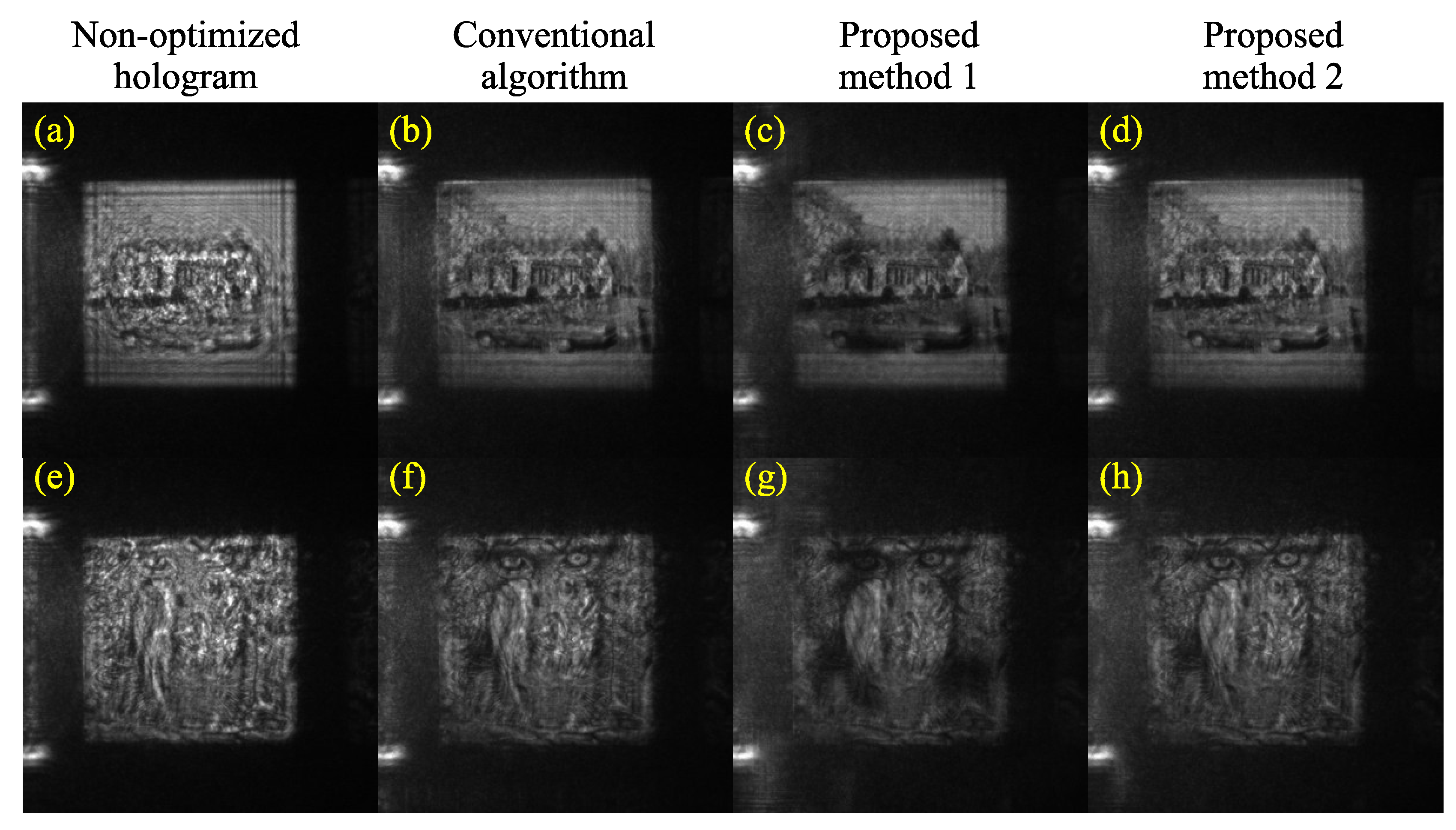
The second proposed method is a combination of a scaled diffraction-based algorithm (described in Section 2.2) and a conventional algorithm (described in Section 2.1). In some cases, the results of scaled diffraction-based algorithms are inferior to those of conventional algorithms. While maintaining the advantage (low computational complexity) of scaled diffraction-based algorithms, we improve this problem by combining a scaled diffraction-based algorithm with a conventional algorithm. Figure 3 shows the flow of the combination algorithm.
First, the hologram is optimized by a scaled diffraction-based algorithm with the iteration number L 1 . The hologram is then further optimized by a conventional algorithm with the iteration number L 2 . The total computational complexity and memory usage of the combination algorithm are only O ( L 1 N 2 log 2 N + L 2 m 2 N 2 log 2 m N ) and O ( m 2 N 2 ) , respectively.

3. Results

We have discussed reconstructed complex amplitudes obtained from a non-optimized phase-only hologram, optimized holograms using the conventional algorithm, a scaled diffraction-based algorithm (Proposed method 1), and a combination algorithm (Proposed method 2). Non-optimized phase-only holograms are calculated by simply propagating the object plane using a Fresnel diffraction calculation. The calculation conditions are a wavelength of 532 nm, z = 0.3 m and the pixel pitch of the hologram p h = 8 μ m. All the calculations were performed using our wave optics library, CWO++ [23]. We used two original objects with complex amplitudes. The first complex-valued object consisted of Mandrill and Pepper images as amplitude and phase, respectively. The second complex-valued object consisted of House and Jelly images as amplitude and phase, respectively.
Figure 4 shows the reconstructed amplitude images (upper row) and phase images (bottom row) obtained from a non-optimized hologram and optimized holograms, respectively. The resolution of the holograms is 1024 × 1024 pixels. The number of iterations in each iterative algorithm is fixed to L = 20 . Note that the combination algorithm used the first and second iteration numbers of L 1 = 0.8 L and L 2 = 0.2 L . We empirically determined the ratio between L 1 and L 2 . If L 2 is large, the effect of improving the image quality cannot be expected to be substantial, and only the calculation time increases. We measured the quality of the reconstructed amplitude and phase images using the peak signal-to-noise ratio (PSNR) between the original and reconstructed images. In the reconstructed amplitude image, the proposed methods can reconstruct better images than the conventional method. In particular, Proposed method 1 had the highest quality. In the reconstructed phase image, Proposed method 1 was slightly inferior to the other methods. In contrast, Proposed method 2 had the highest quality of the reconstructed phase images. The calculation times for the conventional algorithm, Proposed method 1, and Proposed method 2 were 58 s, 15 s, and 23 s, respectively. Proposed methods 1 and 2 can accelerate hologram optimization approximately 4 times and 2.5 times faster, respectively, than the conventional algorithm.
The difference between the conventional method and the proposed methods is the use of scaled diffraction. The sampling pitch on the object plane in the scaled diffraction is larger than that of the conventional diffraction calculation, leading to the averaging effect of noises on the object plane. The averaging effect gradually reduces the noise in the reconstructed images during the iterations of the proposed methods.
Figure 5 shows the reconstructed amplitude images (upper row) and phase images (bottom row) obtained from a non-optimized hologram and optimized holograms, respectively. The calculation conditions were the same as those in Figure 4. In this case, the two proposed methods have better quality outcomes than the conventional algorithm. Proposed methods 1 and 2 can also accelerate hologram optimization by approximately 4 times and 2.5 times, respectively, than the conventional algorithm. In particular, the amplitude and phase are the highest in Proposed method 1.
Figure 6 shows the amplitude images, phase images, and total intensity as a function of the iterations. The left and right columns show the results of the original objects “Mandrill+Pepper” and “House+Jelly,” respectively. In the graphs, “Conv,” “Pro1,” and “Pro2” denote the conventional algorithm, Proposed method 1, and Proposed method 2, respectively. In the combination algorithm, the iteration numbers of the first and second optimization were L 1 = 0.8 L and L 2 = 0.2 L , respectively. Note that we did not perform Proposed method 2 in the L = 1 iteration.
Regarding the quality of the reconstructed amplitude images of “Mandrill+Pepper” and “House+Jelly,” Proposed method 1 has a higher quality than the other methods. In contrast, as shown in Figure 6c, the quality of the phase image using Proposed method 1 is no better than the conventional algorithm, but Proposed method 2 maintains the best quality of all the iterations when compared with the other methods. Figure 6e,f show the total intensity of the reconstructed images. The total intensity is defined as the total light intensity of the reconstructed image calculated by x , y | a ( x , y ) | 2 , where a ( x , y ) is the amplitude in the object plane. In Figure 6e, Proposed method 2 has the highest total intensity of all the iterations. In Figure 6f, Proposed method 1 has the highest optical efficiency of all the iterations.
Figure 7 and Figure 8 show the amplitude images, phase images, and total intensity as a function of the iterations. The calculation conditions are the same as in Figure 6, except for the resolution of the holograms. The resolutions of the holograms in Figure 7 and Figure 8 are 512 × 512 pixels and 2048 × 2048 pixels, respectively. Overall, the proposed methods demonstrated better image quality and total intensity than the conventional method.
Figure 9 shows optical reconstructions from holograms with 1024 × 1024 pixels, using the original complex-valued objects of “House+Jelly” and “Mandrill+Pepper.” We used a phase-modulated spatial light modulator with a full high definition (HD) resolution. The calculation condition of the holograms is the same as in Figure 6. Figure 9a,e show the optical reconstructions using the non-iterative method. Figure 9b,f show the optical reconstructions using the conventional method. Figure 9c,g show the optical reconstructions using Proposed method 1 and Figure 9d,h show the optical reconstructions using Proposed method 2. The proposed methods improve the image quality compared to the non-iterative method while reducing the calculation time.

4. Conclusions

We proposed a scaled diffraction-based algorithm for hologram optimization. To introduce the virtual blank area without using physical memory, the scaled diffraction-based algorithm is effective in terms of computational complexity and memory usage, while maintaining the image quality of the reconstructed complex amplitude. However, in some calculation conditions, the quality of the reconstructed complex amplitude obtained from the scaled diffraction-based algorithm was slightly inferior to the conventional algorithm. We further proposed the combination of a scaled diffraction base with conventional algorithms. The computational complexity of this algorithm was less than that of the conventional method, and the image quality, which exceeded the conventional method, could be stably obtained.

Author Contributions

Conceptualization, T.S.; methodology, T.S.; software, T.S., M.M. and T.T.; validation, T.S., M.M. and Y.Y., I.H. and T.N.; formal analysis, T.S.; investigation, T.S.; resources, T.S.; data curation, T.S.; discussion, T.S., M.M., T.T., Y.Y., I.H., T.N., N.H., T.K., T.I.; writing–original draft preparation, T.S.; writing–review and editing, T.S., M.M., T.T., Y.Y., I.H., T.N., N.H., T.K., T.I.; visualization, T.S., M.M.; supervision, T.S.; project administration, T.S.; funding acquisition, T.S. and T.I. All authors have read and agreed to the published version of the manuscript.

Funding

This research was partially funded by JSPS KAKENHI Grant Numbers 19H04132 and 19H01097.

Conflicts of Interest

The authors declare no conflict of interest.

References

  1. Makowski, M.; Siemion, A.; Ducin, I.; Kakarenko, K.; Sypek, M.; Siemion, A.M.; Suszek, J.; Wojnowski, D.; Jaroszewicz, Z.; Kolodziejczyk, A. Complex light modulation for lensless image projection. Chin. Opt. Lett. 2011, 9, 120008. [Google Scholar] [CrossRef] [Green Version]
  2. Liu, J.P.; Hsieh, W.Y.; Poon, T.C.; Tsang, P. Complex Fresnel hologram display using a single SLM. Appl. Opt. 2011, 50, H128–H135. [Google Scholar] [CrossRef] [Green Version]
  3. Rincon, I.; Arrizon, V. Generation of complex optical fields by double phase modulation in a SLM. OSA Contin. 2019, 2, 2983–2996. [Google Scholar] [CrossRef]
  4. Shimobaba, T.; Ito, T. Computer Holography: Acceleration Algorithms and Hardware Implementations; CRC Press: Boca Raton, FL, USA, 2019. [Google Scholar]
  5. Davis, J.A.; Cottrell, D.M.; Campos, J.; Yzuel, M.J.; Moreno, I. Encoding amplitude information onto phase-only filters. Appl. Opt. 1999, 38, 5004–5013. [Google Scholar] [CrossRef]
  6. Mendoza-Yero, O.; Mínguez-Vega, G.; Lancis, J. Encoding complex fields by using a phase-only optical element. Opt. Lett. 2014, 39, 1740–1743. [Google Scholar] [CrossRef] [Green Version]
  7. Goorden, S.A.; Bertolotti, J.; Mosk, A.P. Superpixel-based spatial amplitude and phase modulation using a digital micromirror device. Opt. Express 2014, 22, 17999–18009. [Google Scholar] [CrossRef] [Green Version]
  8. Kong, D.; Cao, L.; Jin, G.; Javidi, B. Three-dimensional scene encryption and display based on computer-generated holograms. Appl. Opt. 2016, 55, 8296–8300. [Google Scholar] [CrossRef]
  9. Shimobaba, T.; Takahashi, T.; Yamamoto, Y.; Hoshi, I.; Shiraki, A.; Kakue, T.; Ito, T. Simple complex amplitude encoding of a phase-only hologram using binarized amplitude. arXiv 2019, arXiv:1909.08177. [Google Scholar]
  10. Akahori, H. Spectrum leveling by an iterative algorithm with a dummy area for synthesizing the kinoform. Appl. Opt. 1986, 25, 802–811. [Google Scholar] [CrossRef]
  11. Wyrowski, F. Diffractive optical elements: Iterative calculation of quantized, blazed phase structures. JOSA A 1990, 7, 961–969. [Google Scholar] [CrossRef]
  12. Georgiou, A.; Christmas, J.; Collings, N.; Moore, J.; Crossland, W.A. Aspects of hologram calculation for video frames. J. Opt. A Pure Appl. Opt. 2008, 10, 035302. [Google Scholar] [CrossRef]
  13. Wu, L.; Cheng, S.; Tao, S. Complex amplitudes reconstructed in multiple output planes with a phase-only hologram. J. Opt. 2015, 17, 125603. [Google Scholar] [CrossRef]
  14. Tao, S.; Yu, W. Beam shaping of complex amplitude with separate constraints on the output beam. Opt. Express 2015, 23, 1052–1062. [Google Scholar] [CrossRef]
  15. Wang, H.; Yue, W.; Song, Q.; Liu, J.; Situ, G. A hybrid Gerchberg–Saxton-like algorithm for DOE and CGH calculation. Opt. Lasers Eng. 2017, 89, 109–115. [Google Scholar] [CrossRef] [Green Version]
  16. Gerchberg, R.W.; Saxton, W.O. A practical algorithm for the determination of phase from image and diffraction plane pictures. Optik 1972, 35, 237–246. [Google Scholar]
  17. Ferraro, P.; De Nicola, S.; Coppola, G.; Finizio, A.; Alfieri, D.; Pierattini, G. Controlling image size as a function of distance and wavelength in Fresnel-transform reconstruction of digital holograms. Opt. Lett. 2004, 29, 854–856. [Google Scholar] [CrossRef]
  18. Muffoletto, R.P.; Tyler, J.M.; Tohline, J.E. Shifted Fresnel diffraction for computational holography. Opt. Express 2007, 15, 5631–5640. [Google Scholar] [CrossRef]
  19. Paturzo, M.; Memmolo, P.; Finizio, A.; Näsänen, R.; Naughton, T.J.; Ferraro, P. Synthesis and display of dynamic holographic 3D scenes with real-world objects. Opt. Express 2010, 18, 8806–8815. [Google Scholar] [CrossRef] [Green Version]
  20. Restrepo, J.F.; Garcia-Sucerquia, J. Magnified reconstruction of digitally recorded holograms by Fresnel–Bluestein transform. Appl. Opt. 2010, 49, 6430–6435. [Google Scholar] [CrossRef]
  21. Odate, S.; Koike, C.; Toba, H.; Koike, T.; Sugaya, A.; Sugisaki, K.; Otaki, K.; Uchikawa, K. Angular spectrum calculations for arbitrary focal length with a scaled convolution. Opt. Express 2011, 19, 14268–14276. [Google Scholar] [CrossRef]
  22. Shimobaba, T.; Kakue, T.; Okada, N.; Oikawa, M.; Yamaguchi, Y.; Ito, T. Aliasing-reduced Fresnel diffraction with scale and shift operations. J. Opt. 2013, 15, 075405. [Google Scholar] [CrossRef] [Green Version]
  23. Shimobaba, T.; Weng, J.; Sakurai, T.; Okada, N.; Nishitsuji, T.; Takada, N.; Shiraki, A.; Masuda, N.; Ito, T. Computational wave optics library for C++: CWO++ library. Comput. Phys. Commun. 2012, 183, 1124–1138. [Google Scholar] [CrossRef] [Green Version]
Figure 1. Conventional algorithm.
Applsci 10 01132 g001
Figure 2. Scaled diffraction-based algorithm.
Applsci 10 01132 g002
Figure 3. Combination algorithm.
Applsci 10 01132 g003
Figure 4. Reconstructed amplitude images (upper row) and phase images (bottom row) obtained from non-optimized hologram and optimized holograms, respectively.
Applsci 10 01132 g004
Figure 5. Reconstructed amplitude images (upper row) and phase images (bottom row) obtained from a non-optimized hologram and optimized holograms, respectively
Applsci 10 01132 g005
Figure 6. Reconstructed amplitude images, phase images, and total intensity as a function of the iterations. The resolution of the hologram is 1024 × 1024 pixels. The peak signal-to-noise ratios (PSNRs) and total intensities were averaged with five different initial random phases. (a,b) are the amplitude PSNRs for “Mandrill+Pepper” and “House+Jelly”, (c,d) the phase PSNRs for “Mandrill+Pepper” and “House+Jelly”, and (e,f) are the total intensities for “Mandrill+Pepper” and “House+Jelly.”
Applsci 10 01132 g006
Figure 7. Reconstructed amplitude images, phase images, and total intensity as a function of the iterations. The resolution of the hologram is 512 × 512 pixels. (a,b) are the amplitude PSNRs for “Mandrill+Pepper” and “House+Jelly”, (c,d) the phase PSNRs for “Mandrill+Pepper” and “House+Jelly”, and (e,f) are the total intensities for “Mandrill+Pepper” and “House+Jelly.”
Applsci 10 01132 g007
Figure 8. Reconstructed amplitude images, phase images, and total intensity as a function of the iterations. The resolution of the hologram is 2048 × 2048 pixels. (a,b) are the amplitude PSNRs for “Mandrill+Pepper” and “House+Jelly”, (c,d) the phase PSNRs for “Mandrill+Pepper” and “House+Jelly”, and (e,f) are the total intensities for “Mandrill+Pepper” and “House+Jelly.”
Applsci 10 01132 g008
Figure 9. Optical reconstructions from holograms with 1024 × 1024 pixels: (a,e) show reconstructed images obtained from the non-optimized hologram, (b,f) show reconstructed images obtained from the conventional algorithm, (c,g) show reconstructed images obtained from the proposed method 1, and (d,h) show reconstructed images obtained from the proposed method 2.
Applsci 10 01132 g009

