Theoretical Analysis of Fractional Viscoelastic Flow in Circular Pipes: General Solutions

Abstract

Fractional calculus is a relatively old yet emerging field of mathematics with the widest range of engineering and biomedical applications. Despite being an incredibly powerful tool, it, however, requires promotion in the engineering community. Rheology is undoubtedly one of the fields where fractional calculus has become an integral part of cutting-edge research. There exists extensive literature on the theoretical, experimental, and numerical treatment of various fractional viscoelastic flows in constraint geometries. However, the general theoretical approach that unites several most commonly used models is missing. Here we present exact analytical solutions for fractional viscoelastic flow in a circular pipe. We find velocity profiles and shear stresses for fractional Maxwell, Kelvin–Voigt, Zener, Poynting–Thomson, and Burgers models. The dynamics of these quantities are studied with respect to normalized pipe radius, fractional orders, and elastic moduli ratio. Three different types of behavior are identified: monotonic increase, resonant, and aperiodic oscillations. The models developed are applicable in the widest material range and allow for the alteration of the balance between viscous and elastic properties of the materials.

1. Introduction

The very first consideration of the problem involving fractional differential equation is traced back to the very end of the seventeenth century. It was Leibniz who introduced the notation $d^n/d{x}^n$ and L’Hospital who asked Leibniz: “What if n be 1/2?”. Leibniz response to this question has laid the foundations of what is today known as fractional calculus (FC) [1]. Despite these early attempts made by outstanding minds who were definitely ahead of their time, further development towards practical applications appeared to be somewhat slow. An interested reader can refer to an excellent review of Ross for details on early stages of FC development [2].

The fundamentals of FC along with a brief applications overview can be found in classical books by Miller and Ross [3], Podlubny [4], or more recent one by Mainardi [5]. In the following decades it became obvious that with the incredible potential of FC to tackle problems in absolutely different fields, each of them should be addressed separately. By these means the general approaches in solving fractional differential equations could be tailored to reflect the specifics of a given field, optimize solution process, and formulate reliable constraints and ranges for, sometimes, purely mathematical parameters. Along these lines, readers with a background in physics can refer to [6,7,8,9], while those from the engineering field can refer to [10,11].

The comprehensive overview summarizing state-of-the-art practical applications of FC has been recently published by The Royal Society Publishing. The sixteen-paper issue entitled “Advanced materials modeling via fractional calculus: challenges and perspectives” [12,13,14,15,16,17,18,19,20,21,22,23,24,25,26,27] covers applications of constant-order (CO) and variable-order (VO) fractional differential operators to several fundamental phenomena. These include anomalous diffusion, [13,16] heat conduction [14,27], fractional viscoelasticity of fluids [19], and materials [12,18,22]. The approach to model viscoelastic properties of materials with VO FC operators is undoubtedly among the most promising ones, as it allows for the consideration of fractional order dynamics with respect to time, space, and material variables [22].

Viscoelasticity has been in the scope of researchers’ interest since the nineteenth century and has gone through gradual development. With mathematical apparatus available at the time, several mechanical models have been proposed, developed, and generalized to address the problem of a more accurate description of material properties observed. Those classical models named after researchers who made a significant contribution to the field include but are not limited to Maxwell, Kelvin, Voigt, Zener, and Burgers. Based on two principal elements, spring and dashpot, connected in series and/or in parallel, those models met the needs of adequate material response description towards stresses and strains applied. However, as it often happened, experimental results started to accumulate, which illustrated the behaviors beyond the above-mentioned models. This issue was addressed from scratch, namely via rethinking of a basic element by Scott-Blair in 1947 [28]. He came up with an idea of considering a single element capable of a simultaneous description of viscous and elastic properties of the material. This approach capitalized on a notion of fractional derivative and allowed for the alteration of the balance between viscous and elastic properties without any additional complexity, but covering a wide range of materials. The systematic study of fractional calculus applications to viscoelasticity was made by Bagley and Torvik [29], who laid theoretical foundations of this approach. Since that time the field had emerged, especially when biomedical applications were outlined. Historically, several approaches were developed to implement balancing between viscous and elastic properties of materials. Initially, ordinary first-order constitutive equations were straightforwardly replaced with fractional counterparts [30,31,32,33,34]. An obvious drawback of this approach was its purely phenomenological character. An alternative approach implied physical representation of fractional constitutive equations via hierarchical combinations of dashpots and springs [35,36,37,38]. This concept (so-called ladder models) has been successfully implemented in further studies by Schiessel et al. [39] and Friedrich et al. [40]. The authors have considered generalized viscoelastic models, replaced them with fractional ones, and obtained their analytical solutions in terms of relaxation modulus and creep compliance.

Numerous studies have demonstrated the superiority of fractional calculus approach compared to classical one in predicting viscoelastic properties of materials and flows in various geometries. Hernandez et al. [41] studied the behavior of relaxation modulus for polymethyl methacrylate (PMMA) and polytetrafluoroethelene (PTFE) and demonstrated much more accurate fitting of experimental data using fractional Maxwell model compared to integer-order one. Markis et al. [42] proposed and experimentally verified the generalized fractional Maxwell model in the design of damper systems for seismic and vibration isolation. Zhang and coworkers [43] have studied the stress-relaxation behavior of fabrics coated with PTFE under various temperatures. The authors demonstrated the superiority of fractional Maxwell model in predicting stress-relaxation behavior. This behavior was experimentally proven to be nonlinear, while predicted to be linear by the classic Maxwell model. Moreover, compared to the generalized Maxwell model, the fractional one appeared to be much easier, as it did not require a large number of structural units to increase accuracy. The similar results for fractional Maxwell and fractional Zener models were obtained for elastomers (carbon-black filled resins) [44,45,46], polymers and rocks [47], and biological materials [48]. Fractional Kelvin–Voigt model was found to be efficient in predicting viscoelastic behavior of sludge [49].

Fractional calculus approach to viscoelasticity found applications not only for solids, as shown above, but also for various fluids. A brief historic retrospective reveals that both classic and fractional viscoelastic fluid flows in constrained geometries, especially pipes and ducts, turned out to be of a particular researchers’ interest for about a century. This can be attributed to the fact that such geometries are widely used for practical applications and also admit relatively easy analytical solutions. Oscillatory pipe flows were among thoroughly investigated. Its classical consideration was traced back to 1920–1930s [50,51]. These seminal studies were further extended and generalized by Wornersley, Uchida, and others [52,53,54,55]. Later researchers considered dynamics of oscillatory pipe flows at various Reynolds numbers [56,57], both experimentally and theoretically, and specifically investigated transition to turbulence [58,59]. The foundations of fractional derivatives towards fluids viscoelastic behavior were laid by Bagley and Torvik [29]. Wood [60] studied viscoelastic transient flows in cylindrical pipes and annulus. Yin et al. [61] provided a theoretical framework for oscillating viscoelastic pipe flow using fractional Maxwell model. The authors demonstrated a drastic difference in velocity profile compared to the integer-order Maxwell model. Viscoelastic start-up flow with the fractional Maxwell model was considered by Yang et al. [62]. A similar problem in the annular pipe using fractional Burgers model was solved by Shah et al. [63]. An unsteady viscoelastic flow in a cylinder [64] and rectangular duct [65] (using fractional Maxwell model) were also considered. The exact solutions of unsteady flow in cylindrical domains with Maxwell fractional model were derived by Khandelwal and Mathur [66,67]. Maqbool and coworkers [68] considered a flow of generalized fractional Burgers fluid in inclined tube. Tang et al. [69] studied nonlinear free vibrations of a pipe conveying fractional viscoelastic fluid. They demonstrated decreasing mode amplitudes with increasing fractional order. Wang and Chen [70] considered a similar problem for the pipeline conveying fractional fluid more accurately employing Legendre polynomials. Javadi et al. [71] investigated the effect of gravity on fractional viscoelastic fluid flow in a pipe and addressed the problem of stability for it. This selected list of fractional calculus applications is far from complete. An interested reader can refer to a recent review of Sun et al. [72]. A big picture of various applications of FC is also given in [17,23].

However, despite abundant theoretical, numerical, and experimental results on fractional viscoelastic flow in pipes, the general, unifying theoretical approach to tackle flow dynamics is still missing. To fill in this research gap, this paper provides exact analytical solutions for velocity profiles and shear stresses. We demonstrate that the same solution form is applicable for different viscoelastic models including Maxwell, Kelvin–Voigt, Zener, Poynting–Thomson, and Burgers. Velocity profiles and shear stresses are studied parametrically with respect to fractional order and elastic properties (Young’s modulus ratio, starting from 3-element model). This paper is organized as follows. We first provide general problem formulation for fluid flow along with domain definition (Section 2.1). In Section 2.2 we introduce the notion of the fractional element and its governing equation. Section 2.3, Section 2.4, Section 2.5, Section 2.6, Section 2.7 provide constitutive equations for the most common fractional viscoelastic models. The main results of this study appear in Section 3. In particular, Section 3.1 describes the general approach of seeking the solution along with brief revisiting of applicable transformations. Section 3.2, Section 3.3, Section 3.4, Section 3.5, Section 3.6 present and discuss centerline velocity and shear stress profiles dynamics with varying fractional order and elastic parameters. Two-, three-, and four-component fractional models are considered. Finally, the results of this study are summarized in Section 4.

2. Problem Formulation

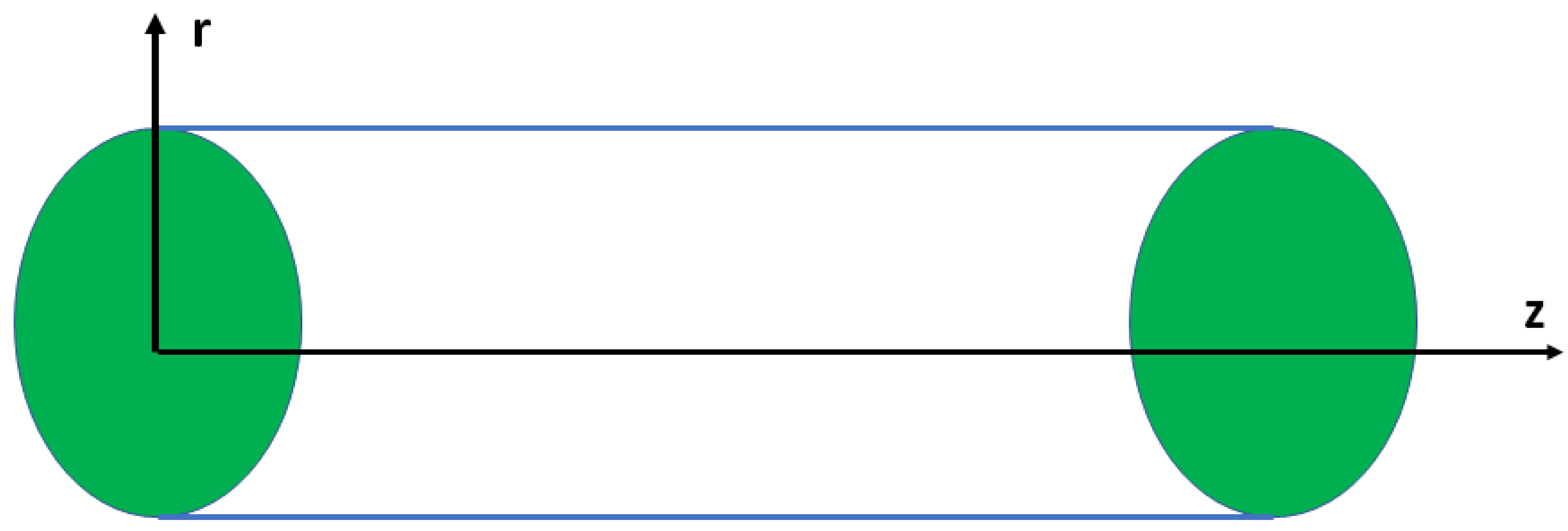
2.1. Domain Definition

Introduce cylindrical coordinate system $(r,\theta ,z)$ and consider laminar flow of incompressible viscoelastic fluid along z axis of infinitely long pipe of radius R with circular cross-section. The domain of interest is shown in Figure 1. The governing equations are momentum and continuity that read as:

$$\rho \frac{d\mathit{u}}{dt}=-\nabla p+\mathrm{div}\sigma$$

(1)

$$\mathrm{div}\mathit{u}=0,$$

(2)

where $\rho ,\mathit{u},p,\sigma$ are fluid mass density, flow velocity, pressure, and stress, respectively and $\frac{d}{dt}$ stands for total derivative. Provided $\mathit{u}={\mathit{u}}_z(r,t){\mathit{e}}_{\mathit{z}}$, where ${\mathit{e}}_{\mathit{z}}$ is a unit vector in z-direction and all but ${\sigma }_{rz}$ stress tensor components are set to 0, the momentum equation reduces to:

$$\rho \frac{\partial u_z}{\partial t}=-\frac{\partial p}{\partial z}+\frac{1}{r}\frac{\partial \left(r{\sigma }_{rz}\right)}{\partial r},$$

(3)

where $u_z$ stands for z-component of flow velocity and all other quantities are defined above. Additionally, we apply nonslip boundary condition at the wall.

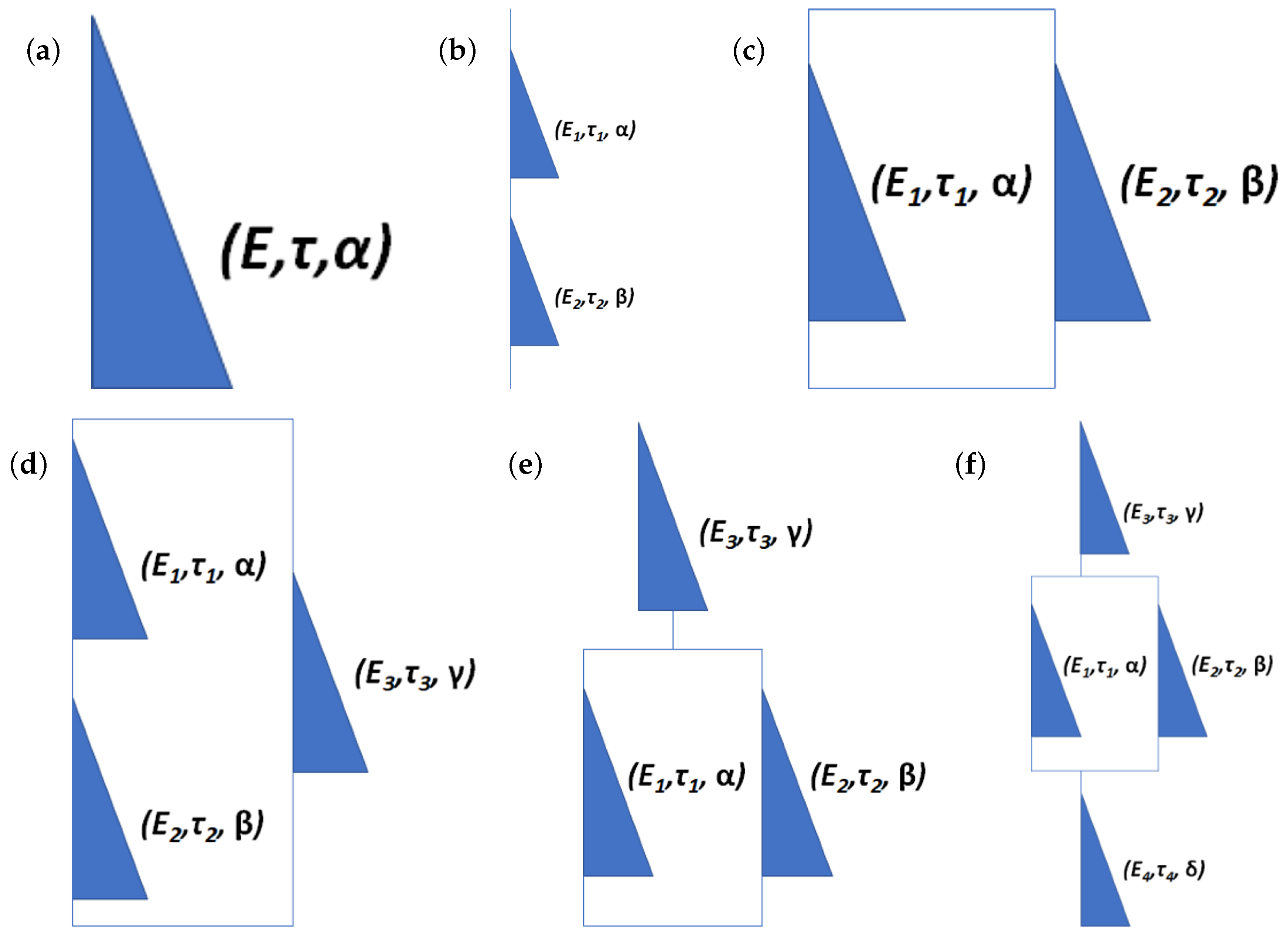
2.2. Fractional Element

The idea of introducing basic element accounting for both viscous and elastic properties of the material belongs to Blair [28]. Here we follow a conventional approach of constructing more complex mechanical models based on this element. For such an element, the stress-strain relation (constitutive equation) reads as:

$$\sigma \left(t\right)=E{\tau }^a{}_{\alpha }D_t^{\alpha }\epsilon \left(t\right),0\le \alpha \le 1,$$

(4)

where $\sigma \left(t\right),\epsilon \left(t\right),E,\tau ,\alpha$ stand for stress, strain, Young’s modulus, relaxation time and fractional order, respectively. The limiting cases of $\alpha =0$ and $\alpha =1$ represent spring and dashpot, respectively. The schematic of the element is given in Figure 2a. Here we use a conventional notation of Riemann–Liouville fractional derivative of a smooth function, $f\left(t\right)$, given by:

$${}_a{D}_t^{\alpha }f\left(t\right)=\frac{1}{\Gamma (k-\alpha )}\frac{d^k}{d{t}^k}{\int }_a^t{(t-t_0)}^{k-\alpha -1}f\left(t_0\right)d{t}_0,$$

(5)

where k is the integer, $\alpha$ is the fractional order, and $\Gamma (·)$ stands for Gamma-function defined as:

$$\Gamma \left(x\right)={\int }_0^{\infty }{\mathrm{e}}^{-t_0}{t}_0^{x-1}d{t}_0$$

(6)

In the following subsections we will provide constitutive equations for two-, three-, and four-component fractional viscoelastic models.

2.3. Fractional Maxwell Model

We start our consideration from the simplest yet commonly used two-component fractional model with basic elements connected in series (fractional Maxwell model, Figure 2b). The constitutive equation for this model reads as [39]:

$$\sigma \left(t\right)+{\tau }^{\alpha -\beta }{}_{a}D_t^{\alpha -\beta }\sigma \left(t\right)=E{\tau }^{\alpha }{}_{a}D_t^{\alpha }\epsilon \left(t\right),0\le \alpha \le 1,0\le \beta \le 1,\alpha \ge \beta ,$$

(7)

where $\alpha$ and $\beta$ stand for the fractional orders, $\tau ,E$ are defined as:

$$\tau ={\left(\frac{E_1{\tau }_1^{\alpha }}{E_2{\tau }_2^{\beta }}\right)}^{\frac{1}{\alpha -\beta }},E=E_1{\left(\frac{{\tau }_1}{\tau }\right)}^{\alpha },E=E_2{\left(\frac{{\tau }_2}{\tau }\right)}^{\beta },$$

(8)

and $E_1,{\tau }_1,E_2,{\tau }_2$ are the Young’s moduli, relaxation times for elements “1” and “2”, respectively. Constitutive equation of fractional Maxwell model (7) can be reduced to classical one, if $\alpha =1$ and $\beta =0$. Moreover, if we set $\alpha =1$ and $\beta =1$, Newtonian fluid can be obtained. The ranges set for fractional orders $\alpha$ and $\beta$ have both mathematical and physical meaning. Non-negative values of fractional orders and their difference reflect the fact that the dynamics of processes considered are described by fractional derivatives not fractional integrals. The upper limit of fractional orders range is set to get the corresponding classical viscoelastic model as a limiting case of a fractional one. For $\tau$ as it was defined above, $\alpha =\beta$ represents a special case. Indeed, it corresponds to relaxation time blowing up. Physically it means that a fluid becomes a critical gel. This special case is, however, beyond the scope of the current study. It is worth mentioning that relaxation time blows up only provided that the base of $\tau$ is greater than unity. If, however, that is not the case, i.e., $\tau$ base is less than unity, $\tau$ itself remains bound.

2.4. Fractional Kelvin–Voigt Model

Now let us connect two basic fractional elements in parallel. The dynamics of corresponding model (Kelvin–Voigt fractional model) are described as follows [39]:

$$\sigma \left(t\right)=E{\tau }^{\alpha }{}_{a}D_t^{\alpha }\epsilon \left(t\right)+E{\tau }^{\beta }{}_{a}D_t^{\alpha }\epsilon \left(t\right),E=E_2{\left(\frac{{\tau }_2}{\tau }\right)}^{\beta },$$

(9)

where all the notations are similar to those for fractional Maxwell model. The schematic of the model is given in Figure 2c. If $\alpha =1$ and $\beta =0$, we appear at classical Kelvin–Voigt model.

2.5. Fractional Zener Model

Let us now consider 3-element model referred to as fractional Zener model (Figure 2d). The corresponding constitutive equation reads as [39]:

$$\begin{array}{cc}\hfill \sigma \left(t\right)+{\tau }^{\alpha -\beta }{}_{a}D_t^{\alpha -\beta }\sigma \left(t\right)=& E{\tau }^{\alpha }{}_{a}D_t^{\alpha }\epsilon \left(t\right)+E_0{\tau }^{\gamma }{}_{a}D_t^{\gamma }\epsilon \left(t\right)+E_0{\tau }^{\gamma +\alpha -\beta }{}_{a}D_t^{\gamma +\alpha -\beta }\epsilon \left(t\right),\hfill \\ & 0\le \alpha \le 1,0\le \beta \le 1,0\le \gamma \le 1,\alpha -\beta \ge 0,\gamma +\alpha -\beta \ge 0,\end{array}$$

(10)

where $\gamma$ stands for the fractional order of element “3” and $E_0$ is given by:

$$E_0=E_3{\left(\frac{{\tau }_3}{\tau }\right)}^{\gamma },$$

(11)

with $E_3,{\tau }_3$ being Young’s modulus and relaxation time for element “3” and all other notations being the same as above. Assuming $\alpha =1$, $\beta =0$, and $\gamma =0$, classical Zener model can be restored.

2.6. Fractional Poynting–Thomson Model

For fractional Poynting–Thomson model (Figure 2e) the constitutive equation is [39]:

$$\begin{array}{cc}\hfill \sigma \left(t\right)+\frac{E}{E_0}{\tau }^{\alpha -\gamma }{}_{a}D_t^{\alpha -\gamma }\sigma \left(t\right)& +\frac{E}{E_0}{\tau }^{\beta -\gamma }{}_{a}D_t^{\beta -\gamma }\sigma \left(t\right)=E{\tau }^{\alpha }{}_{a}D_t^{\alpha }\epsilon \left(t\right)+E{\tau }^{\beta }{}_{a}D_t^{\alpha }\epsilon \left(t\right),\hfill \\ & 0\le \alpha \le 1,0\le \beta \le 1,0\le \gamma \le 1,\alpha -\gamma \ge 0,\beta -\gamma \ge 0,\end{array}$$

(12)

with all the notations similar to above, but different limitations applied to fractional orders $\alpha ,\beta$ and $\gamma$. Provided $\alpha =1$, $\beta =0$, and $\gamma =0$, we get classical Poynting–Thomson model.

2.7. Fractional Burgers Model

Finally, for the most complex, 4-element model considered in this study (fractional Burgers model, Figure 2f) the constitutive equation reads as [5]:

$$\begin{array}{c}\sigma \left(t\right)+\frac{E}{E_0}{\tau }_a^{\alpha -\gamma }{D}_t^{\alpha -\gamma }\sigma \left(t\right)+\frac{E}{E_0}{\tau }^{\alpha -\delta }{}_{a}D_t^{\alpha -\delta }\sigma \left(t\right)+\frac{E}{E_0}{\tau }_a^{\beta -\gamma }{D}_t^{\beta -\gamma }\sigma \left(t\right)+\frac{E}{E_0}{\tau }_a^{\beta -\delta }{D}_t^{\beta -\delta }\sigma \left(t\right)=\\ =E{\tau }^{\alpha }{}_{a}D_t^{\alpha }\epsilon \left(t\right)+E{\tau }_a^{\beta }{D}_t^{\beta }\epsilon \left(t\right),\\ 0\le \alpha \le 1,1\le \beta \le 2,0\le \gamma \le 1,0\le \delta \le 1,\alpha -\gamma \ge 0,\beta -\gamma \ge 0,\alpha -\delta \ge 0,\beta -\delta \ge 0\end{array}$$

(13)

where $\delta$ stands for the fractional order of element “4”, (11) is still valid and additionally:

$$E_0=E_4{\left(\frac{{\tau }_4}{\tau }\right)}^{\delta },$$

(14)

with $E_4,{\tau }_4$ being Young’s modulus and relaxation time for element “4” and all other notations being the same as above. If we set $\alpha =1$, $\beta =2$, $\gamma =0$, and $\delta =0$, classical Burgers model can be restored. Here $\beta -\gamma \ge 0$ and $\beta -\delta \ge 0$ are satisfied automatically, given the range for $\beta$, $\gamma$, and $\delta$.

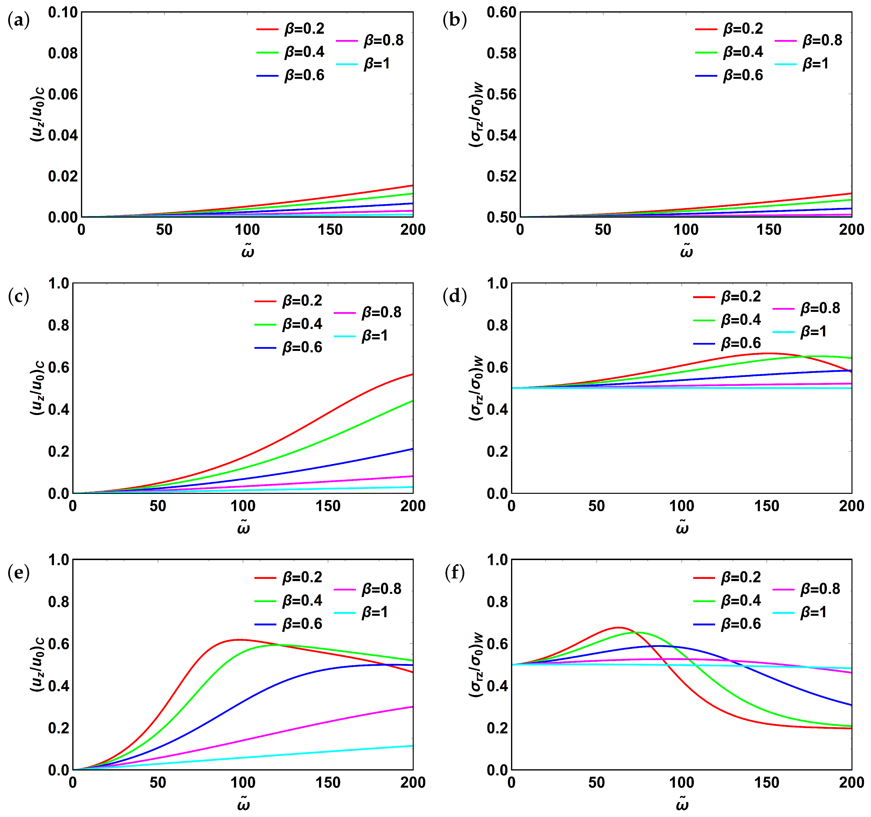
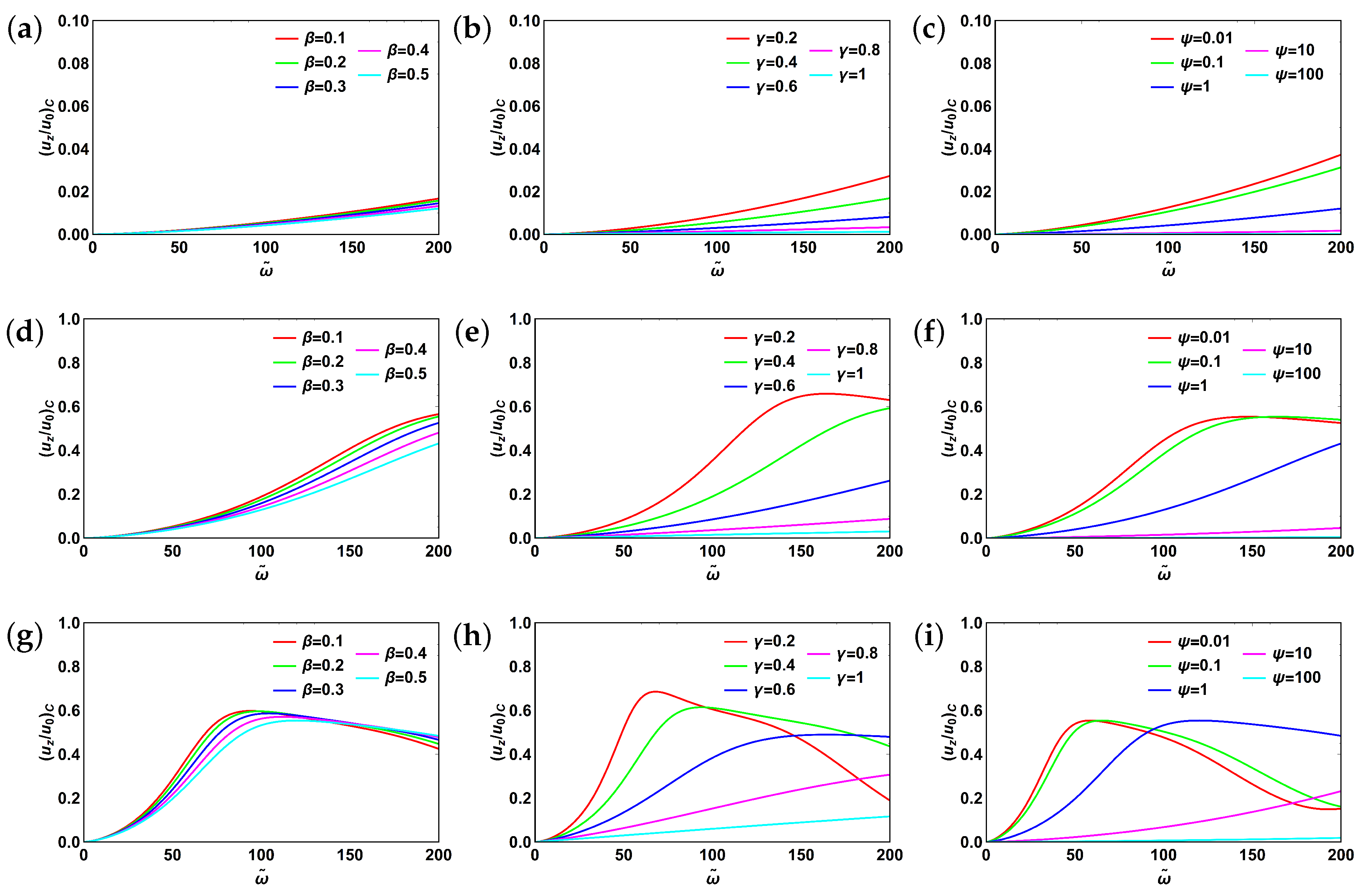
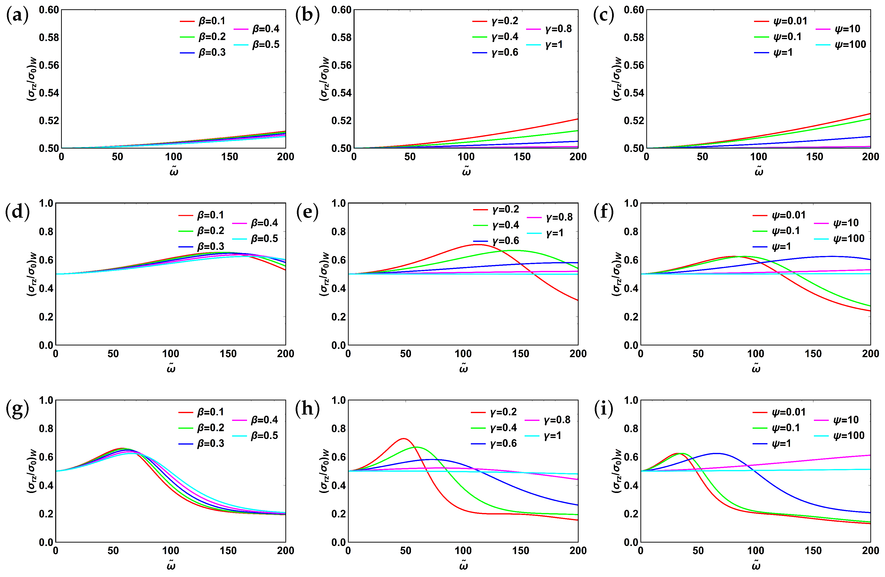
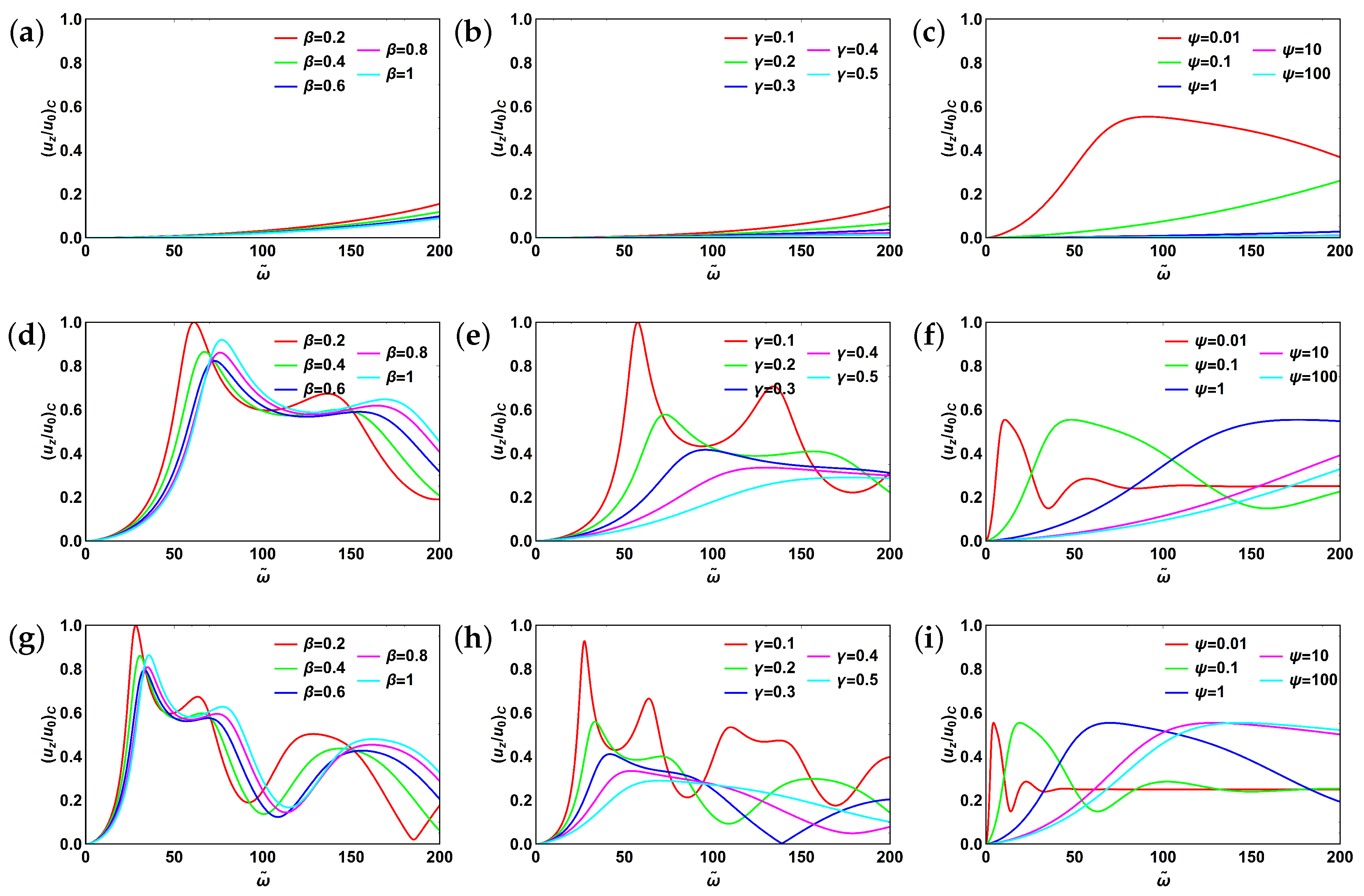
3. Results and Discussion

3.1. General Solution

Here we follow the approach proposed earlier by Yin [61] for Maxwell model and then generalize it for all other models. Consider a specific type of pressure gradient given as follows:

$$\frac{\partial p}{\partial z}=P_0{\mathrm{e}}^{i\omega t}$$

(15)

Introduce Fourier and inverse Fourier transforms of flow velocity and pressure:

$$U_z(r,\omega )={\int }_{-\infty }^{+\infty }{u}_z(r,t){\mathrm{e}}^{-i\omega t}dt,u_z(r,t)=\frac{1}{2\pi }{\int }_{-\infty }^{+\infty }{U}_z(r,\omega ){\mathrm{e}}^{i\omega t}d\omega$$

(16)

$$P(r,\omega )={\int }_{-\infty }^{+\infty }p(r,t){\mathrm{e}}^{-i\omega t}dt,p(r,t)=\frac{1}{2\pi }{\int }_{-\infty }^{+\infty }P(r,\omega ){\mathrm{e}}^{i\omega t}d\omega$$

(17)

Recall Fourier transform rule for fractional derivative:

$$\mathcal{F}{\{}_a{D}_t^{\alpha }{u}_z\}={\left(i\omega \right)}^{\alpha }{U}_z(r,\omega ),\mathcal{F}\left\{{}_{a}D_t^{\alpha -\beta }\frac{\partial p}{\partial z}\right\}={\left(i\omega \right)}^{\alpha -\beta }\frac{\partial P(r,\omega )}{\partial z},$$

(18)

where appropriate integration limits are implied. In particular, lower terminal value is set to: $a=-\infty$. Then the general algorithm to find flow velocity is the following: (1) express stress and its derivative from the constitutive eq-n; (2) plug stress and its derivative in momentum eq-n; (3) eliminate stress and its derivative and get modified momentum eq-n; (4) perform Fourier transform of modified momentum eq-n; (5) solve corresponding ODE for Fourier transform of velocity ($U_z(r,\omega )$); (6) change variables with $\xi$ for simplicity; (7) perform inverse Fourier transform of $U_z(r,\omega )$ to get $u_z(r,t)$. Regardless of the model considered, z-component of the velocity reads as:

$$u_z(r,t)=\frac{i}{\rho \omega }\frac{\partial p(z,t)}{\partial z}\left[1-\frac{J_0\left(\xi r\right)}{J_0\left(\xi R\right)}\right],$$

(19)

where $J_n(·)$ is the Bessel function of the first kind of order n. The only difference that defines behavior of the system is hidden in $\xi$. At the same time, the form of the solution reproduces a well-known classical result (see, for example Reference [73]). Thus it represents a natural extension of integer-order models using apparatus of FC. As long as velocity profile was defined, we could also get expression for the stress. The direct integration of (3) accounting for (15) results in:

$${\sigma }_{rz}=\frac{\partial p}{\partial z}\frac{J_1\left(\xi r\right)}{\xi J_0\left(\xi R\right)},$$

(20)

where again the individual properties of the model are hidden in parameter $\xi$. Physical meaning of $\xi$ is worth consideration. First, of all, $\left[\xi \right]=\left[1/\mathrm{m}\right]$, so that it can be considered as an “effective” wave number. Moreover, as shown below, $\xi$ is related to complex compliance. Introducing ${\sigma }_0=\frac{\partial p}{\partial z}R$, nondimensional stress $\tilde{\sigma }={\sigma }_{rz}/{\sigma }_0$ is given by:

$$\tilde{\sigma }=\frac{J_1\left(\xi r\right)}{\xi R{J}_0\left(\xi R\right)}$$

(21)

For practical purposes and analysis simplification, it is more convenient to introduce the following nondimensional quantities and relationships:

$$\tilde{r}=\frac{r}{\sqrt{\nu \tau }},\tilde{a}=\frac{R}{\sqrt{\nu \tau }},\tilde{\omega }=\omega \tau ,\varphi =\frac{\tilde{r}}{\tilde{a}},u_0=\frac{1}{4\rho \omega }\frac{\partial p}{\partial z},r^2{\xi }^2=\overline{\omega }{\tilde{r}}^2,$$

(22)

where $\nu$ is a kinematic viscosity and all other quantities were defined earlier. Then velocity and stress profiles are given by:

$$\tilde{u}=\left|\frac{u_z}{u_0}\right|=\left(1-\frac{J_0\left(\sqrt{\overline{\omega }}\tilde{a}\varphi \right)}{J_0\left(\sqrt{\overline{\omega }}\tilde{a}\right)}\right),\tilde{\sigma }=\left|\frac{{\sigma }_{rz}}{{\sigma }_0}\right|=\frac{J_1\left(\sqrt{\overline{\omega }}\tilde{a}\varphi \right)}{\sqrt{\overline{\omega }}\tilde{a}{J}_0\left(\sqrt{\overline{\omega }}\tilde{a}\right)}$$

(23)

As velocity profiles and shear stresses have been defined, we can now proceed with considering specific fractional viscoelastic models and outlining their specifics. Six parameters will be considered: fractional order ($\alpha ,\beta ,\gamma ,\delta$), nondimensional radius, $\tilde{a}$, and elastic ratio, $\psi$.

3.2. Fractional Maxwell Model

Let us start from the simplest two-parameter fractional Maxwell model. As outlined above, the key quantity that defines the behavior of a model is $\xi$. For this model $\xi$ is given by:

$${\xi }^2=\frac{\rho {\omega }^2}{E}\left[\frac{1}{{\left(i\omega \tau \right)}^{\alpha }}+\frac{1}{{\left(i\omega \tau \right)}^{\beta }}\right],$$

(24)

or alternatively in nondimensional form:

$$\overline{\omega }={\tilde{\omega }}^2\left[\frac{1}{{\left(i\tilde{\omega }\right)}^{\alpha }}+\frac{1}{{\left(i\tilde{\omega }\right)}^{\beta }}\right]$$

(25)

Centerline velocity profiles for fractional Maxwell model are shown in Figure 3. For all the plots $\alpha =0.5$. The value of $\tilde{a}$ ranges from $\tilde{a}=0.01$ (Figure 3a) to $\tilde{a}=0.1$ (Figure 3c). For this model an additional condition is imposed: $\alpha \ge \beta$, thus only a half of $\beta$ range is considered given the value of $\alpha$ set. As can be seen from this figure, the behavior of centerline velocity changes dramatically from monotonically increasing to resonant or oscillatory. Centerline velocity profile also changes with increasing fractional order ($\beta$). For lower values of $\tilde{a}$, an increase of $\beta$ results in decreasing of centerline velocity up to the constant value (as $\beta \to 0.5$). For higher values of $\tilde{a}$ (Figure 3b,c) the system exhibits aperiodic oscillations at low $\beta$ and demonstrates a switch from resonant behavior to monotonically increasing as $\beta$ increases. It is also worth mentioning that peak values decrease with increasing $\beta$. What is the reason for such a dramatic change of a velocity profile dynamics with varying $\tilde{a}$? In fact, ${\tilde{a}}^2$ turns out to be nothing else but a Reynolds number: ${\tilde{a}}^2=Re$, one of the key flow parameters.

Now let us have a look at the shear stress dynamics (at the wall) shown in Figure 4. Here again we fix $\alpha =0.5$ and vary $\beta$ ($\alpha \ge \beta$). Similar to velocity profile, shear stress increases monotonically with $\tilde{\omega }$ for lower values of $\tilde{a}$. The trend, however, changes to almost constant with increasing fractional order. As $\tilde{a}$ increases, the system exhibits more complex behaviors. In particular, there are aperiodic oscillations observed for lower values of fractional order that switch to resonant ones and monotonic decay as the fractional order starts to increase. Moreover, peak values shift to higher values of $\tilde{\omega }$ with increasing fractional order and the peaks themselves become more dispersive. At the same time, an increase of $\tilde{a}$ results in resonant peaks becoming sharper and shifting to lower values of $\tilde{\omega }$.

Finally, for relatively high values of $\tilde{\omega }$ and $\tilde{a}$, shear stress plots converge and become nearly independent from the fractional order $\beta$. To better understand physical meaning behind fractional orders $\alpha$ and $\beta$, we have examined its influence on centerline velocity and shear stress dynamics in a wider range of $\tilde{\omega }$ ($0\le \tilde{\omega }\le 1000$) with the fixed value of $\tilde{a}$ ($\tilde{a}=0.1$) as shown in Figure 5. We have first fixed $\alpha =0.5$ and varied $\beta$: $0.1\le \beta \le 0.5$. For both centerline velocity (Figure 5a) and shear stress (Figure 5b) low values of $\beta$ resulted in oscillatory profiles that in turn reflects the fact that the fractional order $\beta$ describes elastic properties of the fluid considered. In contrast, if we fix $\beta =0.5$ and vary $\alpha$: $0.6\le \alpha \le 1$, the oscillations are damped much quicker for both centerline velocity and shear stress (Figure 5c,d). Finally, let us set $\alpha =1$ and vary $\beta$: $0.25\le \beta \le 1$. Corresponding plots for centerline velocity and shear stress are shown in Figure 5e,f, respectively. When $\alpha =1$ and $\beta =1$, Newtonian fluid is obtained with centerline velocity monotonically reaching constant value and shear stress monotonically decaying.

3.3. Fractional Kelvin–Voigt Model

Next, we consider another commonly used two-parameter fractional model referred to as Kelvin–Voigt. We start from parameter $\xi$, responsible for system behavior. It reads as:

$${\xi }^2=\frac{\rho {\omega }^2}{E}\left[\frac{1}{{\left(i\omega \tau \right)}^{\alpha }+{\left(i\omega \tau \right)}^{\beta }}\right],$$

(26)

or alternatively in nondimensional form:

$$\overline{\omega }=\frac{{\tilde{\omega }}^2}{\left[{\left(i\tilde{\omega }\right)}^{\alpha }+{\left(i\tilde{\omega }\right)}^{\beta }\right]}$$

(27)

In contrast to fractional Maxwell model, no additional relations between $\alpha$ and $\beta$ are implied here. Thus, we have more freedom to set the values of these fractional orders within the entire range.

Centerline velocity profiles and shear stresses for fractional Kelvin–Voigt model are given in Figure 6. Here again we fix $\alpha =0.5$ and vary $\beta$. Different from fractional Maxwell model, centerline velocity profiles (Figure 6a,c,e) do not exhibit aperiodic oscillations with varying both fractional order and $\tilde{a}$. Centerline velocity amplitudes increase with increasing $\tilde{a}$ and decrease with increasing fractional order $\beta$. Shear stresses’ dynamics for the same model are presented in Figure 6b,d,f. Here again all three types of behavior encountered for fractional Maxwell model are present. More specifically, as $\tilde{a}$ increases, shear stresses experience three different types of behavior: from monotonically increasing through resonant to oscillatory. Relative stress amplitudes decrease with increasing fractional order $\beta$.

3.4. Fractional Zener Model

Now examine the behavior of three-element fractional Zener model. The key model variable, $\xi$, in this case becomes:

$${\xi }^2=\frac{\rho {\omega }^2}{E}\left[\frac{1}{(E_0/E){\left(i\omega \tau \right)}^{\gamma }+\frac{{\left(i\omega \tau \right)}^{\alpha +\beta }}{{\left(i\omega \tau \right)}^{\alpha }+{\left(i\omega \tau \right)}^{\beta }}}\right],$$

(28)

or alternatively in nondimensional form:

$$\overline{\omega }=\frac{{\tilde{\omega }}^2}{\psi {\left(i\tilde{\omega }\right)}^{\gamma }+\frac{{\left(i\tilde{\omega }\right)}^{\alpha +\beta }}{{\left(i\tilde{\omega }\right)}^{\alpha }+{\left(i\tilde{\omega }\right)}^{\beta }}},$$

(29)

where $\psi =\frac{E_0}{E}$ is an elastic parameter. By definition elastic parameter $\psi$ can be rewritten as:

$$\psi =\frac{E_3{\tau }_3^{\gamma }}{E_1{\tau }_1^{\alpha }}{\tau }^{\gamma -\alpha }$$

(30)

For classical Zener model ($\alpha =1$, $\beta =0$, and $\gamma =0$), $\psi$ reduces to: $\psi =E_3/E_2$, i.e., The ratio of Young’s moduli, thus justifying the notion introduced above. Similar to fractional Maxwell model, we impose additional conditions for fractional orders $\alpha$, $\beta$, and $\gamma$. From two inequalities: $\alpha -\beta \ge 0$ and $\gamma +\alpha -\beta \ge 0$, we end up with the first one. The second one is satisfied automatically, provided the first one is and $\gamma$ being non-negative.

We first examine the dynamics of centerline velocity. Different from two-element models, where we considered the influence of three parameters ($\alpha$, $\beta$, and $\tilde{a}$) on the system behavior, here we need to account for five parameters ($\tilde{a}$, $\alpha$, $\beta$, $\gamma$ and $\psi$). Let us fix $\alpha =0.5$ (as previously), $\gamma =0.5$ and $\psi =1$. Since $\alpha -\beta \ge 0$, we only consider $0\le \beta \le 0.5$. Corresponding centerline velocity profiles are given in Figure 7a,d,g. Centerline velocity changes its behavior from monotonically increasing to resonant with increasing $\tilde{a}$. Moreover, relative velocity amplitudes increase with increasing $\tilde{a}$. In addition to it, an interesting phenomenon is observed in Figure 7g. Relative velocity amplitudes tend to decrease with increasing fractional-order $\beta$ up to a certain value ($\tilde{\omega }\sim$ 150). At this point, centerline velocities for all fractional orders become close, and then the trend inverses, namely velocity amplitudes start to increase with increasing fractional-order $\beta$.

Next, let us fix $\alpha =\beta =0.5$, $\psi =1$ varying $\gamma$ and $\tilde{a}$. The corresponding plots for centerline velocity are shown in Figure 7b,e,h. Here we can observe switching from monotonically increasing to resonant behavior of the system with $\tilde{a}$ increasing and relative velocity amplitude decrease with increasing fractional order $\gamma$. Moreover, for larger values of $\tilde{a}$ centerline velocity behavior changes from resonant to almost linearly increasing with increasing fractional order $\gamma$.

Finally, we fixed $\alpha =\beta =\gamma =0.5$ and varied $\tilde{a}$ and $\psi$ as shown in Figure 7c,f,i. As can be seen, the system behavior changes from monotonically increasing to resonant with increasing $\tilde{a}$. Moreover, resonant curves become less dispersive, with increasing $\tilde{a}$ and more dispersive with increasing $\psi$. Relative amplitudes of centerline velocity also decrease with increasing $\psi$.

The dynamics of shear stresses are given in Figure 8. The first column in Figure 8 (Figure 8a,d,g) corresponds to $\alpha =\gamma =0.5$, $\psi =1$ and varying $\tilde{a}$ and $\beta$. In Figure 8g there exist two values of $\tilde{\omega }$ where shear stresses become very close for different values of fractional order $\beta$. Upon reaching the one corresponding to lower value of $\tilde{\omega }$, the trend reverses with relative stress amplitude decreasing for increasing fractional order, $\beta$. For large values of $\tilde{\omega }$, shear stress becomes almost independent of the fractional order, $\beta$. For the second column of Figure 8 (Figure 8b,e,h), we set $\alpha =\beta =0.5$, $\psi =1$ and varied $\tilde{a}$ along with $\gamma$. The new phenomenon observed can be seen in Figure 8e,h. That is, the resonant behavior changes to monotonically increasing and finally to constant with increasing fractional order $\gamma$. The similar trend is observed in case of varying $\psi$ as shown in Figure 8c,f,i ($\alpha =\beta =\gamma =0.5$).

3.5. Fractional Poynting–Thomson Model

The next model to be considered is fractional Poynting–Thomson one. Here $\xi$ reads as:

$${\xi }^2=\frac{\rho {\omega }^2}{E}\left[\frac{1}{(E_0/E){\left(i\omega \tau \right)}^{\gamma }}+\frac{1}{\left({\left(i\omega \tau \right)}^{\alpha }+{\left(i\omega \tau \right)}^{\beta }\right)}\right],$$

(31)

or alternatively in nondimensional form:

$$\overline{\omega }={\tilde{\omega }}^2\left(\frac{1}{\psi {\left(i\tilde{\omega }\right)}^{\gamma }}+\frac{1}{{\left(i\tilde{\omega }\right)}^{\alpha }+{\left(i\tilde{\omega }\right)}^{\beta }}\right)$$

(32)

Here we impose two additional conditions for fractional orders $\alpha$, $\beta$, and $\gamma$: $\alpha -\gamma \ge 0$ and $\beta -\gamma \ge 0$. As previously, we first examine the behavior of centerline velocity (Figure 9). Fixing $\alpha =\gamma =0.2$, $\psi =1$, we vary $\tilde{a}$ and $\beta$. The trends are somewhat repeatable compared to fractional Maxwell model (Figure 3a,d,g) and demonstrate elastic behavior for the entire range of $\beta$. Next, we fixed $\alpha =\beta =0.2$, $\psi =1$ and varied $\tilde{a}$ along with fractional order $\gamma$. The corresponding plots are presented in Figure 9b,e,h. Here aperiodic oscillations for lower values of fractional order $\gamma$, oscillatory and monotonically increasing velocity profiles with increasing $\gamma$ are observed. Finally, we set $\alpha =\beta =\gamma =0.5$ and varied $\tilde{a}$ and $\psi$ (Figure 9c,f,i). Here, resonant behavior is observed even for lower values of $\tilde{a}$ (Figure 9c). Moreover, for $\psi <1$ aperiodic oscillations of velocity are observed followed by it becoming independent from $\tilde{\omega }$. The trend, however, changes to resonant for $\psi >1$. Overall, the velocity oscillations are damped slower with $\psi$ increasing.

The shear stress dynamics at the wall are shown in Figure 10. As previously, we first fixed $\alpha =\gamma =0.2$, $\psi =1$ and varied $\tilde{a}$ and $\beta$ (Figure 10a,d,g). After major peak, shear stress drops dramatically with oscillations being damped for the entire range of $\beta$, except for Figure 10a, where it increases monotonically. The value of the major peak itself oscillates with increasing $\beta$. Next, as shown in Figure 10b,e,h, system parameters were set at $\alpha =\beta =0.2$, $\psi =1$ with varying $\tilde{a}$ and $\gamma$. Monotonically increasing trend for lower values of $\tilde{a}$ changes to aperiodic oscillations and resonant for higher ones. Moreover, the value of the major peak decreases monotonically with increasing fractional order $\gamma$. Finally, we set $\alpha =\beta =\gamma =0.5$ and varied $\tilde{a}$ and $\psi$. The corresponding plots are shown in Figure 10c,f,i. As can be seen from it, resonant behavior is present for all values of $\tilde{a}$. However, it switches to monotonically increasing with increasing $\psi$. Moreover, the switch happens at higher values of $\psi$ as $\tilde{a}$ increases and is absent for $\tilde{a}=0.1$ (Figure 10i).

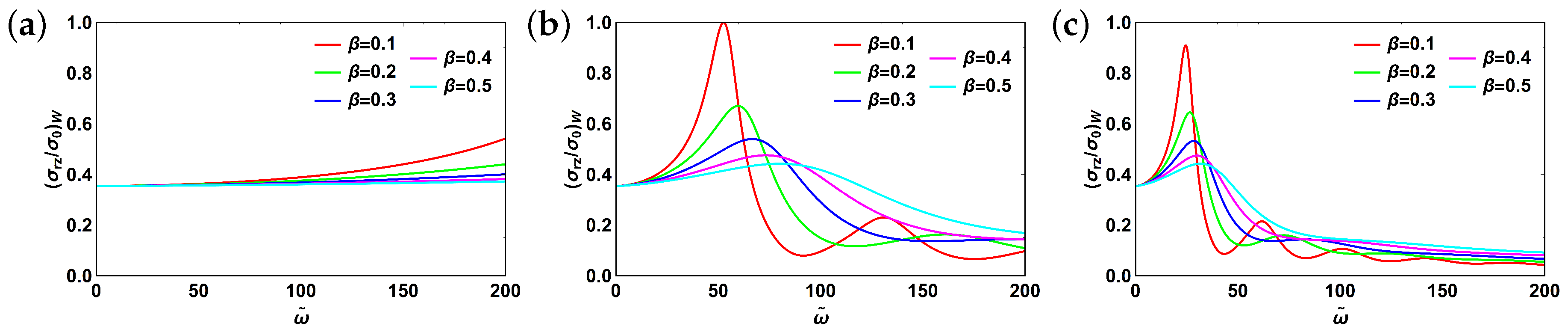
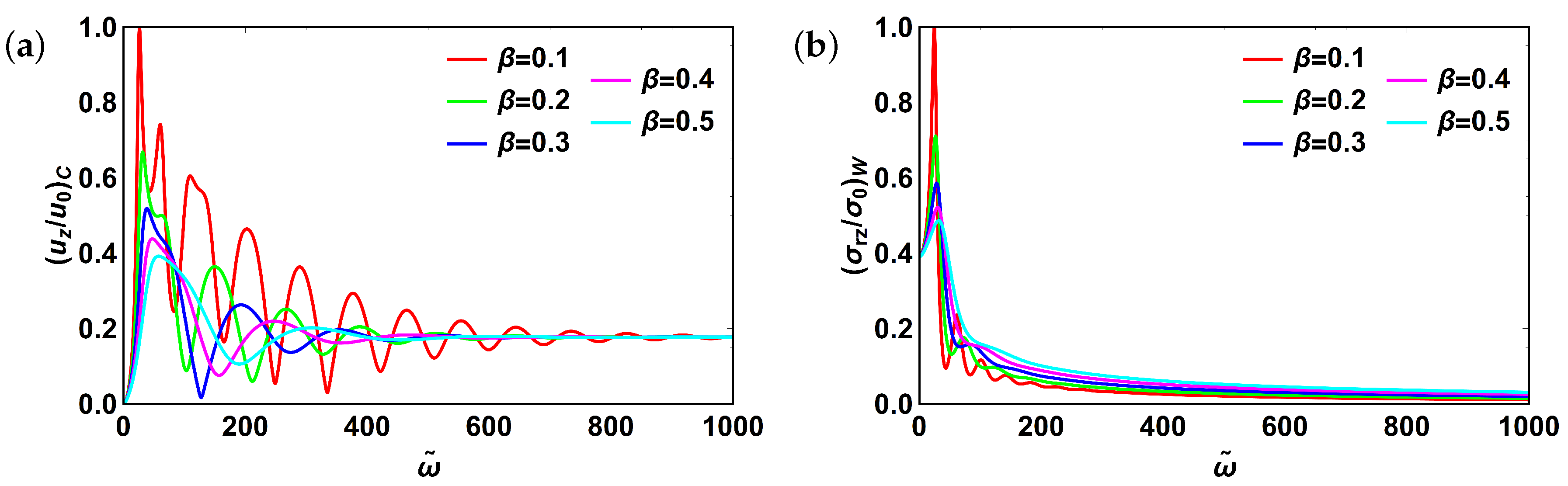
3.6. Fractional Burgers Model

Here we discuss the most complex fractional viscoelastic model, Burgers model. For this model $\xi$ is given by:

$${\xi }^2=\frac{\rho {\omega }^2}{E}\left[\frac{1}{(E_0/E)\left({\left(i\omega \tau \right)}^{\gamma }+{\left(i\omega \tau \right)}^{\delta }\right)}+\frac{1}{\left({\left(i\omega \tau \right)}^{\alpha }+{\left(i\omega \tau \right)}^{\beta }\right)}\right],$$

(33)

or alternatively in nondimensional form:

$$\overline{\omega }={\tilde{\omega }}^2\left(\frac{1}{\psi [{\left(i\tilde{\omega }\right)}^{\gamma }+{\left(i\tilde{\omega }\right)}^{\delta }]}+\frac{1}{{\left(i\tilde{\omega }\right)}^{\alpha }+{\left(i\tilde{\omega }\right)}^{\beta }}\right)$$

(34)

It is worth noting that for fractional Burgers model the range of fractional orders differs from all other models considered above. In particular, while the range for orders $\alpha$, $\gamma$, and $\delta$ is still from 0 to 1, $1\le \beta \le 2$. This change affects the dynamics of the centerline velocity profile dramatically. Centerline velocity profiles are shown in Figure 11. We first fixed $\alpha =\gamma =\delta =0.5$, $\psi =1$ and varied $\tilde{a}$ and $\beta$. The corresponding plots are shown in Figure 11a,d,g. The profile appears to be independent from the fractional order $\beta$. The situation changes when we set $\beta =1.5$ and vary $\delta$ (Figure 11b,e,h). Velocity profile is very sensitive to the changes in fractional order $\delta$ when it has relatively low values. Aperiodic oscillations with reducing peak values for increasing values of $\delta$ are observed. For varying $\psi$ (Figure 11 c,f,i), trends are overall similar to that for the fractional Poynting–Thomson model with the peaks for the fractional Burgers model being slightly sharper. This similarity can be attributed to the specific values of the fractional orders $\alpha$, $\gamma$ and $\delta$ set in Figure 11c,f,i ($\alpha =\gamma =\delta =0.5$). This specific setting has consequences for constitutive equations in both models. That is, the terms containing fractional derivatives of the orders $\alpha -\gamma$ and $\alpha -\delta$ become of the order zero.

Finally, let us have a look at the shear stresses shown in Figure 12. As can be seen from it, shear stress, too, is independent from the fractional order $\beta$ (Figure 12a,d,g). Stress dynamics change in Figure 12b,e,h. Quickly decaying aperiodic oscillations are observed. In particular, major peak values decrease monotonically with increasing value of fractional order $\delta$. Moreover, these peaks become sharper and shift to lower values of $\tilde{\omega }$ with increasing $\tilde{a}$. Next, we fixed $\alpha =\gamma =\delta =0.5$ and $\beta =1.5$. Here we observed resonant behavior for all values of $\tilde{a}$ and quickly damped oscillations for low values of $\psi$ (Figure 12c,f,i).

A closer look at expressions for $\xi$ corresponding to different models reveals their similarity. To illustrate this statement, let us introduce complex compliance, $J^{*}\left(\omega \right)$. For all the models considered, it has the following functional form: $[...]/E$, where an expression in square brackets is model-specific. Both $\xi$ and $\overline{\omega }$ can be expressed in terms of complex compliance:

$${\xi }^2=\rho {\omega }^2{J}^{*}\left(\omega \right),\overline{\omega }={\tilde{\omega }}^{2}E{J}^{*}\left(\omega \right),$$

(35)

as it was defined in [39]. Thus, generally speaking, $\xi$ is a complex quantity. Moreover, as we got complex compliance, other physical quantities including creep compliance, complex modulus, and relaxation modulus can be restored. For instance, $J^{*}\left(\omega \right)=1/G^{*}\left(\omega \right)$, where $G^{*}\left(\omega \right)$ stands for complex modulus. Then for fractional Maxwell model the loss modulus, $G^{″}\left(\omega \right)=\mathrm{Im}\left(G^{*}\left(\omega \right)\right)$, reads as [39]:

$$G^{″}\left(\omega \right)=E\frac{{\left(\omega \tau \right)}^{\alpha }sin(\pi \alpha /2)+{\left(\omega \tau \right)}^{2\alpha -\beta }sin(\pi \beta /2)}{1+{\left(\omega \tau \right)}^{2(\alpha -\beta )}+2{\left(\omega \tau \right)}^{\alpha -\beta }cos(\pi (\alpha -\beta )/2)}$$

(36)

Another insight can be obtained upon examination of Figure 2b–f and corresponding constitutive equations. The general observation is that more complex models can be obtained via consecutive combination of simpler ones with fractional elements. In particular, by adding fractional element to fractional Maxwell model in parallel, we arrive at fractional Zener model. Alternatively, starting from fractional Kelvin–Voigt model and adding fractional element in series, we get fractional Poynting–Thomson model. Adding one more fractional element in series, we end up with fractional Burgers model. The same “additive” behavior is observed for complex compliances.

It is worth emphasizing the generality of the approach developed. Provided the flow is axisymmetric, the pipe having a circular cross-section, and no-slip condition at the wall is satisfied, the solutions derived are suitable for various viscoelastic models commonly used for practical applications. For the same form of the solution of velocity and stress profiles, the prediction of flow dynamics for completely different fluids can be obtained via deriving a single model parameter, $\xi$. Moreover, the functional form of $\xi$ itself is also identical for all the models considered. What makes a given model specific is the expression for the complex compliance. This powerful approach simplifies significantly the implementation of other possible viscoelastic models within a given framework. The classical viscoelastic and Newtonian fluid models present the limiting cases of the theoretical approach proposed in this study. Velocity profiles’ dynamics for fractional Maxwell and Newtonian fluids in a circular pipe are shown in Supplementary Materials 1. These clearly demonstrate the complexity of behavior for fractional Maxwell model.

4. Conclusions

We have obtained exact analytical solutions for velocity profiles and shear stresses. Fractional Maxwell, Kelvin-Voigt, Zener, Poynting–Thomson, and Burgers models were considered. We demonstrated that the same form of the solution is applicable to all the models considered, thus generalizing prior studies. For both centerline velocity and shear profiles, three types of behavior (monotonically increasing, resonant, oscillating aperiodic) have been identified. In addition to it, switching between trends of relative velocity amplitudes have been predicted. Monotonically decreasing trends were found to be typical for relatively low values of normalized pipe radius with more complex behaviors taking place for higher values of the normalized radius. In addition to this, centerline velocity profiles featured almost constant plateaus. The proposed models cover the widest range of viscoelastic materials both in terms of the balance between viscous and elastic properties (via fractional-order) and the ratio of elastic properties for complex materials.

The approach we developed features an advantage that is worth mentioning. It allows the wide range of fractional viscoelastic models to be represented and solved in the same functional form. In fact, the entire system behavior can be described by a single function $\xi$ (or $\overline{\omega }$). It, in turn, is related to a complex compliance with the functional form identical for all five models considered in this study. Knowing complex compliance, complex and relaxation moduli and creep compliance are readily obtained. These quantities can be directly measured thus providing immediate practical applications for materials analysis. However, for some specific fields (e.g., polymers), experimental creep compliance data for short times has not been well-established so far. This problem was outlined in recent studies (see, for example, Reference [74]). It definitely deserves attention of the research community and will hopefully be addressed in future studies.

References

1. Leibniz, G. Letter from Hanover, Germany, to GFA L’Hopital, September 30; 1695. Math. Schriften 1849, 2, 301–302. [Google Scholar]
2. Ross, B. The development of fractional calculus 1695–1900. Hist. Math. 1977, 4, 75–89. [Google Scholar] [CrossRef] [Green Version]
3. Miller, K.S.; Ross, B. An Introduction to the Fractional Calculus and Fractional Differential Equations; Wiley: Hoboken, NJ, USA, 1993. [Google Scholar]
4. Podlubny, I. Fractional Differential Equations: An Introduction to Fractional Derivatives, Fractional Differential Equations, to Methods of their Solution and Some of their Applications; Elsevier: Amsterdam, The Netherlands, 1998. [Google Scholar]
5. Mainardi, F. Fractional Calculus: Theory and Applications; MDPI: Basel, Switzerland, 2018. [Google Scholar]
6. Hilfer, R. (Ed.) Applications of Fractional Calculus in Physics; World Scientific: Singapore, 2000; Volume 35. [Google Scholar]
7. Herrmann, R. Fractional Calculus: An Introduction for Physicists; World Scientific: Singapore, 2014. [Google Scholar]
8. Tarasov, V. Handbook of Fractional Calculus with Applications, Volume 4: Applications in Physics, Part A; De Gruyter: Berlin, Germany, 2019. [Google Scholar]
9. Tarasov, V. Handbook of Fractional Calculus with Applications, Volume 5: Applications in Physics, Part B; De Gruyter: Berlin, Germany, 2019. [Google Scholar]
10. Baleanu, D.; Lopes, A.M. Handbook of Fractional Calculus with Applications, Volume 7: Applications in Engineering, Life and Social Sciences, Part A; De Gruyter: Berlin, Germany, 2019. [Google Scholar]
11. Baleanu, D.; Lopes, A.M. Handbook of Fractional Calculus with Applications, Volume 8: Applications in Engineering, Life and Social Sciences, Part B; De Gruyter: Berlin, Germany, 2019. [Google Scholar]
12. Atanacković, T.M.; Janev, M.; Pilipović, S. On the thermodynamical restrictions in isothermal deformations of fractional Burgers model. Philos. Transact. R. Soc. A 2020, 378, 20190278. [Google Scholar] [CrossRef]
13. Chen, R.; Wei, X.; Liu, F.; Anh, V.V. Multi-term time fractional diffusion equations and novel parameter estimation techniques for chloride ions sub-diffusion in reinforced concrete. Philos. Transact. R. Soc. A 2020, 378, 20190538. [Google Scholar] [CrossRef] [PubMed]
14. Li, S.N.; Cao, B.Y. Fractional-order heat conduction models from generalized Boltzmann transport equation. Philos. Transact. R. Soc. A 2020, 378, 20190280. [Google Scholar] [CrossRef] [PubMed]
15. Bologna, E.; Di Paola, M.; Dayal, K.; Deseri, L.; Zingales, M. Fractional-order nonlinear hereditariness of tendons and ligaments of the human knee. Philos. Transact. R. Soc. A 2020, 378, 20190294. [Google Scholar] [CrossRef] [PubMed]
16. Chugunov, V.; Fomin, S. Effect of adsorption, radioactive decay and fractal structure of matrix on solute transport in fracture. Philos. Transact. R. Soc. A 2020, 378, 20190283. [Google Scholar] [CrossRef] [PubMed]
17. Failla, G.; Zingales, M. Advanced materials modelling via fractional calculus: Challenges and perspectives. Philos. Transact. R. Soc. A 2020, 378, 20200050. [Google Scholar] [CrossRef]
18. Fang, C.; Shen, X.; He, K.; Yin, C.; Li, S.; Chen, X.; Sun, H. Application of fractional calculus methods to viscoelastic behaviours of solid propellants. Philos. Transact. R. Soc. A 2020, 378, 20190291. [Google Scholar] [CrossRef]
19. Ionescu, C.M.; Birs, I.R.; Copot, D.; Muresan, C.; Caponetto, R. Mathematical modelling with experimental validation of viscoelastic properties in non-Newtonian fluids. Philos. Transact. R. Soc. A 2020, 378, 20190284. [Google Scholar] [CrossRef]
20. Li, J.; Ostoja-Starzewski, M. Thermo-poromechanics of fractal media. Philos. Transact. R. Soc. A 2020, 378, 20190288. [Google Scholar] [CrossRef] [PubMed]
21. Tenreiro Machado, J.; Lopes, A.M.; de Camposinhos, R. Fractional-order modelling of epoxy resin. Philos. Transact. R. Soc. A 2020, 378, 20190292. [Google Scholar] [CrossRef] [PubMed]
22. Di Paola, M.; Alotta, G.; Burlon, A.; Failla, G. A novel approach to nonlinear variable-order fractional viscoelasticity. Philos. Transact. R. Soc. A 2020, 378, 20190296. [Google Scholar] [CrossRef]
23. Patnaik, S.; Hollkamp, J.P.; Semperlotti, F. Applications of variable-order fractional operators: A review. Proc. R. Soc. A 2020, 476, 20190498. [Google Scholar] [CrossRef] [Green Version]
24. Patnaik, S.; Semperlotti, F. Variable-order particle dynamics: Formulation and application to the simulation of edge dislocations. Philos. Transact. R. Soc. A 2020, 378, 20190290. [Google Scholar] [CrossRef]
25. Povstenko, Y.; Kyrylych, T. Fractional thermoelasticity problem for an infinite solid with a penny-shaped crack under prescribed heat flux across its surfaces. Philos. Transact. R. Soc. A 2020, 378, 20190289. [Google Scholar] [CrossRef] [PubMed]
26. Zhang, X.; Ostoja-Starzewski, M. Impact force and moment problems on random mass density fields with fractal and Hurst effects. Philos. Transact. R. Soc. A 2020, 378, 20190591. [Google Scholar] [CrossRef] [PubMed]
27. Zorica, D.; Oparnica, L. Energy dissipation for hereditary and energy conservation for non-local fractional wave equations. Philos. Transact. R. Soc. A 2020, 378, 20190295. [Google Scholar] [CrossRef] [PubMed]
28. Blair, G.S. The role of psychophysics in rheology. J. Coll. Sci. 1947, 2, 21–32. [Google Scholar] [CrossRef]
29. Bagley, R.L.; Torvik, P. A theoretical basis for the application of fractional calculus to viscoelasticity. J. Rheol. 1983, 27, 201–210. [Google Scholar] [CrossRef]
30. Gloeckle, W.G.; Nonnenmacher, T.F. Fractional integral operators and Fox functions in the theory of viscoelasticity. Macromolecules 1991, 24, 6426–6434. [Google Scholar] [CrossRef]
31. Metzler, R.; Schick, W.; Kilian, H.G.; Nonnenmacher, T.F. Relaxation in filled polymers: A fractional calculus approach. J. Chem. Phys. 1995, 103, 7180–7186. [Google Scholar] [CrossRef]
32. Friedrich, C.; Braun, H. Generalized Cole-Cole behavior and its rheological relevance. Rheol. Acta 1992, 31, 309–322. [Google Scholar] [CrossRef]
33. Friedrich, C. Relaxation and retardation functions of the Maxwell model with fractional derivatives. Rheol. Acta 1991, 30, 151–158. [Google Scholar] [CrossRef]
34. Nonnenmacher, T.; Glöckle, W. A fractional model for mechanical stress relaxation. Philos. Mag. Lett. 1991, 64, 89–93. [Google Scholar] [CrossRef]
35. Schiessel, H.; Blumen, A. Mesoscopic pictures of the sol-gel transition: Ladder models and fractal networks. Macromolecules 1995, 28, 4013–4019. [Google Scholar] [CrossRef]
36. Schiessel, H.; Blumen, A. Hierarchical analogues to fractional relaxation equations. J. Phys. A Math. Gen. 1993, 26, 5057. [Google Scholar] [CrossRef]
37. Schiessel, H.; Blumen, A.; Alemany, P. Dynamics in disordered systems. In Transitions in Oligomer and Polymer Systems; Springer: Berlin, Germany, 1994; pp. 16–21. [Google Scholar]
38. Heymans, N.; Bauwens, J.C. Fractal rheological models and fractional differential equations for viscoelastic behavior. Rheol. Acta 1994, 33, 210–219. [Google Scholar] [CrossRef]
39. Schiessel, H.; Metzler, R.; Blumen, A.; Nonnenmacher, T. Generalized viscoelastic models: Their fractional equations with solutions. J. Phys. A Math. Gen. 1995, 28, 6567. [Google Scholar] [CrossRef]
40. Friedrich, C.; Schiessel, H.; Blumen, A. Constitutive behavior modeling and fractional derivatives. In Rheology Series; Elsevier: Amsterdam, The Netherlands, 1999; Volume 8, pp. 429–466. [Google Scholar]
41. Hernández-Jiménez, A.; Hernández-Santiago, J.; Macias-Garcıa, A.; Sánchez-González, J. Relaxation modulus in PMMA and PTFE fitting by fractional Maxwell model. Polym. Test. 2002, 21, 325–331. [Google Scholar] [CrossRef]
42. Makris, N.; Constantinou, M. Spring-viscous damper systems for combined seismic and vibration isolation. Earthq. Eng. Struct. Dyn. 1992, 21, 649–664. [Google Scholar] [CrossRef]
43. Zhang, Y.; Xu, S.; Zhang, Q.; Zhou, Y. Experimental and theoretical research on the stress-relaxation behaviors of PTFE coated fabrics under different temperatures. Adv. Mater. Sci. Eng. 2015, 2015, 319473. [Google Scholar] [CrossRef] [PubMed] [Green Version]
44. Khajehsaeid, H. Application of fractional time derivatives in modeling the finite deformation viscoelastic behavior of carbon-black filled NR and SBR. Polym. Test. 2018, 68, 110–115. [Google Scholar] [CrossRef]
45. Khajehsaeid, H. A Comparison Between Fractional-Order and Integer-Order Differential Finite Deformation Viscoelastic Models: Effects of Filler Content and Loading Rate on Material Parameters. Int. J. Appl. Mech. 2018, 10, 1850099. [Google Scholar] [CrossRef]
46. Yin, B.; Hu, X.; Song, K. Evaluation of classic and fractional models as constitutive relations for carbon black–filled rubber. J. Elastom. Plast. 2018, 50, 463–477. [Google Scholar] [CrossRef]
47. Xu, H.; Jiang, X. Creep constitutive models for viscoelastic materials based on fractional derivatives. Comp. Math. Appl. 2017, 73, 1377–1384. [Google Scholar] [CrossRef]
48. Stankiewicz, A. Fractional Maxwell model of viscoelastic biological materials. In BIO Web of Conferences; EDP Sciences: Les Ulis, France, 2018; Volume 10, p. 02032. [Google Scholar]
49. Farno, E.; Baudez, J.C.; Eshtiaghi, N. Comparison between classical Kelvin-Voigt and fractional derivative Kelvin-Voigt models in prediction of linear viscoelastic behaviour of waste activated sludge. Sci. Total Environ. 2018, 613, 1031–1036. [Google Scholar] [CrossRef]
50. Grace, S. XCIV. Oscillatory motion of a viscous liquid in a long straight tube. Lond. Edinb. Dublin Philos. Mag. J. Sci. 1928, 5, 933–939. [Google Scholar] [CrossRef]
51. Sexl, T. Uber den von EG Richardson entdeckten “Annulareffekt”. Z. Phys. 1930, 61, 349–362. [Google Scholar] [CrossRef]
52. Womersley, J.R. Method for the calculation of velocity, rate of flow and viscous drag in arteries when the pressure gradient is known. J. Physiol. 1955, 127, 553. [Google Scholar] [CrossRef]
53. Womersley, J.R. XXIV, Oscillatory motion of a viscous liquid in a thin-walled elastic tube—I: The linear approximation for long waves. Lond. Edinb. Dublin Philos. Mag. J. Sci. 1955, 46, 199–221. [Google Scholar] [CrossRef]
54. Uchida, S. The pulsating viscous flow superposed on the steady laminar motion of incompressible fluid in a circular pipe. Z. Angew. Math. Phys. ZAMP 1956, 7, 403–422. [Google Scholar] [CrossRef]
55. Taylor, M. An approach to an analysis of the arterial pulse wave II. Fluid oscillations in an elastic pipe. Phys. Med. Biol. 1957, 1, 321. [Google Scholar] [CrossRef] [PubMed]
56. Sergeev, S. Fluid oscillations in pipes at moderate Reynolds numbers. Fluid Dyn. 1966, 1, 121–122. [Google Scholar] [CrossRef]
57. Ramaprian, B.; Tu, S.W. An experimental study of oscillatory pipe flow at transitional Reynolds numbers. J. Fluid Mech. 1980, 100, 513–544. [Google Scholar] [CrossRef]
58. Harris, J.; Maheshwari, R. Oscillatory pipe flow: A comparison between predicted and observed displacement profiles. Rheol. Acta 1975, 14, 162–168. [Google Scholar] [CrossRef]
59. Hino, M.; Sawamoto, M.; Takasu, S. Experiments on transition to turbulence in an oscillatory pipe flow. J. Fluid Mech. 1976, 75, 193–207. [Google Scholar] [CrossRef]
60. Wood, W. Transient viscoelastic helical flows in pipes of circular and annular cross-section. J. Non Newton. Fluid Mech. 2001, 100, 115–126. [Google Scholar] [CrossRef]
61. Yin, Y.; Zhu, K.Q. Oscillating flow of a viscoelastic fluid in a pipe with the fractional Maxwell model. Appl. Math. Comp. 2006, 173, 231–242. [Google Scholar] [CrossRef]
62. Yang, D.; Zhu, K.Q. Start-up flow of a viscoelastic fluid in a pipe with a fractional Maxwell’s model. Comp. Math. Appl. 2010, 60, 2231–2238. [Google Scholar] [CrossRef] [Green Version]
63. Shah, S.H.A.M.; Qi, H. Starting solutions for a viscoelastic fluid with fractional Burgers’ model in an annular pipe. Nonlinear Anal. Real World Appl. 2010, 11, 547–554. [Google Scholar] [CrossRef]
64. Nazar, M.; Fetecau, C.; Awan, A. A note on the unsteady flow of a generalized second-grade fluid through a circular cylinder subject to a time dependent shear stress. Nonlinear Anal. Real World Appl. 2010, 11, 2207–2214. [Google Scholar] [CrossRef]
65. Qi, H.; Liu, J. Some duct flows of a fractional Maxwell fluid. Eur. Phys. J. Spec. Top. 2011, 193, 71–79. [Google Scholar] [CrossRef]
66. Khandelwal, K.; Mathur, V. Exact solutions for an unsteady flow of viscoelastic fluid in cylindrical domains using the fractional Maxwell model. Int. J. Appl. Comput. Math. 2015, 1, 143–156. [Google Scholar] [CrossRef] [Green Version]
67. Mathur, V.; Khandelwal, K. Exact Solutions for the Flow of Fractional Maxwell Fluid in Pipe-Like Domains. Adv. Appl. Math. Mech. 2016, 8, 784–794. [Google Scholar] [CrossRef]
68. Maqbool, K.; Mann, A.; Siddiqui, A.M.; Shaheen, S. Fractional generalized Burgers’ fluid flow due to metachronal waves of cilia in an inclined tube. Adv. Mech. Eng. 2017, 9, 1687814017715565. [Google Scholar] [CrossRef] [Green Version]
69. Tang, Y.; Zhen, Y.; Fang, B. Nonlinear vibration analysis of a fractional dynamic model for the viscoelastic pipe conveying fluid. Appl. Math. Model. 2018, 56, 123–136. [Google Scholar] [CrossRef]
70. Wang, Y.; Chen, Y. Dynamic Analysis of the Viscoelastic Pipeline Conveying Fluid with an Improved Variable Fractional Order Model Based on Shifted Legendre Polynomials. Fractal Fract. 2019, 3, 52. [Google Scholar] [CrossRef] [Green Version]
71. Javadi, M.; Noorian, M.; Irani, S. Stability analysis of pipes conveying fluid with fractional viscoelastic model. Meccanica 2019, 54, 399–410. [Google Scholar] [CrossRef]
72. Sun, H.; Zhang, Y.; Baleanu, D.; Chen, W.; Chen, Y. A new collection of real world applications of fractional calculus in science and engineering. Commun. Nonlinear Sci. Num. Simulat. 2018, 64, 213–231. [Google Scholar] [CrossRef]
73. Crandall, I.B. Theory of Vibrating Systems and Sound; D. Van Nostrand Company: New York, NY, USA, 1926. [Google Scholar]
74. Urbanowicz, K.; Duan, H.F.; Bergant, A.; Urbanowicz, K.; Bergant, H.F.D.A. Transient Liquid Flow in Plastic Pipes. STROJNISKI VESTNIK J. Mech. Eng. 2020, 66, 77–90. [Google Scholar] [CrossRef]
Figure 1. Domain definition for the circular pipe.
Applsci 10 09093 g001
Figure 2. Fractional models: (a) basic element; (b) Maxwell; (c) Kelvin–Voigt; (d) Zener; (e) Poynting–Thomson; (f) Burgers.
Applsci 10 09093 g002
Figure 3. Centerline velocity profile for fractional Maxwell model: (a) a ˜ = 0.01 ; (b) a ˜ = 0.05 ; (c) a ˜ = 0.1 . For all plots α = 0.5 . Subscript “c” stands for “centerline”.
Applsci 10 09093 g003
Figure 4. Shear stress profile at the pipe wall for fractional Maxwell model: (a) a ˜ = 0.01 ; (b) a ˜ = 0.05 ; (c) a ˜ = 0.1 . For all plots α = 0.5 . Subscript “w” stands for “wall”.
Applsci 10 09093 g004
Figure 5. Fractional Maxwell model: (a) centerline velocity, α = 0.5 ; (b) shear stress, α = 0.5 ; (c) centerline velocity, β = 0.5 ; (d) shear stress, β = 0.5 ; (e) centerline velocity, α = 1 ; (f) shear stress, α = 1 . For all plots a ˜ = 0.1 . Subscripts “c” and “w” stand for “centerline” and “wall”, respectively.
Applsci 10 09093 g005aApplsci 10 09093 g005b
Figure 6. Fractional Kelvin–Voigt model: (a) centerline velocity, a ˜ = 0.01 ; (b) shear stress, a ˜ = 0.01 ; (c) centerline velocity, a ˜ = 0.05 ; (d) shear stress, a ˜ = 0.05 ; (e) centerline velocity, a ˜ = 0.1 ; (f) shear stress, a ˜ = 0.1 . For all plots α = 0.5 . Subscripts “c” and “w” stand for “centerline” and “wall”, respectively.
Applsci 10 09093 g006
Figure 7. Centerline velocity for fractional Zener model: (a) a ˜ = 0.01 , α = γ = 0.2 , ψ = 1 ; (b) a ˜ = 0.01 , α = β = 0.5 , ψ = 1 ; (c) a ˜ = 0.01 , α = β = γ = 0.5 ; (d) a ˜ = 0.05 , α = γ = 0.2 , ψ = 1 ; (e) a ˜ = 0.05 , α = β = 0.5 , ψ = 1 ; (f) a ˜ = 0.05 , α = β = γ = 0.5 ; (g) a ˜ = 0.1 , α = γ = 0.2 , ψ = 1 ; (h) a ˜ = 0.1 , α = β = 0.5 , ψ = 1 ; (i) a ˜ = 0.1 , α = β = γ = 0.5 . Subscript “c” stands for “centerline”.
Applsci 10 09093 g007
Figure 8. Shear stress at the pipe wall for fractional Zener model: (a) a ˜ = 0.01 , α = γ = 0.2 , ψ = 1 ; (b) a ˜ = 0.01 , α = β = 0.5 , ψ = 1 ; (c) a ˜ = 0.01 , α = β = γ = 0.5 ; (d) a ˜ = 0.05 , α = γ = 0.2 , ψ = 1 ; (e) a ˜ = 0.05 , α = β = 0.5 , ψ = 1 ; (f) a ˜ = 0.05 , α = β = γ = 0.5 ; (g) a ˜ = 0.1 , α = γ = 0.2 , ψ = 1 ; (h) a ˜ = 0.1 , α = β = 0.5 , ψ = 1 ; (i) a ˜ = 0.1 , α = β = γ = 0.5 . Subscript “w” stands for “wall”.
Applsci 10 09093 g008
Figure 9. Centerline velocity for fractional Poynting-Thomson model: (a) a ˜ = 0.01 , α = γ = 0.2 , ψ = 1 ; (b) a ˜ = 0.01 , α = β = 0.5 , ψ = 1 ; (c) a ˜ = 0.01 , α = β = γ = 0.5 ; (d) a ˜ = 0.05 , α = γ = 0.2 , ψ = 1 ; (e) a ˜ = 0.05 , α = β = 0.5 , ψ = 1 ; (f) a ˜ = 0.05 , α = β = γ = 0.5 ; (g) a ˜ = 0.1 , α = γ = 0.2 , ψ = 1 ; (h) a ˜ = 0.1 , α = β = 0.5 , ψ = 1 ; (i) a ˜ = 0.1 , α = β = γ = 0.5 . Subscript “c” stands for “centerline”.
Applsci 10 09093 g009
Figure 10. Shear stress at the pipe wall for fractional Poynting-Thomson model: (a) a ˜ = 0.01 , α = γ = 0.2 , ψ = 1 ; (b) a ˜ = 0.01 , α = β = 0.5 , ψ = 1 ; (c) a ˜ = 0.01 , α = β = γ = 0.5 ; (d) a ˜ = 0.05 , α = γ = 0.2 , ψ = 1 ; (e) a ˜ = 0.05 , α = β = 0.5 , ψ = 1 ; (f) a ˜ = 0.05 , α = β = γ = 0.5 ; (g) a ˜ = 0.1 , α = γ = 0.2 , ψ = 1 ; (h) a ˜ = 0.1 , α = β = 0.5 , ψ = 1 ; (i) a ˜ = 0.1 , α = β = γ = 0.5 . Subscript “w” stands for “wall”.
Applsci 10 09093 g010
Figure 11. Centerline velocity for fractional Burgers model: (a) a ˜ = 0.01 , α = γ = 0.5 , ψ = 1 ; (b) a ˜ = 0.01 , α = β = 0.5 , ψ = 1 ; (c) a ˜ = 0.01 , α = β = γ = 0.5 ; (d) a ˜ = 0.05 , α = γ = 0.5 , ψ = 1 ; (e) a ˜ = 0.05 , α = β = 0.5 , ψ = 1 ; (f) a ˜ = 0.05 , α = β = γ = 0.5 ; (g) a ˜ = 0.1 , α = γ = 0.5 , ψ = 1 ; (h) a ˜ = 0.1 , α = β = 0.5 , ψ = 1 ; (i) a ˜ = 0.1 , α = β = γ = 0.5 . Subscript “c” stands for “centerline”.
Applsci 10 09093 g011
Figure 12. Shear strees at the pipe wall for fractional Burgers model: (a) a ˜ = 0.01 , α = γ = 0.5 , ψ = 1 ; (b) a ˜ = 0.01 , α = β = 0.5 , ψ = 1 ; (c) a ˜ = 0.01 , α = β = γ = 0.5 ; (d) a ˜ = 0.05 , α = γ = 0.5 , ψ = 1 ; (e) a ˜ = 0.05 , α = β = 0.5 , ψ = 1 ; (f) a ˜ = 0.05 , α = β = γ = 0.5 ; (g) a ˜ = 0.1 , α = γ = 0.5 , ψ = 1 ; (h) a ˜ = 0.1 , α = β = 0.5 , ψ = 1 ; (i) a ˜ = 0.1 , α = β = γ = 0.5 . Subscript “w” stands for “wall”.
Applsci 10 09093 g012
Publisher’s Note: MDPI stays neutral with regard to jurisdictional claims in published maps and institutional affiliations.