Article

Development of Post Processing for Wave Propagation Problem: Response Filtering Method

1
School of Mechanical Engineering, Hanyang University, Seoul 04763, Korea
2
Korea and Hyundai Motor Company, Seoul 06797, Korea
3
Department of Mathematics, Dongguk University, Seoul 04620, Korea
*
Author to whom correspondence should be addressed.
Appl. Sci. 2020, 10(24), 9032; https://doi.org/10.3390/app10249032
Submission received: 17 November 2020 / Revised: 11 December 2020 / Accepted: 12 December 2020 / Published: 17 December 2020
(This article belongs to the Special Issue Noise Reduction and Vibration Isolation)

Abstract

:
This study develops a new response filtering approach for recovering dynamic mechanical stresses under impact loading. For structural safety, it is important to consider the propagation of transient mechanical stresses inside structures under impact loads. Commonly, mechanical stress waves can be obtained by solving Newton’s second law using explicit or implicit finite element procedures. Regardless of the numerical approach, large discrepancies called the Gibb’s phenomenon are observed between the numerical solution and the analytical solution. To reduce these discrepancies and enhance the accuracy of the numerical solution, this study develops a response filtering method (RFM). The RFM averages the transient responses within split time domains. By solving several benchmark problems and analyzing the stresses in the frequency domain, it was possible to verify that the RFM can provide an improved solution that converges toward the analytical solution. A mathematical theory is also presented to correlate the relationship between the filtering length and the frequency components of the filtered stress values.

1. Introduction

This study develops a new response filtering approach for recovering dynamic mechanical stress under impact loads. From a structural engineering point of view, a mechanical stress wave, due to structural impacts such as an impact force, explosion, or collision, that propagates through a structural medium is important. When this wave reaches weak parts of the structure, it can cause unexpected catastrophic failure or fracturing of structural components. Thus, it is important to compute and consider these stress waves in mechanical or civil engineering [1,2,3,4]. With the use of state-of-the-art computational theory and computer hardware, numerical solutions can be regarded as acceptably close to the analytical solution. However, from a theoretical perspective, some discrepancies and errors remain, and verification of the convergence to the true solution is still important. Some efforts have been undertaken to reduce the differences and the numerical errors between the numerical solutions and analytical solutions [3,5,6]. To this end, this study develops a new post-processing approach for transient stress waves named the response filtering method (RFM) with an average operator.
Numerical methods, e.g., the finite element (FE) method, finite volume method, or finite difference method, have been employed for the transient analysis of complex structures. The numerical solutions obtained using proper computational theory usually converge to the analytical solutions with a refined time step and refined mesh [3,5,6]. However, it has been observed that it is f ˜ = f s F L m ± f difficult for a numerical solution to describe an analytical solution that has significant discontinuity, even when proper meshes and time steps are adopted. In finite element (FE) numerical solutions, overshooting, undershooting, and oscillations occur around the discontinuity point known as the Gibbs phenomenon [1,7,8,9]. Various studies have been conducted aiming to reduce these types of discrepancies between the analytical and numerical solutions. Some relevant research can be found to improve the numerical accuracy by introducing the numerical damping [10]. For instance, the discontinuous Galerkin method and variational integrator have been proposed to accurately describe discontinuities in the numerical solutions [11,12,13,14,15]. Other approaches have been proposed to reduce the dispersive and dissipative errors in the numerical solution of partial difference equations [3,4,16,17]. Klaus and Bathe make a significant contribution to the finite element method for wave propagation problem. They present higher-order spatially discretized finite elements with an extra computational cost for the wave propagation problem [3,16] and also present new implicit and explicit integration methods with Noh [4,17]. Linear combinations of consistent and lumped mass matrices [18,19,20] and modified spatial integration rules for mass and stiffness matrices [21,22] have been considered to ensure high-fidelity solutions. Comprehensive and considerable benchmark problems for wave propagation can be found in the work of Idesman et al. [23]. However, in numerical solutions, errors due to Gibb’s phenomenon cannot be eliminated completely, and some improvements are required to the oscillation of the numerical solution [9]. A few post-processing methods have been developed to reduce these kinds of numerical errors [21,23,24].
The objective of this study is not to develop a new finite element or integration method but to develop a simple post-processing approach, i.e., the RFM, to reduce discrepancies between the numerical and analytical solutions. In this study, only one-dimensional problems are considered to calculate exact solutions (analytical solution) as references. The transient stress values in the discrete time domain are simply divided into several subset domains, and each subset domain is averaged. The subsets have a specific number of stress values, which, in this paper, is called the filtering length. The averaged stress values are set as the filtered stress values, and the original stress values are replaced with the filtered values in the corresponding time domain, as shown in Figure 1. The RFM not only efficiently solves the oscillation problem in the numerical solution by adjusting the filtering length, but it also creates discontinuous solutions that converge to the analytical solutions. Alternatively, it can be considered that the RFM can create new frequency components of the responses (especially higher frequency components). In this study, the relationship between the RFM and frequency components is mathematically verified, and a formulation is introduced to predict the generated frequency components using RFM.
This remainder of this paper is organized as follows. In Section 2, the concept, application, and limitations of finite element formulations for the mechanical wave problem and numerical integration scheme, i.e., Newmark’s scheme, are reviewed. In Section 3, to resolve the oscillation issue, i.e., Gibb’s phenomenon in the numerical solution, the RFM is presented. In Section 4, several numerical examples are presented to demonstrate that the present RFM can be utilized to improve the accuracy of numerical solutions. Finally, Section 5 provides conclusions and directions for future research.

2. Finite Element Analysis for the Transient Stress Response

2.1. Transient Finite Element Simulation

The transient response of a mechanical structure can be analyzed using the finite element procedure as follows [3,5,6]:
U ¨ i = M 1 [ F i C U ˙ i K U i ]
where the mass, damping, and stiffness matrices are denoted by M , C , and K , respectively, and the force vector at the ith time step is denoted by F i , and the displacement, velocity, and acceleration vectors at the ith time step are denoted by U i , U ˙ i , and U ¨ i , respectively. Many numerical schemes can be applied to solve the above Newton’s law. This study implements both explicit and implicit integration method to investigate performance of the present RFM. Central-difference method and Newmark’s method are adopted as representation of explicit and implicit integration methods.
Central-difference method approximates velocity and acceleration by
U ˙ i = 1 2 Δ t ( U i + 1 U i 1 )
U ¨ i = 1 Δ t 2 ( U i + 1 2 U i + U i 1 )
and U i + 1 and U i 1  can be obtained by Taylor series about time iΔt:
U i + 1 = U i + Δ t 1 ! U ˙ i + Δ t 2 2 ! U ¨ i + Δ t 3 3 ! U i +
U i 1 = U i Δ t 1 ! U ˙ i + Δ t 2 2 ! U ¨ i Δ t 3 3 ! U i +
Combining Equations (2)–(5) with the second-order accuracy provides the following equation:
U i + 1 = [ 1 Δ t 2 M + 1 2 Δ t C ] 1 { F i K U i + 1 Δ t 2 M ( 2 U i U i 1 ) + 1 2 Δ t C U i 1 }
In Newmark’s method [3,5,6], displacement vector of i + 1th time step can be obtained as follows:
U ˙ i + 1 = U ˙ i + ( Δ t ) [ ( 1 γ ) U ¨ i + γ U ¨ i + 1 ]
U i + 1 = U i + ( Δ t ) U ˙ i + ( Δ t ) 2 [ ( 1 2 β ) U ¨ i + β U ¨ i + 1 ]
where Δt is the time step, and the two parameters of Newmark’s scheme are β and γ [6]. With the above approximations of Newmark’s method, the following discretized equations in the time domain can be obtained:
K U i + 1 = F i + 1 ,
K = M Δ t 2 β + γ Δ t β C + K ,
F i + 1 = F i + 1 + [ M + Δ t γ C Δ t 2 β ] U i + [ M + Δ t γ C Δ t β C ] U ˙ i + [ ( 1 2 β 1 ) ( M + Δ t γ C ) Δ t ( 1 γ ) C ] U ¨ i .
In this study, the coefficients of Newmark’s method, β and γ , are set to 1 4 and 1 2 , respectively for unconditional stability.
The dynamic stress at the ith time step can be calculated from the displacements at the ith time step as follows:
σ i = [ σ x σ y τ x y ] i = D B U i .
D = E 1 ν 2 [ 1 ν 0 ν 1 0 0 0 1 ν 2 ]
2 D   plane   stress :   σ i = σ x 2 σ x σ y + σ y 2 + 3 τ x y .
The plane stress (von Mises stress), stress vector, displacement vector, constitutive matrix, and strain–displacement matrix at the ith time step are denoted by σ i , σ i , U i , D , and B , respectively. The Young’s modulus and Poisson’s ratio are denoted by E and ν , respectively.

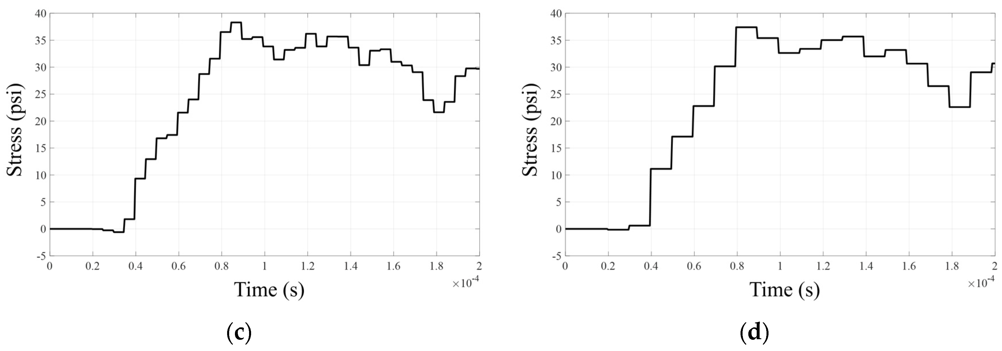
2.2. Wave Propagation Analysis and Gibb’s Phenomenon

Facilitated by the developments in hardware and software, finite element simulations of transient systems have been applied in many application areas [3]. Despite their successful applications, one of the remaining issues with transient finite element simulations is the Gibb’s phenomenon, with its associated overshooting and undershooting phenomena [5]. This issue becomes a serious problem in structural analyses. To illustrate this problem, let us consider the stress analysis in Figure 2 as an example [5]. The right side of a 20-in-long rectangular bar ( L T ) with a cross-sectional area (A) of 1 in2 is fixed, and a step load of 100 lb is applied in the x-direction on the left side of the bar at t = 0 . The Young’s modulus (E), density (ρ), and Poisson’s ratio ( ν ) of the bar are 30 × 10 6 psi, 7.4 × 10 4 lb-s2/in4, and zero (for a one-dimensional problem), respectively. In this study, the analysis domain is discretized using a 40 × 1 mesh of 4-node rectangular elements (Q4). The mesh size of this example is chosen by following the parameters and setting of the reference [5]. In addition, it is worth to note that the issues of the stability and the accuracy of the numerical integration schemes should be considered, and the time of this example is chosen to consider the stabilities of the numerical integration schemes. The time step (sampling time), Δ t , is set to 4.0 × 10 7   s smaller than the critical time (   Δ t c r = L c / v   ( = 2 . 483 × 10 6 ) , v : E / ρ , L c : characteristic length) for the stability of the central-difference method.
The transient finite element simulation determines the transient solution with application of a sudden load to the cross section. The stress of the cross section in the steady-state solution becomes 100 psi. Figure 3 shows the mechanical stress value calculated at x = 9.75 in (20th element). The solid and the dotted lines represent the analytical and numerical solutions, respectively. With mechanical properties we can calculate speed of wave propagation ( v = E / ρ = 2.012 × 10 5   in / s ) and time stress curve. Before the arrival time ( t 1 = 9.75 2.012 × 10 5 = 4.7214 × 10 5 s ), the stress values at x = 9.75 in are zero because the stress wave has not yet arrived. After the first arrival time and before the next arrival time ( t 2 = 9.75 + 2 × ( 20 9.75 ) 2.012 × 10 5 = 1.5158 × 10 4 s ), the analytical stress value becomes 100 psi. After 1.5148 × 10 4 s , the analytical stress value increases to 200 psi owing to the arrival of the reflected wave at the right side. The steady-state stress is 100 psi. The stress values obtained with the explicit and implicit method are plotted with exact solution in Figure 3. The overall tendency is similar to that of the analytical solution, but some spurious oscillations naturally occur. It is observed that larger oscillations occur at the areas of sharp transition ( t 1 = 4.7214 × 10 5 s and t 2 = 1.5158 × 10 4 s ). Comparing the analytical and numerical solutions, it seems that the numerical solution obtained using the transient finite element simulation contains additional frequencies. However, later we will demonstrate that the numerical solution actually cannot carry valuable information in the frequency domain compared with the analytical solution. From a mathematical perspective, this phenomenon is referred to as Gibb’s phenomenon and has been widely studied (see [4,5] and the references therein). In finite element theory, considering this phenomenon, the stability issue has been researched [4,5,9,14,16,20]. The present study revisits the Gibb’s phenomenon and presents a heuristic approach for improving the accuracy of finite element simulations.

3. Response Filtering Method for Improved Transient Stress

This section presents a new engineering approach, i.e., the RFM, to improve the transient stress calculated using the finite element approach. In static analysis, spatial-averaging approaches for the stress have been proposed, but to the best of our knowledge, an averaging scheme in the time domain has not been previously proposed.

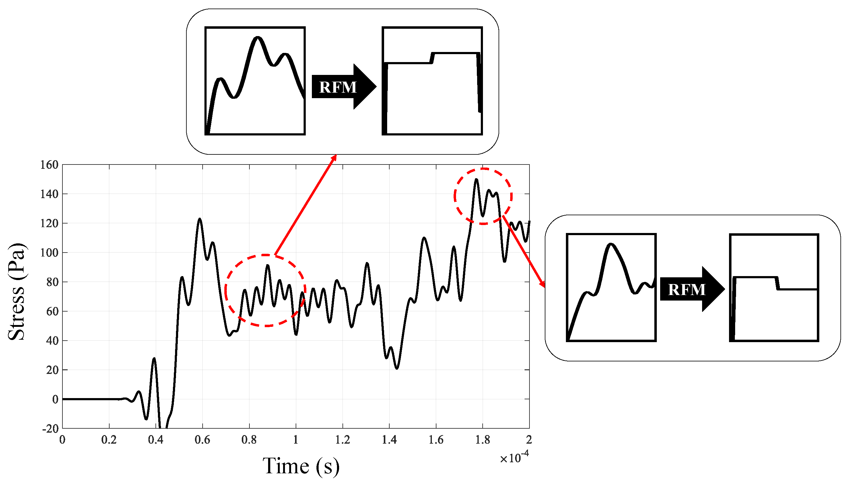
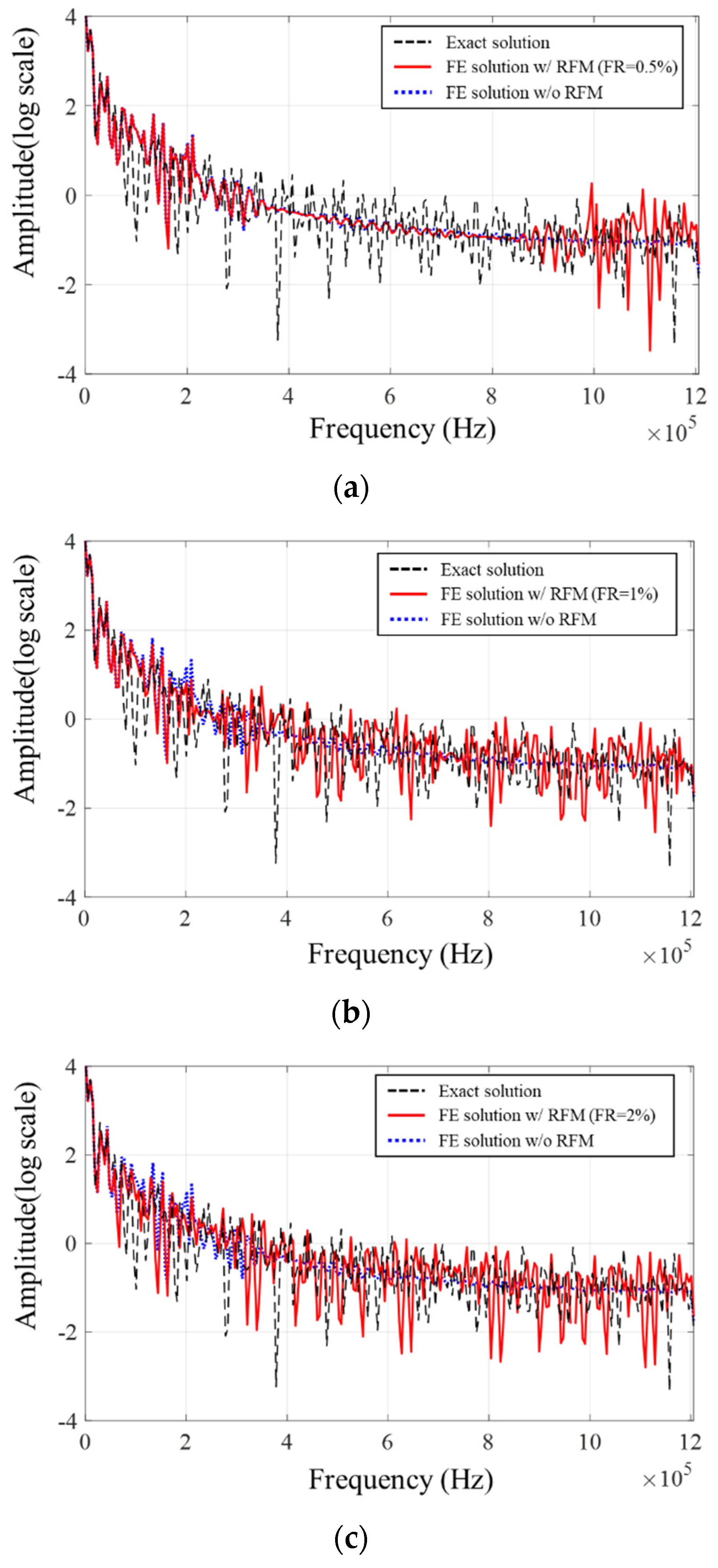
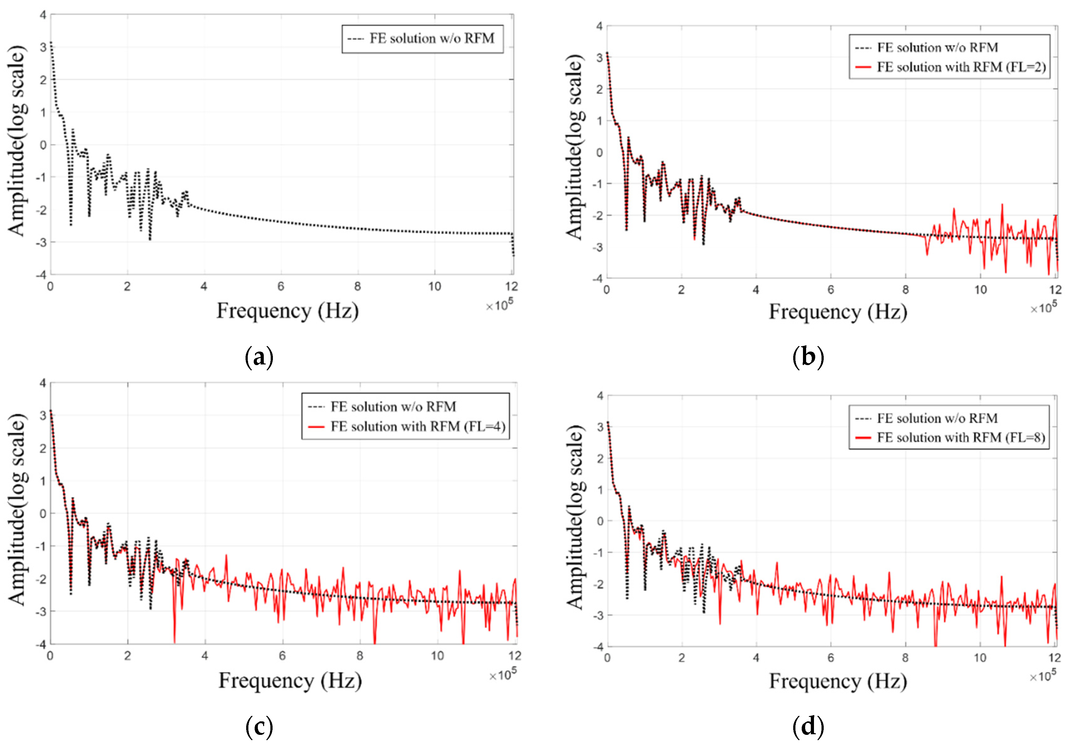
3.1. Response Filtering Method

As its name implies, the RFM filters the transient stress values in the time domain. A standard FE simulation is conducted to compute the transient stress values. As illustrated in the previous section, the Gibb’s phenomenon hinders our ability to obtain accurate solutions using this method. By investigating the responses and their characteristics, this study proposes the concept of averaging the erroneous transient stress values using the RFM. Through averaging, or filtering, it is expected that the oscillations can be cancelled out, and thus the accuracy of the computed transient stress values can be improved. This concept has been applied for the stress analysis of static structure systems and is implemented in various commercial software [25,26]. As it is a relatively simple concept, it is easy to implement in the post-processing stage of any FE package. The present study is confined to averaging (or filtering) in the time domain in order to illustrate the benefit of the proposed RFM.
Figure 1 illustrates a schematic diagram of the proposed RFM. First, the stress and displacement responses are computed in the time domain using a conventional numerical approach, i.e., Newmark’s method. The resulting transient solutions are approximations of the analytical solution, and oscillations inevitably occur due to the Gibb’s phenomenon. The displacement or stress response at each time step in the numerical approach can be described by (12), and without the loss of generality, the stress values are employed to illustrate the RFM.
σ = [ σ 1 , σ 2 , σ N 1 , σ N ]   ( N :   number   of   time   steps ) ,
where the (von Mises) stress of target element is denoted by σi, and the subscript i denotes the time step and set of stresses with respect to time step is σ. The transient stress values can be divided into NR regions and renumbered for convenience as follows:
σ = [ σ 1 , σ 2 , , σ F L the   1 st   region , σ F L + 1 , , σ 2 F L the   2 nd   region , , σ N F L + 1 , , σ N the   N R th   region ]   = [ σ 1 1 , σ 2 1 , , σ F L 1 the   1 st   region , σ 1 2 , , σ F L 2 the   2 nd   region , , σ 1 N R , , σ F L N R the   N R th   region ] .
The “region” defined in this research refers the time step region in which the solutions are averaged.
To avoid confusion in notation, the ith stress at the jth region is denoted by σ i j . The filter length, which is equal to the number of stress values in each region, is denoted by FL. The filtered stresses or responses are obtained by averaging with a weight factor as follows:
σ ˜   = [ σ ˜ 1 the   1 st region , , σ ˜ k the   k - th region , , σ ˜ N R the   N R - th region ] ,
σ ˜ k = [ σ ˜ 1 k , , σ ˜ j k , , σ ˜ F L k ] ,   ( σ ˜ 1 k = σ ˜ j k = σ ˜ F L k ) ,
σ ˜ j k = i = 1 F L w i k σ i k i = 1 F L w i k ,   k = 1 , 2 , , N R ,   j = 1 , 2 , , F L ( N = F L × N R ,   F R = F L N × 100 ) ,
where the set of original and filtered stresses (responses) at all time steps are denoted by σ and σ ˜ , respectively. The ith filtered stress and the weighting factor in the kth domain are denoted by σ j k and w j k , respectively. The filtering length, filtering ratio and number of the filtered regions are FL, FR, and NR, respectively. In the present study, the weight factors are set as equal to one. For example, the filtered stress in (17) with an FL value of two becomes the following:
σ ˜ = [ σ 1 + σ 2 2 , σ 1 + σ 2 2 σ ˜ 1 , σ 3 + σ 4 2 , σ 3 + σ 4 2 σ ˜ 2 , , σ N 1 + σ N 2 , σ N 1 + σ N 2 σ ˜ F L ]
This simple filtering approach, which is similar to the stress average in static FE analysis, is carried out in the time domain rather than in the spatial domain. To validate the performance of the proposed method, the benchmark problem in Section 2 can be revisited. The transient stresses of the benchmark problem in Figure 2 are filtered using the proposed RFM by varying the ratio of filter data, FR, in Figure 4. Moreover, the following norm-based absolute error for the stress (response) is employed to evaluate the performance of the present method for transient analysis:
ξ = | σ ¯ ( t ) σ ( t ) | d t   or   | σ ¯ ( t ) σ ˜ ( t ) | d t ,
where the exact (analytical), numerical, and filtered numerical solutions at time t are denoted by σ ¯ ( t ) and σ ˜ ( t ) , respectively. Figure 4 presents the tendency of the accuracy improvement of the RFM with varying filtering ratio, FR. Table 1 shows the performance of RFM with respect to filtering ratio (FR), the error valuer in Equation (21) is reduced by increasing FR by around 2% and also the number of oscillations is reduced as shown in Table 2. The table shows that the RFM could show similar performance regardless of integration methods. Approximately 2% of FR may show significant improvement in accuracy under different numerical conditions.
Because the proposed method yields an artificially generated piecewise constant solution, it has to be validated not only in time but also in space. Therefore, the benchmark problem in Figure 2 was conducted once more with different space condition. Both exact and numerical stress responses at x = 0.25 in (1st element) were calculated by the same procedure as the previous example. Lots of spurious oscillation was found around at second arrival time in the finite element method ( t = 20 + 19.75 2.012 × 10 5 ) in Figure 5. The detail performance of RFM with different filtering ratio, FR, is written in Table 2. Similar to the previous example, the FR (filtering ratio) value around 2% shows the improvement in time and space.

3.2. Analysis of the Accuracy Improvement with the Response Filtering Method

As shown in the previous section, the simple averaging procedure with the RFM results in significant improvements in the prediction compared to the analytical solution by generating piecewise constant solutions. For the sake of conducting an accuracy analysis of the proposed method, this subsection investigates the solutions using the Fourier transformation.
Without the loss of generality, a simple signal, y , with a 50 Hz frequency component was generated for 0.1 s with 100 samplings in Figure 6. In other words, y ( t ) = sin ( 2 π 50 t ) , and the sampling time, T s = 0.001   s . Figure 6a (left) and (right) shows the original signal and its Fourier transformation, respectively, with the peak at 50 Hz. Figure 6b–d shows the filtered signals with different filtering lengths and their transformations. These figures illustrate that the Fourier transformations of the filtered signals contain some additional frequency components. For example, with FL = 2, the filtered signal bears additional frequency components at 450 Hz. With FL = 4, frequencies around 200, 300, and 450 Hz are added, while with FL = 5, frequencies around 150, 250, 350, and 450 Hz are added. Furthermore, the signals in the time domain become rectangular in shape owing to these added frequency components. These analyses indicate that the filtering procedures used for the time signals actually generate additional frequencies. In addition, it is found that there is a rule for the emerging frequencies. For example, Figure 6a shows that the original signal has a single frequency component of 50 Hz, whereas the filtered signal (FL = 2) has an additional frequency component at 450 Hz in addition to the frequency component (50 Hz) of the original signal, as shown in Figure 6b.
Prior to determining the relationship between the filtering length and the added frequency components, it should be noted that the discrete Fourier transform (DFT) defines the following relationship between the analysis time and frequency:
T s = T 0 N ,   f 0 = f s N , f 0 = 1 T 0 , f s = 1 T s ,
where the number of time step, total analysis time and the sampling time ( Δ t ) are denoted by N , T 0 , and T s , respectively, and the frequency step ( Δ f ) and the sampling frequency are denoted by f 0 and f s , respectively. Using the above notations, this study formulates the following theory based on the DFT.
Theorem 1.
Consider the signal, y ˜ , filtered from original signal, y , which has only a single frequency component, f , with a filtering length FL. With sampling frequency, f s , the Fourier transformation of the filtered signal has the following frequency component:
f ˜ = f s F L m ± f   and   0 f ˜ f s 2 ,
where m and f ˜ denote an arbitrary integer and the frequency components generated by the frequency filtering method (i.e., the RFM), respectively. The frequency components generated by the filtering scheme in DFT can be mathematically found through the following proof.
Proof. 
The N-point DFT of discrete signal y k is obtained as follows:
Y n = 1 N k = 0 N 1 y k e j 2 π n N k .
Assuming y k = exp ( j 2 π f * N k ) (a signal with a single frequency component, f , where f * = f f 0 ), the above DFT can be summarized as follows:
Y n = 1 N k = 0 N 1 e j 2 π N ( n f * ) k = δ f ( n ) ,   δ f ( n ) = { 1   ( f * = n ) 0   ( f * n ) ,
where δ f ( n ) is the Kronecker delta function, and Equation (25) is used for the proof.
k = 0 N 1 a r k = { N a   ( r = 1 ) a ( 1 r N ) 1 r   ( r 1 ) ,
r = ( e j 2 π n N ) = 1 ,   ( n N = m ,   m   is   arbitrary   integer ) ,
( e j 2 π n N ) N = 1 .
The condition of Equation (27) can be satisfied only if m = 0 because N is always larger than n in Equation (25).
The DFT of the filtered signal, y ˜ , obtained from the RFM with FL can be formulated as follows:
Y ˜ n = 1 N l = 0 N / F L 1 y ˜ F L l [ e j 2 π n N F L l + e j 2 π n N ( F L l + 1 ) + + e j 2 π n N { F L l + F L 1 } ] = 1 N l = 0 N / F L 1 [ y F L l + y F L l + 1 + + y F L l + F L 1 ] F L [ e j 2 π n N F L l + e j 2 π n N ( F L l + 1 ) + + e j 2 π n N { F L l + F L 1 } ] = 1 N F L l = 0 N / F L 1 y F L l ( y 0 + + y F L 1 ) e j 2 π n N F L l ( e 0 + + e j 2 π n N { F L 1 } ) = 1 N F L ( i = 0 F L 1 e j 2 π f * N i i = 0 F L 1 e j 2 π n N i ) l = 0 N / F L 1 e j 2 π F L f * N l e j 2 π F L n N l = 1 N F L 1 e j 2 π F L N f * 1 e j 2 π N f * 1 e j 2 π F L N n 1 e j 2 π N n l = 0 N / F L 1 e j 2 π F L ( n f * ) N l = 1 N F L 1 e j 2 π F L N f * 1 e j 2 π N f * 1 e j 2 π F L N n 1 e j 2 π N n l = 0 N / F L 1 r l , ( r = e j 2 π F L ( n f * ) N )
Therefore, the Fourier transform of the filtered signal is given by Equations (25)–(28):
Y ˜ n = { 1 F L 2 1 e j 2 π F L N f * 1 e j 2 π N f * 1 e j 2 π F L N n 1 e j 2 π N n ( r = 1 )   0 ( r 1 )   .
The condition for r = e j 2 π F L ( n f * ) N = 1 can be simplified using Equation (27) as follows:
F L N ( n f * ) = m ,
n = N F L m + f * ,
where m represents an arbitrary integer. The integer domain can be transformed to the discrete frequency domain by multiplying the frequency step, f 0 , as follows:
f 0 n = f 0 N F L m + f 0 f * = f s F L m + f
The frequency components, f 0 n , generated by the RFM can be simply denoted by f ˜ , as in (23). With y k = sin ( k 2 π f * N ) = sin ( k 2 π f f s ) = e j k 2 π f f s e j k 2 π f f s 2 j ,   ( f * = f / f 0 , N = f s / f 0 ) , the DFT for this example can be expressed as follows:
Y n = { 1 2 j 1 F L 2 1 e j F L 2 π f f s 1 e j 2 π f f s 1 e j F L 2 π f ˜ f s 1 e j 2 π f s ( f ˜ = f s F L m + f ) 1 2 j 1 F L 2 1 e j F L 2 π f f s 1 e j 2 π f f s 1 e j F L 2 π f ˜ f s 1 e j 2 π f s ( f ˜ = f s F L m f ) 0   ( otherwise )
The range of (33) corresponds exactly to Theorem 1. Therefore, Theorem 1 is mathematically validated.
The locations of the newly created frequency components can be predicted using the sampling frequency (or sampling time), filtering length, and original frequency component with (23). For instance, a sampling frequency of 1000 Hz is used for the example in Figure 6. Therefore, the generated frequency components with respect to the filtering length can be calculated as summarized in Table 3. It is verified that Theorem 1 predicts the newly generated frequency components with the RFM in Figure 6 and Table 3.
Based on the above consideration, we revisit the previous example in Figure 2 with Fourier transformation. The time domain mechanical stress response at x = 9.75 in is transformed to frequency domain by DFT (the time domain response is calculated by Newmark’s method with Δ t = 4.0 × 10 7   s ). As shown in Figure 7, when the RFM is not applied, only the low-frequency components can be obtained. However, with the current RFM, several high-frequency components, which only can be obtained by piecewise constant components (red line) are generated. In addition, RFM, with a filtering ratio of 2% showing significant performance in previous time domain analyses, creates additional new frequency components that can cover all frequency ranges.

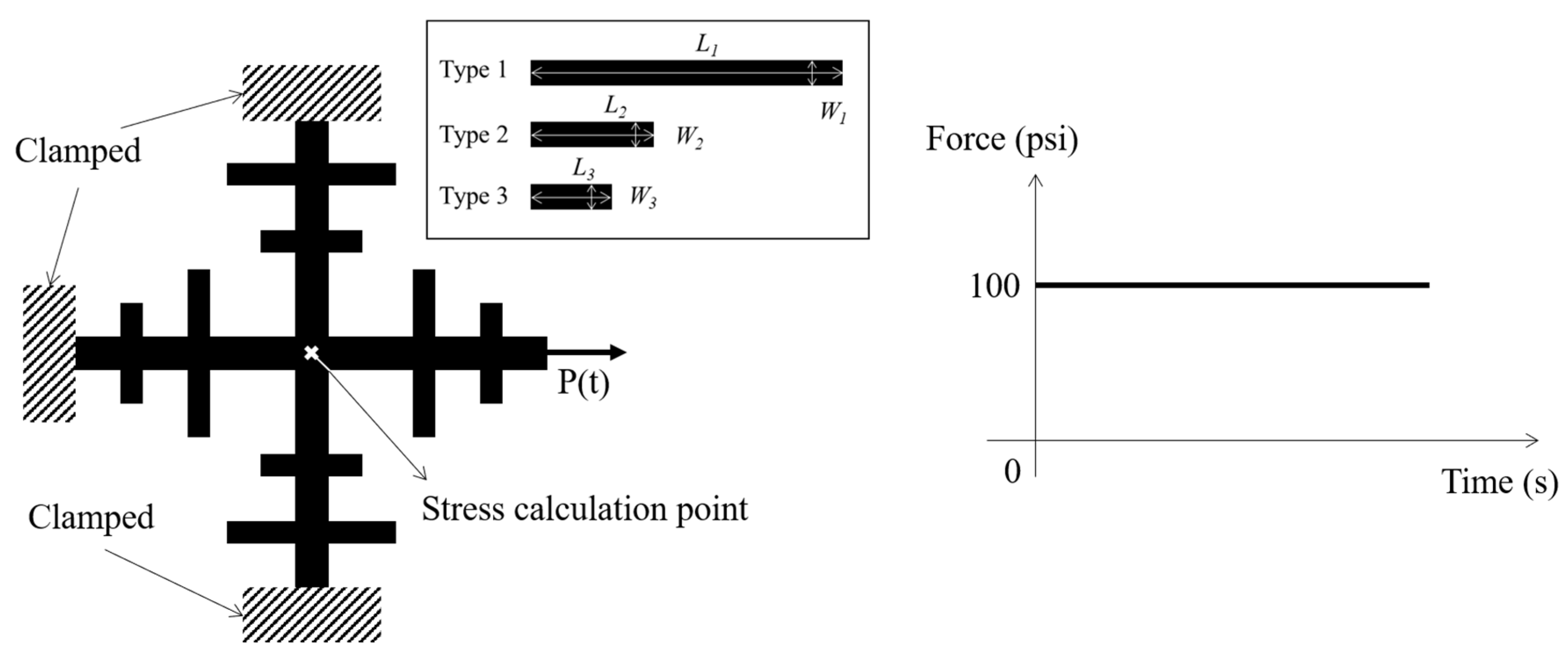
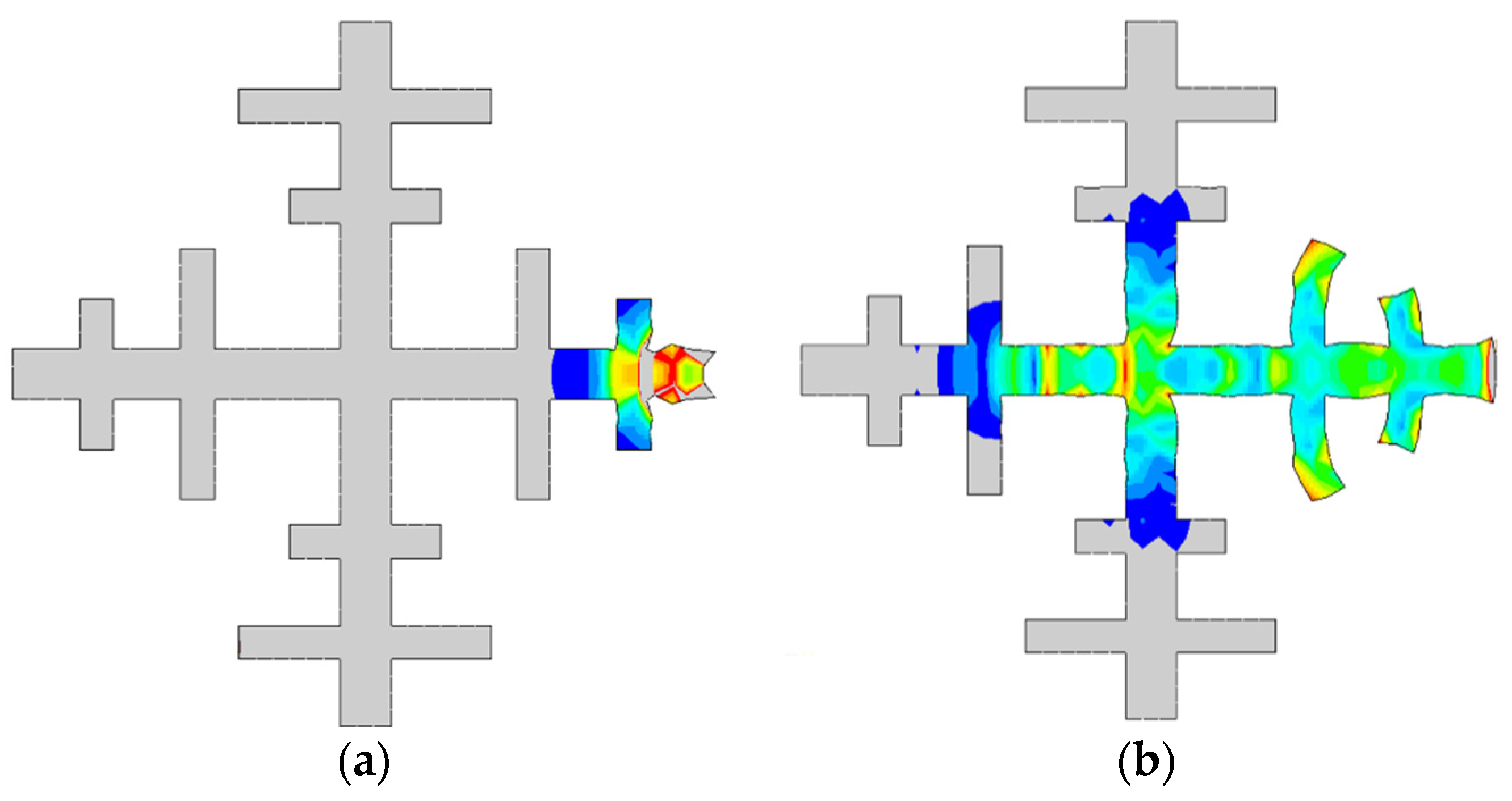
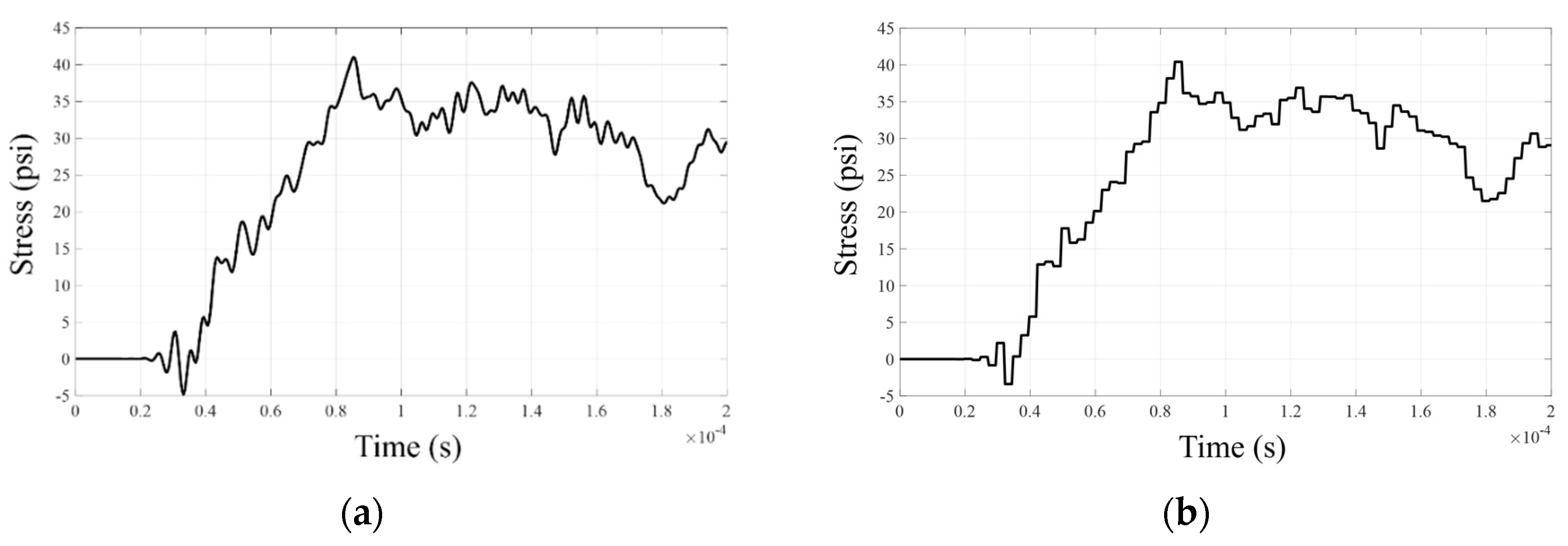
4. Numerical Examples

This section illustrates examples to demonstrate the benefits of the RFM in terms of accuracy as well as its limitations.
Example 1
Bar with three different segments
For the first example, a one-dimensional bar with different cross-section areas is considered. The problem geometry is composed of three different segments, as shown in Figure 8a, and each segment has a different cross-sectional area: 0.5 × 1 , 1.5 × 1 , and 0.5 × 1   in 2 , respectively. A step axial load of 100 psi in the x-direction is applied on the left side of the bar, and the example structure is discretized using 0.5   in × 0.5   in Q4 element meshes. The detailed geometry, boundary conditions, and material properties are illustrated in Figure 8.
Different from the previous benchmark example, the impedance mismatches at x = 8 and 11 in cause the occurrence of reflection and transmission waves owing to the change in the cross-sectional area. It should be noted that when a wave that propagates through a medium encounters the boundary of another medium having a different impedance, it produces reflection and transmission waves, as shown in Figure 9 [27].
The wave propagation impedance, Z, transmission coefficient, T, and reflection coefficient, R, can be defined by the following equations:
Z = p v ,
T = 2 Z 2 Z 2 + Z 1 = 2 1 + Z 1 / Z 2 ,
R = Z 2 Z 1 Z 2 + Z 1 = 1 Z 1 / Z 2 1 + Z 1 / Z 2 ,
where p and v denote the pressure (stress) and velocity vectors of the wave propagation, respectively. The transmission coefficient, T, and reflection coefficient, R, have the following relationship:
1 + R = T .
Based on Equations (35)–(38), the values for each coefficient can be obtained in this example. First, the impedance of Domain 1 and Domain 3 is three times greater than that of Domain 2. The transmission coefficients of the ( + ) x   d i r wave are 1/2 and 3/2 at x = 8   in and x = 11   in , respectively, and the reflection coefficient can be obtained from (37) accordingly ( R x = 8   in = 1 / 2 , R x = 11   in = 1 / 2 ). In the same way, the transmission and reflection coefficients for the ( ) x d i r wave can also be obtained. The analytical stress value at x = 9.75   in can be obtained through a step-by-step procedure, as shown in Figure 10.
Figure 11a shows the differences between the numerical solution and the analytical solution before applying the RFM, while Figure 11b–d shows the shape of the filtered numerical solution as the filtering length of the RFM changes. The shape of the filtered numerical solution changes according to the size of the filtering length of the RFM. The filtered numerical solution gradually becomes increasingly similar to the analytical solution as the filtering length increases. In addition, it can be confirmed that, in this example, the oscillation of the numerical solution decreases or disappears with the application of the RFM. However, the larger filtering length does not always guarantee better accuracy improvement (see Table 4). It should be noted that the RFM also plays an important role in the frequency domain. To explain this, the frequency components of the numerical solution without the RFM and analytical solution are presented in Figure 12.
Figure 12 shows that there is an enormous difference between the frequency components of the analytical solution and the numerical solution without the RFM. In particular, the analytical solution contains all of the frequency components, whereas the numerical solutions contain only the low-frequency components. Generally, a finer sampling time is required to consider higher frequencies, thereby increasing the computational cost. However, even finer sampling does not always guarantee inclusion of the higher-frequency components that appear in the analytical solution, as shown in Figure 12. In this study, however, it was discovered that a higher frequency range can be covered by using the RFM without modification of the sampling time.
As shown in Figure 13a, when the RFM is not applied, only the low-frequency components are present (black line). However, with the current RFM, several high-frequency components are generated (red line). In addition, increasing the filtering length creates additional new frequency components (see Figure 13b), and if the filtering length is greater than a certain length (in this example, greater than 8), the filtered numerical solutions can expand to cover all the frequency components (see Figure 13c). Note that the frequency components of the filtered numerical solution are changed without changing the sampling time. In general, the frequency components of the numerical solution are affected by the sampling time in a discrete system. In other words, with a chosen sampling time, the higher-frequency component is also determined. Applying the RFM can increase the higher frequency, which cannot be obtained by changing the sampling time.
Example 2
Complex geometric example
As the second example, Figure 14 considers a structure with many branches. Each bar has the same material properties as the previous problems: E = 30 × 10 6 psi, ρ = 7.4 × 10 4 lb-s2/in4, ν = 0 . A force is applied at the right arm, and the other arms are clamped. The stress at the center of the analysis domain is computed with and without the RFM.
Figure 14 shows the detailed shape of the complex beam structure with three types of rectangular beams. The example structure is discretized using 0.5   in × 0.5   in Q4 elements. It is not clear whether exact solution to this problem can be calculated. At least, we can find the shape of the wave propagation by the numerical method in Figure 15. The numerical solution and the results of applying the RFM to the numerical solution ( Δ t = 4.0 × 10 7   s ) are shown in Figure 16. As in the previous examples, spurious oscillation of the numerical solution is observed.
This time, the effect of the RFM with different filtering length, FL (not FR), is describe in Figure 16; Figure 17 to investigate feature of the RFM with respect to FL. In the frequency domain, the increase in the frequency components can be predicted by Theorem 1. For example, the noticeable frequency component of numerical (FEM) solution is distributed from 0 to 4 × 10 5 Hz, and we can expect an additional frequency component by RFM (FL = 2) as 8 × 10 5 to 12 × 10 5 Hz by Theorem 1: f ˜ = f s F L m ± f = 25 × 10 5 2 1 ± 4 × 10 5 . Without the RFM, the frequency components in the low-frequency region are dominant, whereas high-frequency components are generated with the RFM. This example shows that the RFM can work well even if the geometry of a structure is complex.

5. Conclusions

For future research, it is necessary to conduct a theoretical study to reveal a reasonable filtering ratio as well as a reasonable filtering length.
In numerical integration, the transient solutions of Newton’s second law obtained through either the implicit or explicit method inevitably exhibit undershooting or overshooting phenomena. Although both the stability and accuracy of the numerical methods are important, it is rare to investigate the accuracy of the time integration scheme compared with the stability issue. Thus, these numerical discrepancies are often neglected through the safety factor in mechanical or civil engineering. As a remedy for these discrepancies, this study develops an RFM for averaging the mechanical stress values in the time domain that improves the accuracy of the numerical solution. The RFM is a simple post-process averaging method to filter out the oscillations observed in the numerical solution and makes piecewise constant solutions of wave propagation problems. The performance of the present RFM was tested in both space and time with both the explicit and the implicit integration method. It was empirically found that a filtering ratio, FR, around 2% can improve the accuracy of numerical solutions. In addition, the frequency response functions for stress values before and after RFM application show that higher-frequency signals are added after filtering by generating piecewise constant responses. These higher frequency signals are essential to represent ramp phenomena in time domain. Though some benchmark problems, these higher-frequency components were investigated. One of the limitations of the present study is that it cannot provide the optimum filtering length for generalized wave propagation problems by a rigorous mathematical verification. In the same way, if the FR is too small it would not get rid of the oscillations, while if too large it would give big chunks of the solution into constant. By adopting a proper filtering ratio (around 2%) for the averaging operator in the RFM, it was observed that the averaged stress values converge toward the analytical stress values. For future research, it is necessary to conduct a theoretical study to reveal a reasonable filtering ratio as well as a reasonable filtering length.

Author Contributions

H.S.K., carries out the research and makes the computational codes; J.W.L., contributes to make the initial research codes and examples; K.K., provides the theorem; G.H.Y., provides key idea and conducts the studies. All authors have read and agreed to the published version of the manuscript.

Funding

This work was supported by the National Research Foundation of Korea (NRF) grant funded by the Korea government (MSIT) (No.2018R1A5A7025522) and was supported by the research program of Dongguk University, 2020.

Conflicts of Interest

The authors declare no conflict of interest

References

  1. Kolsky, H. Stress waves in solids. J. Sound Vib. 1964, 1, 88–110. [Google Scholar] [CrossRef]
  2. Kang, W.J.; Huh, H. Crash Analysis of Auto-Body Structures Considering the Strain-Rate Hardening Effect; SAE International: Warrendale, PA, USA, 2000. [Google Scholar]
  3. Bathe, K.-J. Finite Element Procedures; Prentice Hall: Upper Saddle River, NJ, USA, 2006. [Google Scholar]
  4. Bathe, K.-J.; Noh, G. Insight into an implicit time integration scheme for structural dynamics. Comput. Struct. 2012, 98, 1–6. [Google Scholar] [CrossRef]
  5. Cook, R.D. Concepts and Applications of Finite Element Analysis; John Wiley & Sons: Hoboken, NJ, USA, 2007. [Google Scholar]
  6. Logan, D.L. A First Course in the Finite Element Method; Cengage Learning: Boston, MA, USA, 2011. [Google Scholar]
  7. Kolsky, H. Stress Waves in Solids; Courier Corporation: Chelmsford, MA, USA, 1963; Volume 1098. [Google Scholar]
  8. Givoli, D.; Harari, I. Special issue on new computational methods for wave propagation. Wave Motion 2004, 4, 279–280. [Google Scholar] [CrossRef]
  9. Cho, S.; Huh, H.; Park, K. A time-discontinuous implicit variational integrator for stress wave propagation analysis in solids. Comput. Methods Appl. Mech. Eng. 2011, 200, 649–664. [Google Scholar] [CrossRef]
  10. Chung, J.; Hulbert, G.M. A Time Integration Algorithm for Structural Dynamics With Improved Numerical Dissipation: The Generalized-α Method. J. Appl. Mech. 1993, 60, 371–375. [Google Scholar] [CrossRef]
  11. Reed, W.H.; Hill, T. Triangular Mesh Methods for the Neutron Transport Equation; Los Alamos Scientific Lab.: Los Alamos, NM, USA, 1973.
  12. Hughes, T.J.; Hulbert, G.M. Space-time finite element methods for elastodynamics: Formulations and error estimates. Comput. Methods Appl. Mech. Eng. 1988, 66, 339–363. [Google Scholar] [CrossRef]
  13. Hulbert, G.M.; Hughes, T.J. Space-time finite element methods for second-order hyperbolic equations. Comput. Methods Appl. Mech. Eng. 1990, 84, 327–348. [Google Scholar] [CrossRef] [Green Version]
  14. Arnold, D.N.; Brezzi, F.; Cockburn, B.; Marini, L.D. Unified analysis of discontinuous Galerkin methods for elliptic problems. Siam J. Numer. Anal. 2002, 39, 1749–1779. [Google Scholar] [CrossRef]
  15. Huang, H.; Costanzo, F. On the use of space–time finite elements in the solution of elasto-dynamic problems with strain discontinuities. Comput. Methods Appl. Mech. Eng. 2002, 191, 5315–5343. [Google Scholar] [CrossRef]
  16. Ham, S.; Bathe, K.-J. A finite element method enriched for wave propagation problems. Comput. Struct. 2012, 94, 1–12. [Google Scholar] [CrossRef] [Green Version]
  17. Noh, G.; Bathe, K.-J. An explicit time integration scheme for the analysis of wave propagations. Comput. Struct. 2013, 129, 178–193. [Google Scholar] [CrossRef]
  18. Mullen, R.; Belytschko, T. Dispersion analysis of finite element semidiscretizations of the two-dimensional wave equation. Int. J. Numer. Methods Eng. 1982, 18, 11–29. [Google Scholar] [CrossRef]
  19. Krenk, S. Dispersion-corrected explicit integration of the wave equation. Comput. Methods Appl. Mech. Eng. 2001, 191, 975–987. [Google Scholar] [CrossRef]
  20. Christon, M.A. The influence of the mass matrix on the dispersive nature of the semi-discrete, second-order wave equation. Comput. Methods Appl. Mech. Eng. 1999, 173, 147–166. [Google Scholar] [CrossRef]
  21. Idesman, A.; Schmidt, M.; Foley, J. Accurate finite element modeling of linear elastodynamics problems with the reduced dispersion error. Comput. Mech. 2011, 47, 555–572. [Google Scholar] [CrossRef]
  22. Guddati, M.N.; Yue, B. Modified integration rules for reducing dispersion error in finite element methods. Comput. Methods Appl. Mech. Eng. 2004, 193, 275–287. [Google Scholar] [CrossRef]
  23. Idesman, A.; Samajder, H.; Aulisa, E.; Seshaiyer, P. Benchmark problems for wave propagation in elastic materials. Comput. Mech. 2009, 43, 797–814. [Google Scholar] [CrossRef]
  24. Holmes, N.; Belytschko, T. Postprocessing of finite element transient response calculations by digital filters. Comput. Struct. 1976, 6, 211–216. [Google Scholar] [CrossRef]
  25. Pryor, R.W. Multiphysics Modeling Using COMSOL®: A First Principles Approach; Jones & Bartlett Publishers: Burlington, MA, USA, 2009. [Google Scholar]
  26. Stolarski, T.; Nakasone, Y.; Yoshimoto, S. Engineering Analysis with ANSYS Software; Butterworth-Heinemann: Oxford, UK, 2018. [Google Scholar]
  27. Davison, L. Fundamentals of Shock Wave Propagation in Solids; Springer Science & Business Media: Berlin, Germany, 2008. [Google Scholar]
Figure 1. Response filtering method (RFM) concept.
Applsci 10 09032 g001
Figure 2. Illustration of the mechanical stress wave problem: (a) the problem definition in [5], and (b) the force condition.
Applsci 10 09032 g002
Figure 3. Comparison of the mechanical stresses at x = 9.75 (20th element) for the benchmark problem in Figure 2.
Applsci 10 09032 g003
Figure 4. Comparison between the exact (analytical) solution and the filtered numerical solution (Left: central-difference method, Right: Newmark’s method). The responses are shown (a) without RFM, (b) with FR = 0.5%, (c) with FR = 1%, and (d) with FR = 2%.
Applsci 10 09032 g004aApplsci 10 09032 g004b
Figure 5. Comparison of the mechanical stresses at x = 0.25   in (1st element) for the benchmark problem in Figure 2.
Applsci 10 09032 g005
Figure 6. Modification of the original signal depending on the filtering length (FL): (a) without RFM, with RFM for (b) FL = 2, (c) FL = 4, and (d) FL = 5.
Applsci 10 09032 g006
Figure 7. Changes to the numerical solution (Newmark’s method) in frequency domain after filtering with different filtering ratio and comparison with the exact solution for benchmark problem in Figure 2. (a) Numerical solution without RFM, (b) with RFM (FR = 0.5%), and (c) with RFM (FR = 2%).
Applsci 10 09032 g007aApplsci 10 09032 g007b
Figure 8. Geometric parameters of Example 1 (a) The problem definition ( L 1 = 8   in , L 2 = 3   in , L 3 = 9   in , h 1 = 0.5   in , h 2 = 1.5   in , h 3 = 0.5   in , and Thickness = 1   in ), and (b) the force condition.
Applsci 10 09032 g008
Figure 9. Transmission wave (subscript t) and reflection wave (subscript r) of an incident wave (subscript i) perpendicular to the boundary between two media.
Applsci 10 09032 g009
Figure 10. Schematic diagram of the analytical solution.
Applsci 10 09032 g010
Figure 11. Changes before and after filtering with different filtering lengths and comparison with the analytical solution for Example 1: (a) without filtering, (b) with FR = 0.5%, (c) with FR = 1%, and (d) with FR = 2%.
Applsci 10 09032 g011aApplsci 10 09032 g011b
Figure 12. Decomposition of the analytical solution and the numerical solutions without RFM in the frequency domain for Example 1.
Applsci 10 09032 g012
Figure 13. Changes to the numerical solution after filtering with different filtering ratio and comparison with the analytical solution for Example 1 in the frequency domain: (a) filtered solution with FR = 0.5%, (b) with FR = 1%, and (c) with FR = 2%.
Applsci 10 09032 g013
Figure 14. Example 2: problem geometry, boundary conditions, and force condition ( L 1 = 21.5   in ,   L 2 = 7.5   in ,   L 3 = 4.5   in ,   W 1 = 1.5   in ,   W 2 = W 3 = 1   in , thickness = 1   in ).
Applsci 10 09032 g014
Figure 15. Shape of wave propagation viewed through the von Mises stress and deformation for Example 2 (Ansys 19.0 stress contour package). The illustration of wave propagation is shown at (a) t = 1.85 × 10 5 and (b) t = 1.4 × 10 4   s .
Applsci 10 09032 g015
Figure 16. Changes before and after filtering with different filtering lengths: (a) without filtering, (b) with FL = 2, (c) with FL = 4, and (d) with FL = 8.
Applsci 10 09032 g016aApplsci 10 09032 g016b
Figure 17. Changes in the numerical solution after filtering with different filtering lengths in the frequency domain (the dashed and solid lines represent the numerical solution without RFM and filtered numerical solution, respectively): (a) direct numerical solution, filtered solution (b) with FL = 2, (c) with FL = 4, and (d) with FL = 8.
Applsci 10 09032 g017
Table 1. (a) Accuracy improvement of the RFM with different numerical integration method ( at   20 th   element ,   Δ t = Δ t 1 = 4.0 × 10 7 s ). (b) Accuracy improvement of the response filtering method with different numerical integration method ( at   20 th   element ,   Δ t = Δ t 1 × 10 1 s ).
(a)
Central-difference method
Filtering ratio (%) w/o RFM0.511.522.533.5
Error indicator ξ ( × 10 3 ) 1.84721.82831.70971.59671.38081.21241.22411.1895
Number of over (under) shoots6765584528211919
Newmark’s method
Filtering ratio (%) w/o RFM0.511.522.533.5
Error indicator ξ ( × 10 3 ) 1.72231.70531.59411.43871.31231.12051.19371.1340
Number of over (under) shoots6565654927202019
(b)
Central-difference method
Filtering ratio (%) w/o RFM0.511.522.533.5
Error indicator ξ ( × 10 3 ) 1.78831.75391.65431.49681.30461.36401.21361.0409
Number of over (under) shoots6564594126191917
Newmark’s method
Filtering ratio (%) w/o RFM0.511.522.533.5
Error indicator ξ ( × 10 3 ) 1.78761.75151.65101.49621.30641.36181.21651.0495
Number of over (under) shoots6564594126191917
Table 2. Accuracy improvement of the RFM with different numerical integration method ( at   1 st   element ,   Δ t = 4.0 × 10 7 s )
Central-difference method
Filtering ratio (%) w/o RFM0.511.522.533.5
Error indicator ξ ( × 10 3 ) 1.67101.64001.50391.37231.09181.10120.96660.9809
Number of over (under) shoots7373734719152323
Newmark’s method
Filtering ratio (%) w/o RFM0.511.522.533.5
Error indicator ξ ( × 10 3 ) 1.60251.58111.42691.33391.17460.97520.98270.9688
Number of over (under) shoots7171715121132123
Table 3. Generated frequencies predicted using Theorem 1: 0 f ˜ f s 2 ( N = 100 , T 0 = 0.1   s , f s = N T 0 = 1000   Hz ).
Filtering   Length   ( F L ) Generated   Frequencies   ( f ˜ )
150 Hz
250 Hz, 450 Hz
450 Hz, 200 Hz, 300 Hz, 450 Hz
550 Hz, 150 Hz, 250 Hz, 350 Hz, 450 Hz
Table 4. Accuracy improvement of the RFM with varying filtering length in Example 1.
Newmark’s Method
Filtering ratio (%) w/o RFM0.511.522.533.5
Error indicator ξ ( × 10 3 ) 2.56222.54632.47122.38832.33302.04532.00962.0617
Number of over (under) shoots4040403428222222
Publisher’s Note: MDPI stays neutral with regard to jurisdictional claims in published maps and institutional affiliations.

