Calibration of Reanalysis Data against Wind Measurements for Energy Production Estimation of Building Integrated Savonius-Type Wind Turbine

Abstract

In this work, a cost-effective wind resource method specifically developed for the ROSEO-BIWT (Building Integrated Wind Turbine) and other Building Integrated Wind Turbines is presented. It predicts the wind speed and direction at the roof of an previously selected building for the past 10 years using reanalysis data and wind measurements taken over a year. To do so, the reanalysis wind speed data is calibrated against the measurements using different kinds of quantile mapping, and the wind direction is predicted using random forest. A mock-up of a building and a BIWT were used in a wind tunnel to perform a small-scale experiment presented here. It showed that energy production is possible and even enhanced over a wide range of attack angles. The energy production estimations made with the best performing kind of calibration achieved an overall relative error of 6.77% across different scenarios.

1. Introduction

Small wind turbines are a useful technology for transitioning to a more sustainable energy model. They are a good way to decentralize electricity generation, an objective set by the European Union through its 2009/72/EC directive [1]. Among these, Building Integrated Wind Turbines (BIWT) are specially interesting for many reasons, such as:

• Since they are installed on buildings and can be installed within cities, which are both big energy consumers, transport and transformation losses are reduced.
• Being installed on already urbanized areas, they avoid some of the environmental [2] and social [3] impacts of conventional wind farms, such as land use, visual pollution of natural areas, and destruction or disruption of habitats.
• They can be installed alongside solar panels to create hybrid generation systems. Power generation becomes more stable compared to pure photovoltaic system of the same rated power. In isolated installations, this can lead to a lower set-up cost because less batteries are needed to ensure that demand is met [4].
• They can play a key role on the so called nearly Zero-Energy Buildings [5].

With the promotion of small wind turbines in mind, the authors of this paper have been working on a novel Savonious-type small wind turbine specifically designed for urban environments called ROSEO-BIWT, which has already been presented in previous papers [6,7]. We have the conviction that any small wind turbine has to be cost effective if it is going to contribute to the mentioned energy transition, and a proper wind resource assessment method is key for that [8].

Traditional wind farms require extensive monitoring and measurements plans. For instance, according to the National Renewable Energy Lab [9], a single measurement tower that takes wind and other variable readings costs about US$25,000 and US$40,000 to set up and maintain. A small wind turbine does not justify such an expensive and detailed analysis to spot a good location, or to calculate the potential of an already chosen location. Apart from that, the topography of the place has to be taken into account. Landberg et al. propose using CFD (Computational Fluid Dynamics) simulation for each site for this, but, as they note, it consumes a large amount of time and computing capacity [10].

The aim of this paper was to present a wind resource estimation method that requires few computational resources and that takes into account the particularities of our turbine, primarily being its high sensitivity to the wind direction and the concentrating effect of the building and the concentration panels. Furthermore, each aspect of this method can be applied to other small wind turbine designs. It estimates the energy production of a previously selected building, allowing for calculation of the return on investment. It also helps selecting the facade or facades most suitable for an installation. For this study, the specific case of the University of the Basque Country’s building in the town of Eibar was studied [11].

There have already been attempts to develop efficient methods for small wind turbines. Weekes et al. [12] suggests fitting linear functions that given the wind module speed of a reference site output the estimated module of a target site. This method has some inconveniences. First of all, it can predict negative wind speed values at the target side because of the residual scatter term. The authors solved this by setting the negative predicted values to the mean of the function before applying that term. However, this could lead to overestimating the wind potential at the target site. The second inconvenient is that a linear regression escalates the whole wind speed range with the same factor: the slope of the linear function. This means that non-linear effects cannot be properly taken into account.

Instead of this, we propose using quantile mapping to come with a similar method that does not have such inconveniences and that is specially suitable to get the overall potential of a site. This technique consists in training transference functions that match the quantiles of a forecast sample with the quantiles of an observation sample. Then, those functions can be used to come up with forecasts when observations are not available. Apart from its extensive use in the field of meteorology, it has already been used in the context of wave [13,14,15], solar [16,17], and wind energy [18,19,20].

In the method presented in this paper, reanalysis data is used as observation and wind measurements data as forecast. The goal is to get a calibrated time series of the wind speed module of several years of a site even if measurements were only taken for a much shorter time period. That way, the energy potential estimation is not affected by the peculiarities of the measurement period. For this purpose, the calibrated data does not need to be a precise forecast; instead, it has to match the probability distribution of the wind speed module time series of a typical year.

2. Data and Methodology

Due to the complexity of the methodology, the diagram shown in Figure 1 was made. It shows the process by which the best predictive models were chosen, but it does not cover its application to the 10-year data period that gives us the results in Section 3.4.2.

2.1. Data

2.1.1. Anemometer Data

The measurements were taken at the roof of the University of the Basque Country’s building in Eibar, located at the following coordinates: 43${}^{°}$10${}^{\prime }$45.82${}^{″}$ N, 2${}^{°}$29${}^{\prime }$19.80${}^{″}$ W. A cup and vane anemometer was used. It measured the wind speed in intervals of approximately 7 min and uploaded the mean wind speed and the direction of each interval to a web page. The data could later be retrieved using web scrapping techniques. A year of data was used, covering the period from the 22nd of May 2018 to the same day of 2019. This way, the effect of the changing weather during the year could be taken into account, without having an excessively long measurement period that would make the method unattractive for commercial use.

Ideally, if one of the facades of the building was already selected, the anemometer would have been installed on the edge between that facade and the roof, where a turbine would be installed. Alternatively, it could be installed on the center of the roof, which would allow to select the facade taking the measurements into account. However, due to architectonic and legal limitations, none of these options were possible, and the anemometer had to be installed on one side of the roof several meters away from the edge.

The anemometer’s data was filtered to ensure that all measurements used in the calibration were taken while the anemometer was working properly. These filters detected suspicious measurements but did not automatically delete them. Instead, the positions of those measurements were stored, so they could be plotted later, along with all the data. That way, the proper functioning of the filters could be checked, and their parameters could be tuned, before deleting any data. Three of them were used:

1.

The first filter detected measurements with negative wind speed or values greater than 30 m/s.

2.

The second one detected if the difference between two subsequent measurements was greater than 5 m/s.

3.

The third one detected whether 20 subsequent measurements varied their mean wind speed less than 0.05 m/s.

When applying these filters, the first one did not detect any errors, the second one detected 3, and the third one detected 117. Overall, a 0.12% of the data points were flagged as erroneous and deleted, so the filters did not meaningfully affect the data set.

2.1.2. Reanalysis Data

The reanalysis data used in this study came from the ERA5 hourly data (ERA5 from now on) provided by the European Center for Medium-Range Weather Forecasts. It has a temporal resolution of one hour and a spatial one of 0.1${}^{°}$, and it contains values of multiple variables for each hour and grid point [21].

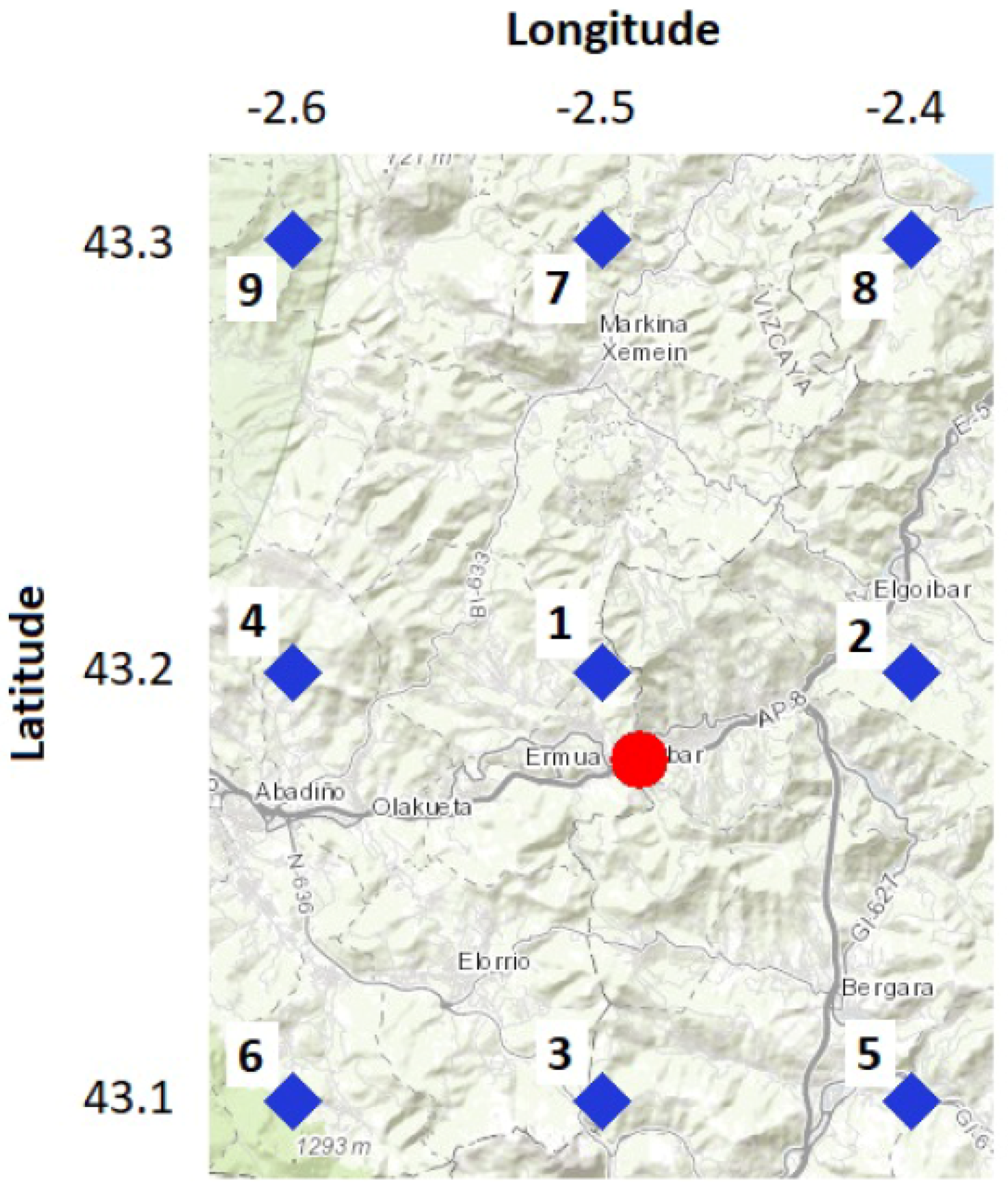
The ERA5 data used in this study covers 10 years, from 2010 to 2019, both included. The 9 grid points closest to the anemometer were selected. As seen in Figure 2, they form a $3\times 3$ square around the town of Eibar, being the one in the center the closest to the anemometer.

From all available variables, the 10-m and 100-m components of wind were used. The wind speed module and direction were calculated from these components, so the ERA5 data would be similar to the anemometer’s.

2.1.3. Data Merging and Cross-Validation

Since the reanalysis data’s time period totally overlaps the period in which the measurements were taken, it is possible to merge both data sets (ERA5 data and the measurements) to form another one that covers that time period. It was done in a way that every data point corresponded to a timestamp and had the wind speed modules and directions of the anemometer and the reanalysis. Since ERA5 data had the lowest sampling frequency, every measured speed and direction was matched with the ERA5 data point that was closest in time, and all other measurements were discarded.

The anemometer took a sample every 7 min when working properly, so, in most of the final data set, the ERA5’s and the anemometer’s timestamps of each data point were no more than 3.5 min apart. However, the gaps in the anemometer’s time series could theoretically mean that some ERA5 data points could be matched with measurements taken a long time apart, or that various of them were matched with the same measurement. Those mismatched data points could disrupt the calibration, but luckily none of the gaps was large enough to do so, as the biggest difference between the anemometer’s and ERA5’d timestamp for the same data point was around 5 min. This meant that, in this particular case, no data points were discarded.

In order to cross-validate the results, this data set was randomly split in two equal-size sets: one for training and the other one for testing. The splitting was made just once for the whole study; that means that all the quantile mapping calibrations, the classification via random forest, and the estimation of produced energy done on the 1-year data set were trained and tested with the same training and testing data sets.

By this point, we have three different data sets that contain timestamps and wind speed and direction data.

Table 1. Summary of the scope of each data set.

	Anemometer Data	Reanalysis Data	Merging of Both Anemometer and Reanalysis Data
Spatial (number of sites)	1	9	10
Temporal (years)	1	10	10
Height	Rooftop	10 m and 100 m	Rooftop and 10 m

below shows the scope of each data set for clarification purposes.

2.2. Interaction between Wind Direction and Building Orientation

2.2.1. The Importance of the Skew Angle and a Small-Building Experiment

The skew angle of any Vertical Axis Wind Turbine (VAWT) is the angle between the plane perpendicular to the rotation axis and the incoming wind direction, which means that, for a regular VAWT, it has a value of zero when the wind only has horizontal components, as well as a value of 90${}^{°}$ when it has only vertical ones. If the VAWT is mounted horizontally on the edge between the roof and the facade, this is the same angle as the angle between the plane perpendicular to both the facade and the roof and the wind direction. When working with wind turbines in this position, it is very important to take this angle into account when estimating the wind resource because they only work when the wind is facing the facade.

To determine the maximum skew angle with which the turbine can generate the potency given by the power curve for a particular wind speed, a small wind tunnel experiment was run. It involved using a mock-up of a building with a miniature Savonious turbine and Power Augmenting Guiding Vanes (PAGVs). The turbine was attached to a dynamo, from which voltage readings were taken. The voltage was later used to calculate the rotation speed for each wind speed and skew angle.

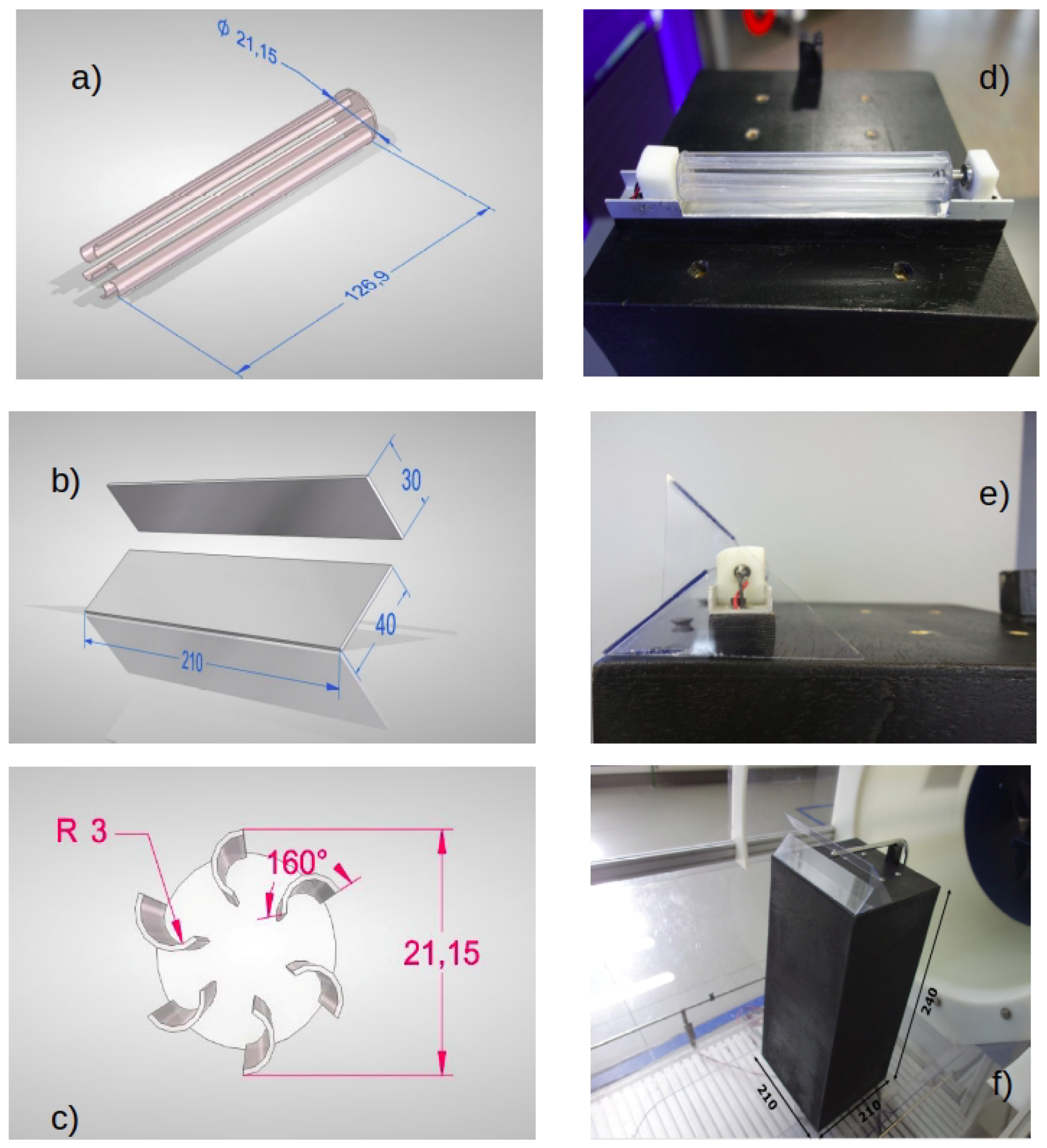
Figure 3 shows the design, dimensions, and photos of the small-scale model with a 6-bladed small turbine within the PAGVs and the building. Figure 3a,d shows the first design and the corresponding real construction of the small turbine along the building (plant view). The profile of the design and real methacrylate PAGVs are shown in Figure 3b,e. Figure 3c’s profile view shows the design and exact dimensions and angles of the 6 blades, while Figure 3f is a photo of the small building with the PAGVs in a previous experiment.

The electrical motor attached to the small turbine is a maxon DCX06M EB KL 6V of 0.529 W (speed constant of 3060 min${}^{-1}$ V${}^{-1}$, speed–torque relation of 36,600 min${}^{-1}$ m Nm${}^{-1}$). This description and the characteristics of the wind tunnel in which the skew angle experiment is performed are already described in our previous publication [7]. Although the blockage ratio of the small scale experiment (the transverse area of the small building with respect to the wind tunnel circular area) should be below 10% [22], a blockage ratio of around 20% is obtained even with our precise scale model of the turbine. In the future, a bigger wind tunnel in necessary with a wider range of wind speeds.

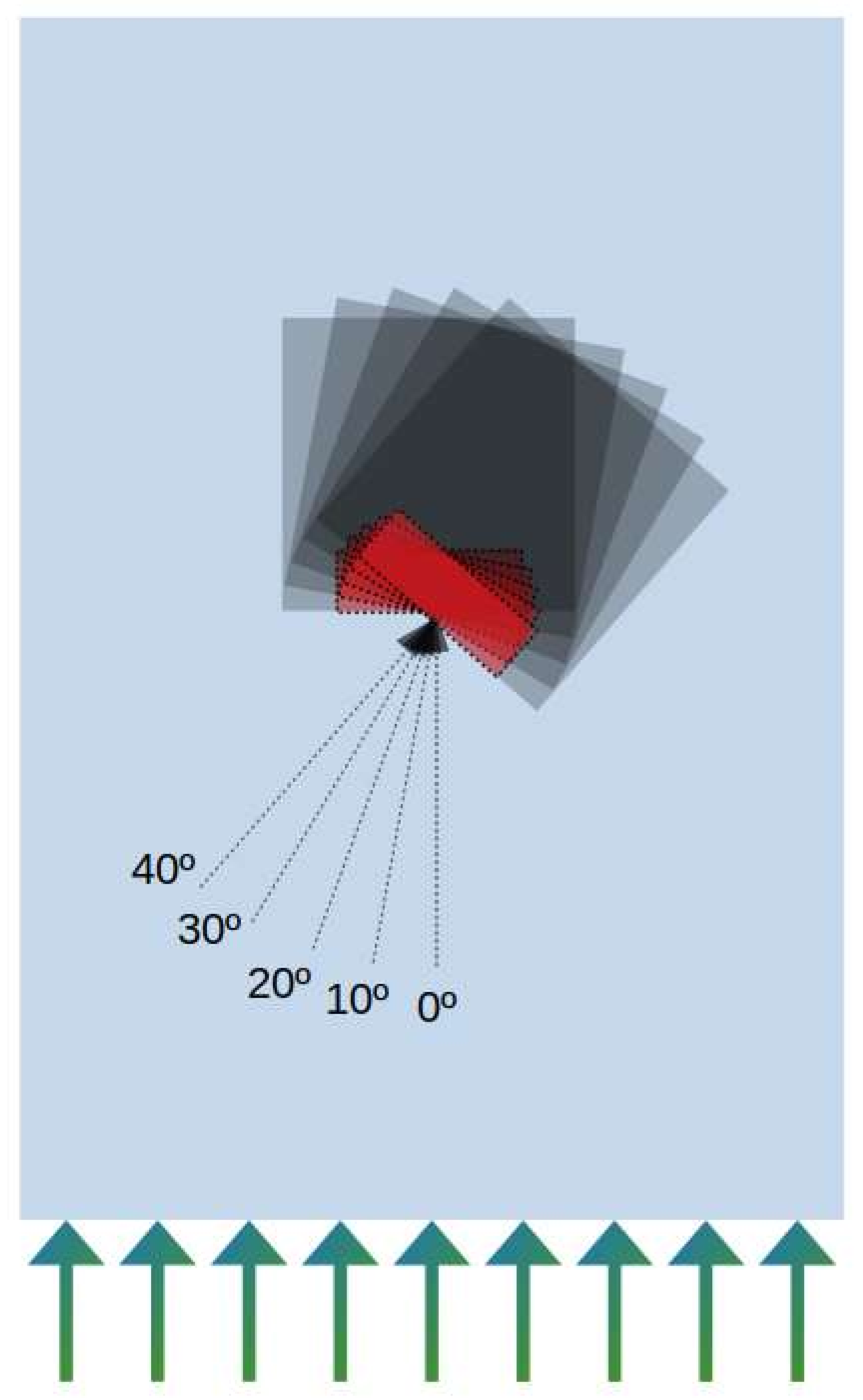
Although the experiment is preliminary and should be validated by CFD or in a bigger wind tunnel, it shows very relevant results for our purpose and the configuration of our Savonius turbine. It should be noted that the horizontal plane skew angle with respect to this horizontally mounted Savonius is analogous to the typical vertical plane skew angle with respect to a VAWT (see Figure 4). The experiments were developed for wind speeds around 6 m/s, 7 m/s, and 8 m/s. There are fluctuations in the measured wind speed and the rotational speed (rpm) of the small Savonius, and that is why boxplots are used for the representation of the graph.

Figure 5 shows the behavior of the small turbine for different skew angles (0${}^{°}$, 10${}^{°}$, 20${}^{°}$, 30${}^{°}$, and 40${}^{°}$), with the 0${}^{°}$ being the angle corresponding to perpendicular wind to the facade (pink color). The skew angle deviation, surprisingly, does not affect the measured $rpm$; they even increase for higher skew deviations from the perpendicular incidence.

A hypothesis on this anti-intuitive behavior can be related to the helical rotative wake or vortex prolonged along the horizontal axis, the energy of which is not dissipated and is captured by the turbine. This idea should be validated by more detailed CDF simulations than previous works [23], but other authors have also observed also this behavior of the Savonius and other VAWTs’ power production with respect to the skew angle even with higher $C_{p,max}$ values for non-skewed cases [24,25,26].

2.2.2. Selection of Facade for Installation

After reassuring that this kind of turbine can work with a wide range of wind directions, we can now examine the wind resource on the building’s roof. With this information, the best facade or facades can be selected, and, after that, the hypothetical wind energy output of a installation on that or those facades can be estimated.

For this purpose and for simplicity’s sake, we will suppose that the $C_{p,max}$ does not increase nor decrease from 0${}^{°}$ to 60${}^{°}$ of skew angle, as well as that it drops to zero with higher values. This is consistent with the tendency found at the wind tunnel experiment explained in the previous Section 2.2.1, as well as with Reference [25]. This means that, in our analysis, a turbine mounted between the roof and a facade absorbs the wind coming from a range of 120${}^{°}$ in front of the facade.

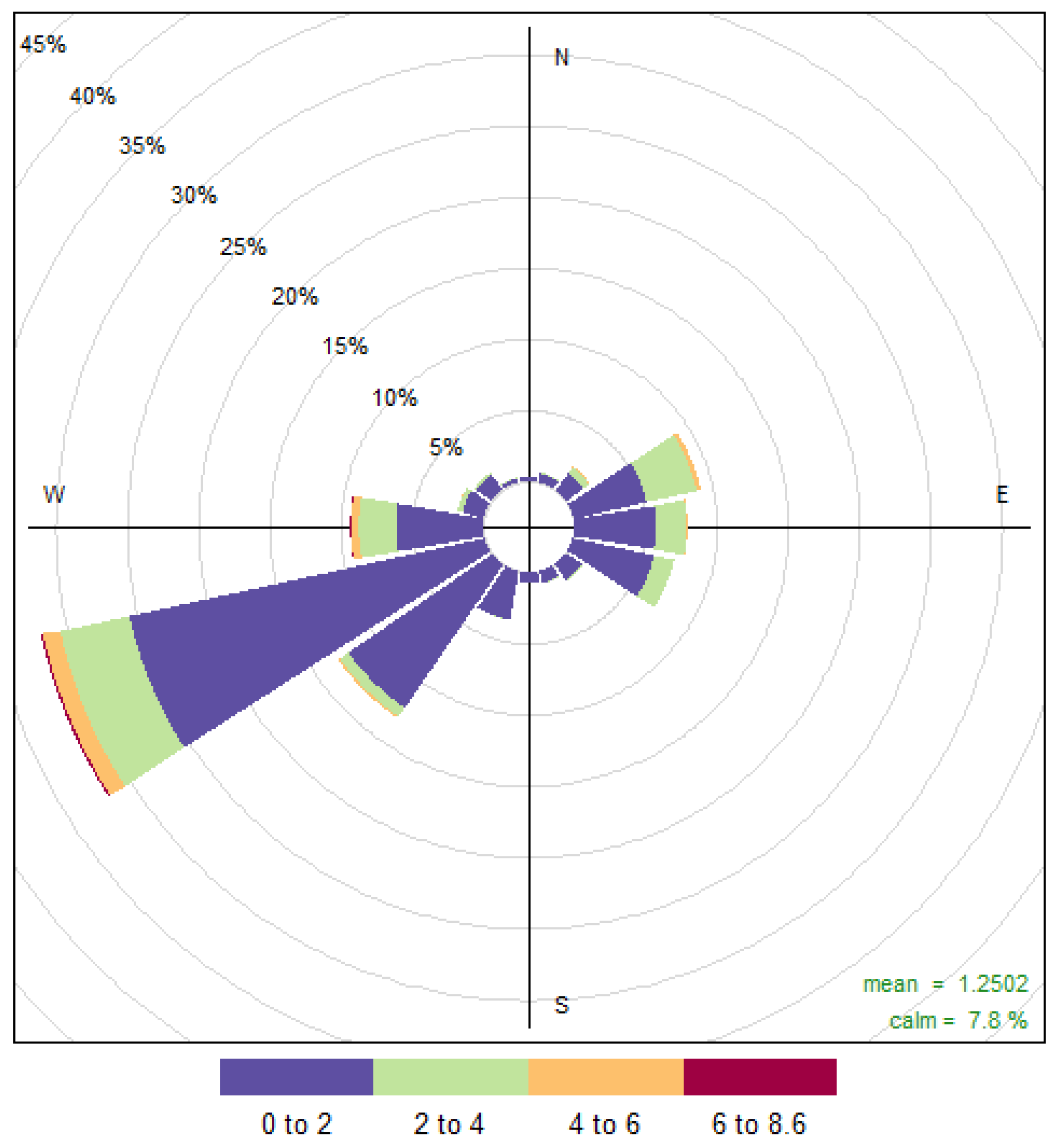
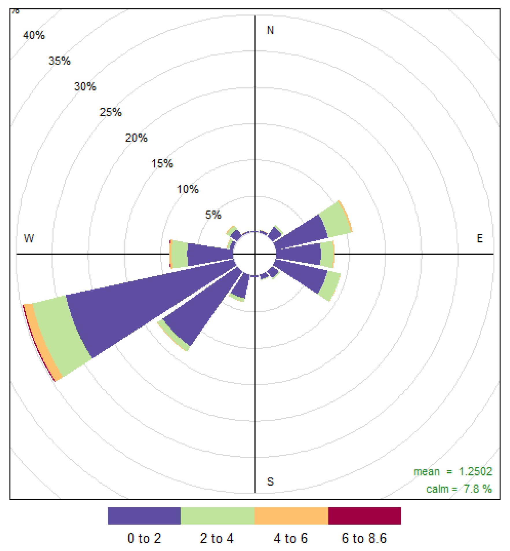
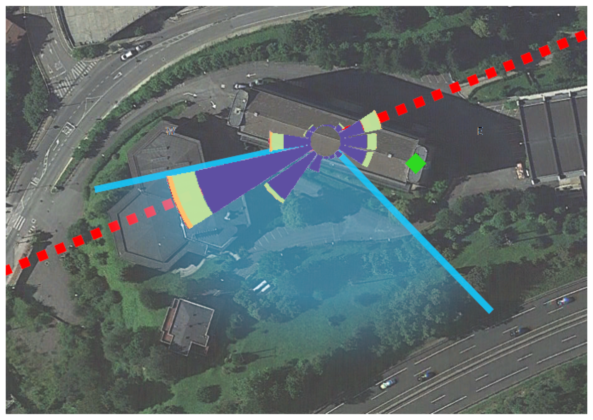
After studying the wind rose of the wind measurements taken on the building, it is very clear that the valley in which the town of Eibar is located concentrates the wind, since the predominant wind directions are the ones parallel to the valley’s direction. This means that the building primarily receives wind from the NE and specially the SW, as seen in Figure 6. Even if various facades could be selected to augment the overall produced energy, selecting only the best facade is the best option for optimizing the capacity factor and thus making the installation more economically viable. Apart from that, wide facades are desirable over narrow ones because they concentrate the wind better and because they give more room for the installation. For all these reasons, the south facade was selected. This facade directly faces the wind coming from 197${}^{°}$, so the absorption range covers any wind coming from 137${}^{°}$ to 257${}^{°}$. Figure 7 shows that the 120${}^{°}$ range is wide enough to absorb the strongest winds.

2.3. Calibrations via Quantile Mapping

Once the training and testing data sets were ready, the measurements were calibrated against the reanalysis 10-m wind data using quantile mapping, quantile matching or QM. This technique seemed appropriate for energy output estimation purposes because it makes the PDF of the reanalysis data more akin to that of the measurements. It has already been used by the authors in a wider context of renewable energies, such as the study of historical wave energy trends in Ireland, Chile, or the Bay of Biscay [13,14,15,27], and by other researchers in the context of solar [16,17] and wind energy [18,19,20].

A first round of simple calibrations was performed for each of the ERA5 grid points using quantile mapping. We call them simple because they were not categorized, meaning that the training data set was not splitted, as opposed to the following calibrations. The results, which are more extendedly discussed in Section 3.1, showed that both ERA5’s and the calibrated wind speed did not show meaningful differences between grid points. For these reason and for simplicity’s sake, only the grid point closest to the anemometer was used for the next three calibrations. These are performed on categorized data sets, meaning that the training data set was split using different criteria and that the training and calibration process were done independently on each split. The first of them was directional, the second one seasonal, and the third one was both directional and seasonal; each one’s most distinguishing properties are summarized in

Table 2. Summary of the distinctive properties of the QM (Quantile Mapping) calibrations performed.

Name	Grid Points	Splitting Criteria	Splits
Simple	Closest 9	None	1
Directional	Closest one	ERA5 wind direction	8
Seasonal	Closest one	Season	4
Combined	Closest one	ERA5 wind direction & Season	8 × 4 = 32

for clarification purposes.

To perform the directional calibration, 8 wind directions were used, corresponding to the cardinal and intercardinal directions. All data points were grouped according to which of those directions were closer to their ERA5’s wind direction, and separate training and calibrations were done for each one. This way, the calibrations of the data points that had a ERA5 wind direction between established ranges were done using transference functions trained only with data points with a ERA5 direction within that range.

The seasonal calibration consisted of splitting the data set based on the season instead of the direction. For simplicity, instead of accurately grouping the data points according to seasons, they were grouped by months: the data from January, February, and March was considered as being part of “winter”; April, May, and June as “spring”; July, August, and September as “summer” and October, November, and December as “autumn”. Following the same logic as the directional calibration, the data from each season was trained and calibrated separately.

The third and last calibration was a combined calibration, meaning that it was directional and seasonal at the same time. The directions and seasons were the same as in the previous calibrations, so the data points were split in 32 groups, according to their ERA5 direction and season.

2.4. Adaptation of Calibrated Wind Speed Series to ROSEO-BIWT’s Peculiarities

2.4.1. Correction of Wind Speed Series

Due to architectonic and legal restrictions, the anemometer could not be located at the same spot as the hypothetical turbine. Instead of being on the edge between the roof and the center of the facade, where the concentrating effect of the building is more potent, it was installed over the roof on one side of the building, as shown in Figure 7. This caused the measured wind speed to be lower than what empirical observations suggested a hypothetical turbine could receive.

This was compensated by multiplying the wind speed series by a range of augmenting factors, which are the ratio between the mean wind speeds at the anemometer’s and the turbine’s locations. These were deduced from the findings of previous research done on the difference of the wind speed on the area around the roof relative to the free wind speed [24].

According to this paper, the installation site (that is, the spot just above the edge between the roof and the facade facing the wind) has wind speeds that are between 0.33 and 0.9 times the free wind speed. Our hypothesis is that this difference is constant for the entire wind speed range for a given building and facade. So, by knowing the mean wind speed value between the wind at the anemometer and the free wind, we can also calculate the factors. Since the free wind is the wind that occurs at such a height where it is no longer slowed down by the roughness of the terrain, the 100-m wind data from ERA5 was used as free wind.

They were calculated as follows: first, the data pertaining to the times when the wind was facing the selected facade (using the 120${}^{°}$ range explained in Section 2.2.2) was separated from the rest. Then, within this subset of data, the averages of the measured and ERA5’s 100 m wind speeds were calculated, and the former was divided by the latter. We will call this factor $f_a$, which is equal to 0.26.

Another factor, called $f_b$, represents the difference between the mean wind speeds at the edge and at 100-m height and can be extracted from the CFD simulation results of Micallef et al. [24]. In order to take into account different scenarios regarding the increase of the wind speed at the edge, three different values were used. We will call them $f_{b_1}$, $f_{b_2}$, and $f_{b_3}$, and their values are 0.33, 0.6, and 0.9, respectively.

Lastly, by dividing $f_b$ by $f_a$, we got what we will call $f_c$, which is the difference between the edge and the anemometer’s spot, that is, the correcting factors for the measured and calibrated wind speed series. Having different values for $f_b$ means that we got different values for $f_c$: $f_{c_1}$ is equal to 1.28, $f_{c_2}$ to 2.34, and $f_{c_3}$ to 3.50. The equations below summarize the calculations. $AnemWS$ is the mean wind speed value of the measured wind speed inside the absorption range, $FreeWS$ is the mean wind speed of the ERA5’s 100-m data pertaining to the same data points $AnemWS$, and $EdgeWS$ is the mean speed of the wind that, according to these calculations, the turbine would receive.

$$f_a=\frac{AnemWS}{FreeWS}=0.26,$$

$$f_b=\frac{EdgeWS}{FreeWS},$$

$$f_{b_1}=0.33,$$

$$f_{b_2}=0.6,$$

$$f_{b_3}=0.9,$$

$$f_c=\frac{f_b}{f_a}=\frac{EdgeWS\times FreeWS}{FreeWS\times AnemWS}=\frac{EdgeWS}{AnemWS},$$

$$f_{c_1}=1.28,$$

$$f_{c_2}=2.34,$$

$$f_{c_3}=3.50.$$

2.4.2. Prediction of Wind Direction via Random Forest

Since the direction from which the building receives the wind greatly affects the concentrating or obstructing effect of the building’s geometry, a method to predict the past wind direction is necessary in order to use historical data for wind resource estimation. The random forest (RF) algorithm was chosen for this task because of its ability to use different types of inputs and evaluate its relevance, so it can be fed with the historical reanalysis data already on hand without any previous variable selection. Apart from that, being an ensemble learning method means that it is more robust and less likely to overfitting than single decision trees.

Predicting a variable, such as the on-site wind direction, is tricky because it is a numerical cyclical variable. For instance, the values 360${}^{°}$ and 0${}^{°}$ refer to the same direction. However, the low resolution of the anemometer’s wind direction data, which only differentiates between 16 directions, means that it behaves more like an ordinal cyclical variable. Apart from that, there is no way that we are aware of to make a random forest predict a cyclical variable, be it numerical or ordinal. For that reason, the on-site wind direction variable is treated as categorical, even if it means some loss of information.

The reanalysis data used in the calibrations is used as input. Since the comparison of the grid points’ wind speed showed that they are very similar, only the wind speed of the closest point was used, while the 9 variables of wind direction were used. The month of each data point was also added as a predictor, since the seasonal calibration’s performance already showed that there are changes on the relationship between the modeled and the measured wind throughout the year. The month to which each data point corresponds is encoded as a categorical variable for the same reasons exposed for the on-site wind direction: few cases and cyclical nature.

That gives a total of 11 input variables to predict a categorical variable with 16 classes. The number of variables randomly sampled as candidates at each split was set to 3, following the advice given by Svetnik et al. [28], which states that this number should be set to the root square of the number of predictors. The number of trees for the RF was set to 500. The tuning and posterior use of the algorithm was made in a similar fashion to that of the calibrations: first, the tuning and validation were made using the training and testing data sets, respectively, and, once the correct parameters were found, an RF was generated without using cross-validation (that is, using both sets), and then it was used to predict the on-site wind direction for the period ranging from 2010 to 2019.

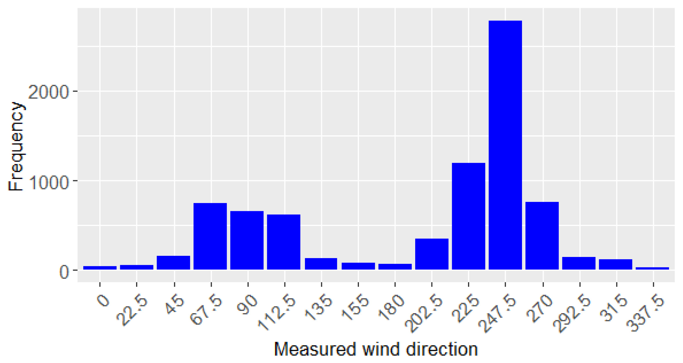
The tuning involved dealing with the unbalanced nature of the on-site wind direction, which the count of measured wind directions displayed in Figure 8 shows. Without any tuning, the algorithm tended to overestimate the frequency at which wind comes from the south-west. Such a bias would mean that the power that a turbine located on the south side of the roof would be overestimated, creating unrealistic expectations of the installation’s viability.

The problem was solved with a combination of cost sensitive learning and pruning. On the one hand, the algorithm was forced not to have any bias towards the majority classes by assigning all classes (that is, each one of the 16 possible wind directions) the same weight. This is an adaptation of the approach that Chen et al. [29] call “Weighted Random Forest”, in which the less represented classes are assigned a higher weight or misclassification cost. Giving all the classes the same weight eliminated the need to calculate the weight of each class, which would be specially difficult given that we are dealing with 16 of them, and proved to be good enough for our purposes. On the other hand, the trees forming the forest were pruned by assigning a minimum size of terminal nodes of 4, meaning that each terminal node needs to have at least 4 data points before attempting any further split. While none of this approaches worked on their own, their combination yielded satisfactory results, which are further discussed in Section 3.2.

2.5. Modeling of Power Curve

In order to estimate the power output, and thus the economic viability of any wind turbine using the predicted wind speed and direction, a power curve is needed. A theoretical approximation can be developed based on the theory of drag machines in order to obtain an estimated power curve for our turbine. The general equation for the the power coefficient ($C_p$) in function of tip-speed ratio ($\lambda$) is the following one for a drag machine, with $C_D$ being the corresponding drag coefficient [30]:

$$C_P=\frac{1}{2}{C}_D\lambda {(1-\lambda )}^2.$$

(1)

The derivative of $C_P$ shows that its maximum value is given for $\lambda =\frac{1}{3}$, with a $C_{p,max}$ of 0.15. For that, an inferior limit $C_D\approx 2$ is considered, a typical drag value for the frontal incidence in a cylindrical profile.

As a reference, a transferal area of 1 m${}^2$ will be adopted. If there is simple control and regulation system to ensure an angular velocity that fulfills the optimum condition of $\lambda =\frac{1}{3}$ for a given wind speed U, the generated power between the cut-in and rated wind speed would be

$$P=C_{p,max}\frac{1}{2}\rho A{U}^3=0.091U^3\left(W\right),$$

(2)

having an standard air density with $\rho =1.225{\mathrm{kg}/\mathrm{m}}^3$.

Given the low wind speeds measured and calibrated in the building, a low rated wind speed $U_{rated}$ should be adopted, which establishes also the value of the rated power and the main characteristic of the consequent generator. For $U_{rated}$ = 14 m/s, the rated power is around 250 W for the mentioned area of 1 m${}^2$. These approximate values are adopted for this study given its high similarity with the maximum power limit of a photovoltaic solar panel of the same dimension [31].

This obviously allows the hybridization of solar-wind energy in buildings harnessing the same system of energy storage by a DC generator. In the previous work of the authors, the corresponding DC generator of 250 W is described in their laboratory wind tunnel [7,32]. As mentioned above, this rated power implies an exact $U_{rated}$ of 14 m/s, which will be used for the construction of the power curve with a low cut-in speed (2 m/s, usual for drag machines) and a cut-off of 25 m/s (the typical security value for wind turbines). For a generator of 200 W, $U_{rated}$ = 13 m/s; for 150 W, 11.8 m/s; and, for 100 W, 10.3 m/s.

All of them can be considered to estimate a final optimum annual energy production ($AEP$) for the different calibrated and non-calibrated wind speed time series. However, the main reference power curve will be given by the 250 W rated power, as shown in Figure 9. The expression $P=0.091U^3$ can be corrected in a simple cubic polynomial fitting to fulfill the condition of $P=0$ at 2 m/s and 250 at 14 m/s with two unknown parameters: $P=a{U}^3+b$. The correction gives a very similar equation conserving the parameter a: $P=0.091U^3-0.728$.

2.5.1. Power Curve Using PAGVs and Plates

Power Augmenting Guiding Vanes (PAGVs) and concentration plates can improve the value of $C_{p,max}$. Mohamed et al. [33] used plates to eliminate the negative torque in the returning blade, obtaining a $C_p$ of 0.27, and almost duplicating the typical value of 0.15. Altan et al. [34] studied the influence of the inclination angle of the plates obtaining a $C_{p,max}$ of 0.38, or even 0.48, using omnidirectional vanes. Obviously, the use of these vanes also reduces the cut-in speed up to 1 m/s or even 0.5 m/s.

Given these values in the literature, three paradigmatic cases and power curves are considered for this study, keeping the generator of 250 W and the cut-off of 25 m/s, and applying an analogous method to the previous section.

Table 3. Three paradigmatic cases (inferior limit, intermediate, upper limit) according to the improvement of efficiency in terms of $C_{p,max}$ and cut-in speed.

Case	${\mathit{C}}_{\mathit{p},\mathit{m}\mathit{a}\mathit{x}}$	Cut-in (m/s)	${\mathit{U}}_{\mathit{r}\mathit{a}\mathit{t}\mathit{e}\mathit{d}}$ (m/s)	${\mathit{U}}^3$ Zone Equation
C1	0.15	2	14.0	$P=0.091U^3-0.728$
C2	0.30	1	11.1	$P=0.182U^3-0.182$
C3	0.50	0.5	9.4	$P=0.302U^3-0.038$

shows the three cases, with the first one being the referential case analyzed before.

The cases C1, C2, and C3 represent progressive paradigmatic cases with the case C2 as the intermediate and reasonable one. Hence, C1 represents the worst case without any kind of improvements by vanes and plates, and C3 represents the best case applying complex aerodynamic design.

2.6. Annual Energy Production and Capacity Factor Calculations

The ultimate goal of the wind resource estimation method presented in this paper is to get the Annual Energy Productions (AEP) and Capacity Factors (CF) of various possible installations. This is meant to help decide the characteristics of the installation, such as the nominal power per absorbed square meter, which is the characteristic studied here. The AEP also serves to get an estimate of the economic viability and the carbon emission savings of an installation.

These two variables were calculated for a total of 36 scenarios that arise from the combination of different possibilities regarding different aspects of the installation:

• The rated potency per 1 m${}^2$ of transferal area, which can be 100, 150, 200, or 250 W, as explained in Section 2.5.
• The correction of wind speed, which can be increased by 1.28, 2.34, or 3.50, as explained in Section 2.4.1.
• The effect of the PAGV, which gives three possible cases named C1, C2, and C3, as explained in Section 2.5.1.

To calculate the AEP, first, every wind speed value in which corresponding wind direction does not fall into the absorption range of the selected facade is set to zero. In the case of the measured wind speed series, the measured wind direction is used for this, whereas, for the calibrated wind speed series, the predicted wind direction is used. Then, after applying the corresponding augmenting factor, each wind speed value is used to calculate the generated power for each power curve. In this study, since we are using three cases regarding the effect of the PAGV and 4 possible rated powers, we use a total of 12 power curves. All these calculations are performed using hourly wind speed time series, so the value of the generated power expressed in $kW$ for each data point is equal to the value of the generated energy in $kWh$. Finally, the generated energy for each hour is summed and then normalized to get the AEP. The CF is calculated by dividing the AEP by the energy the turbine would generate if it was working at the rated power for a whole year.

First, only the AEP is calculated with the measured and predicted wind speeds and directions of the testing data set. This will help select the type of quantile mapping that gets a energy production estimation closer to that calculated with the measurements. Then, the AEP and CF will be calculated with the reanalysis data covering 10 years, using the wind speed time series from the calibration that proves to be best and the predicted wind direction. This will serve to select the best rated power and to get an energy production estimation.

3. Results

3.1. Comparison between ERA5 Grid Points

As stated in Section 2.3, the directional, seasonal, and combined calibrations were performed only for the ERA5 grid point closest to the anemometer due to the similarity between them. This similarity can be perceived in the following tables and graphics. They compare each grid point’s wind speed time series between each other and their calibrated counterparts between each other. All of them have were using only the data belonging to the testing set.

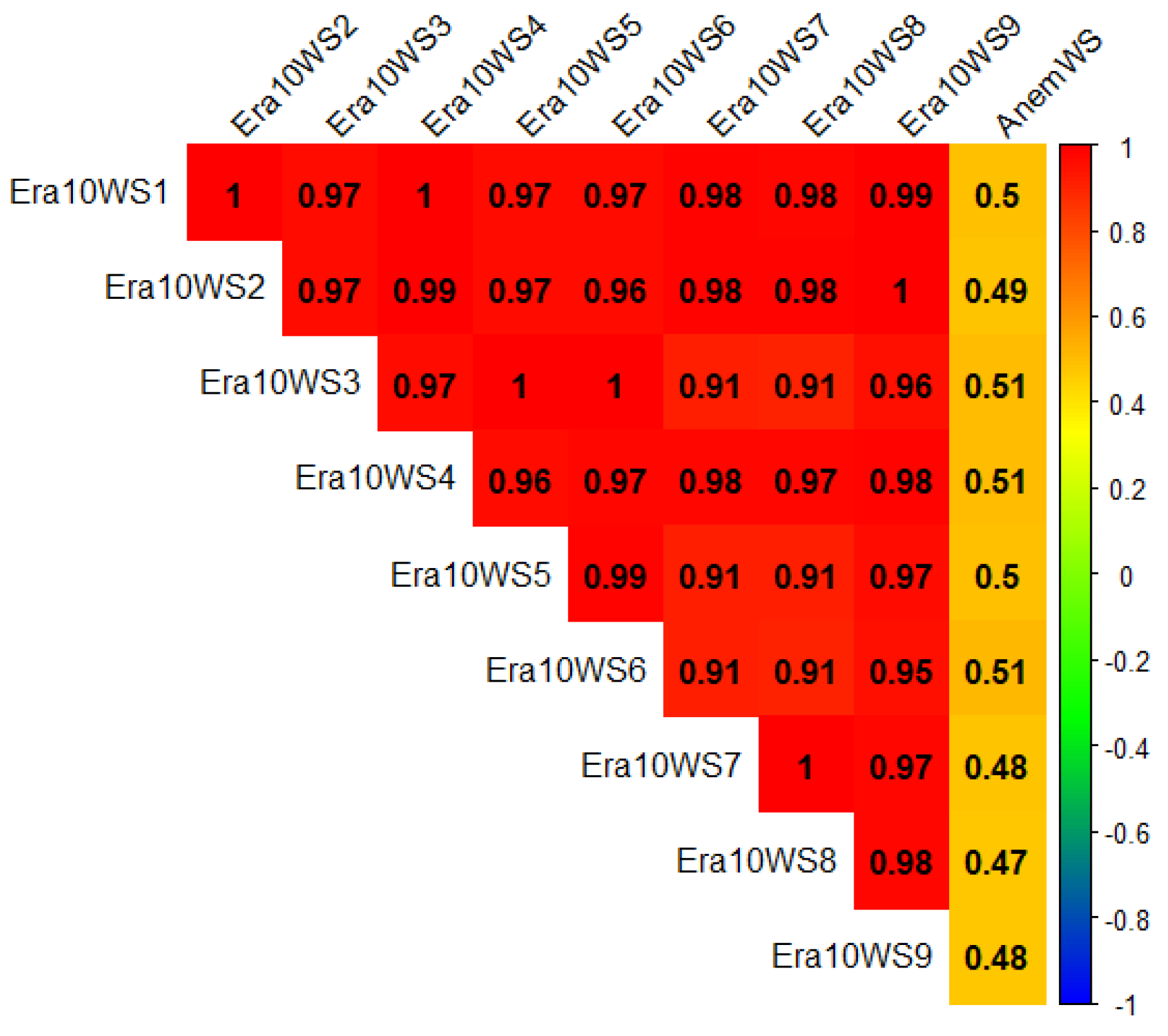
Figure 10 shows each grid point’s correlation with the rest and with the measured wind series, while Figure 11 does the same with the calibrated time series of each point. The numbering of the grid points corresponds to their proximity to the studied building, the first grid point being the closest one. It is important to note that all ERA5 grid points have a correlation of around 0.5, even the farthest ones. Considering that previous studies [35,36] have found correlations of 0.6 to be typical of buoy wind measurements against reanalysis data at open sea, this level of correlation for a much more complex terrain seems satisfactory.

Table 4. Error metrics of ERA5 grid points’ wind speeds and their calibrated counterparts against the measurements, expressed in m/s.

	ME		MAE		RMSE
	ERA5	Simple QM	ERA5	Simple QM	ERA5	Simple QM
grid point 1	1.669	0.013	1.811	0.832	2.238	1.108
grid point 2	1.663	0.013	1.811	0.842	2.243	1.121
grid point 3	1.274	0.016	1.476	0.818	1.842	1.101
grid point 4	1.642	0.013	1.781	0.827	2.202	1.101
grid point 5	1.268	0.016	1.476	0.826	1.843	1.111
grid point 6	1.274	0.013	1.473	0.814	1.84	1.093
grid point 7	2.238	0.017	2.337	0.856	2.847	1.137
grid point 8	2.215	0.018	2.319	0.864	2.832	1.151
grid point 9	1.669	0.012	1.822	0.853	2.262	1.136

shows the ME (Mean Error), MAE (Mean Absolute Error), and RMSE (Root Mean Square Error) of the uncalibrated and calibrated reanalysis’ wind speed series against the measurements for each point.

3.2. Wind Direction Prediction Results

This sections shows the results of the classification of wind direction made using RF. Figure 12 is the confusion matrix of the classification done on the testing data set, while Figure 13 is the wind rose generated using the measured wind speed and the predicted wind direction from the testing data set. It is intended to be compared with the wind rose made with the measured wind speed and direction, which can be seen in Figure 6.

3.3. Wind Speed Calibration Results

This section shows the results of the different types of calibration for only the closest grid point and using only the testing data set.

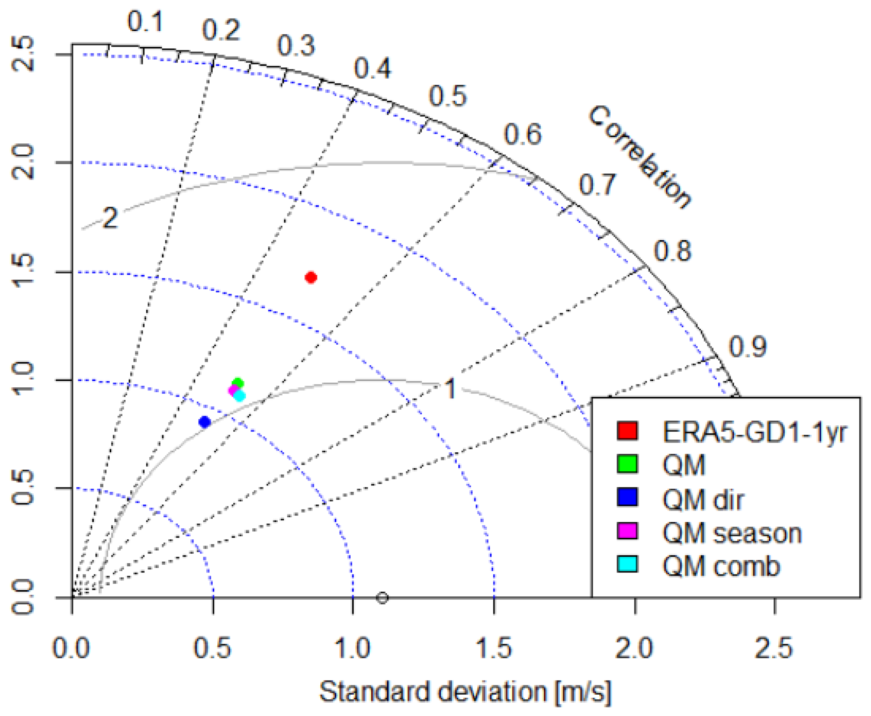
Figure 14 is the Taylor diagram that shows the correspondence of the uncalibrated wind speed time series and its various calibrated versions with the measurements.

Table 5. Error metrics of ERA5’s closest grid point’s wind speed series and its calibrations against the measurements for a 1-year period, expressed in m/s.

	ERA5-GD1-1yr	QM	QM Dir	QM Season	QM Comb
ME	1.667	0.011	−0.155	0.004	0.005
MAE	1.801	0.832	0.784	0.808	0.779
RMSE	2.235	1.1	1.033	1.073	1.046

shows the error metrics of the uncalibrated data and the calibrations against the wind measurements.

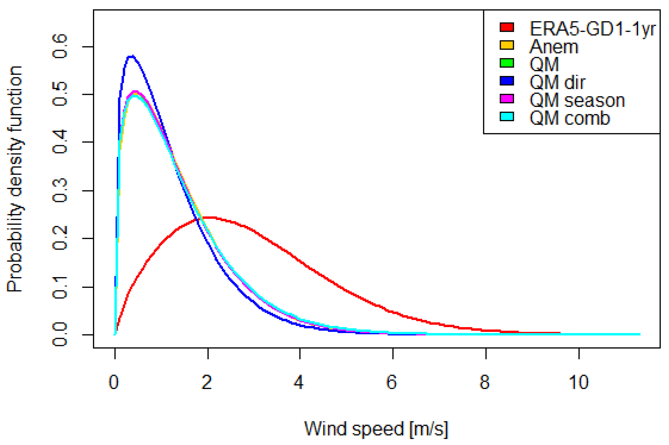
The calibrations can also be evaluated through their probability distributions. This is specially suitable for our purposes, since it is more important to get a realistic overall probability distribution from which to calculate the wind resource rather than to accurately predict wind at any given moment. In this case, the Weibull distribution was used, which is one of the types of distributions usually used in wind data analysis [30]. It was fitted for each of these wind speed times series: the measurements, the reanalysis data, and all 4 calibrations. That gave the coefficients showed in

Table 6. Coefficients of the Weibull distributions of various wind speed time series covering a 1-year period.

	ERA5-GD1-1yr	Anem	QM	QM Dir	QM Season	QM Comb
k	1.808	1.301	1.277	1.253	1.281	1.315
c	3.291	1.472	1.466	1.236	1.448	1.488

, and with those the probability density functions were plotted, as shown in Figure 15.

As the error metrics already showed, the directional calibration stands out by underestimating the wind speed. The rest of the calibrations have almost identical PDFs to that of the measured wind speed.

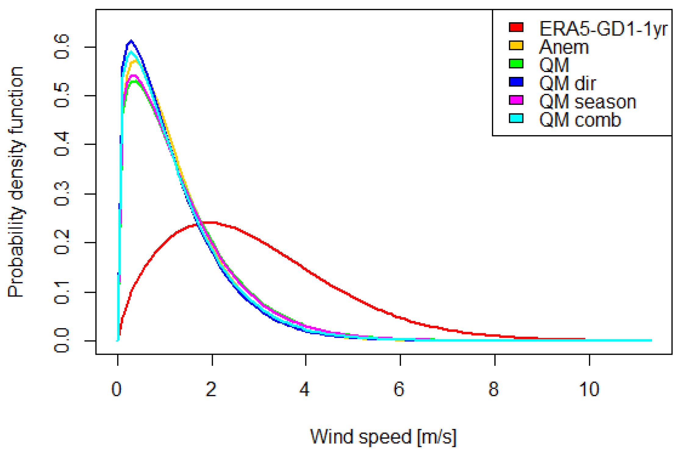
These distributions were fitted using the whole testing data set, without taking into account the measured nor the reanalysis’ wind direction. This is helpful for evaluating the calibrations themselves, but, if we want to better understand how the calibration helps estimating the production of any wind direction dependent wind turbine, we have to separately analyze the performance of the calibration using only the data points in which wind direction falls within the absorption range explained in Section 2.2.2. For that purpose, another series of Weibull distributions were fitted. In the case of the measured wind speed series, the measured wind direction was used for selecting the data points. For the calibrated series, the predicted direction was used.

Table 7. Coefficients of the Weibull distributions of various wind speed time series covering a 1-year period, using only certain wind directions.

	ERA5-GD1-1yr	Anem	QM	QM Dir	QM Season	QM Comb
k	1.728	1.232	1.203	1.194	1.209	1.236
c	3.233	1.286	1.444	1.208	1.389	1.304

shows the coefficients of these distributions, while Figure 16 shows the probability density functions.

In both Figure 15 and Figure 16, we clearly see that the measured wind speed is significantly lower than that of the reanalysis. This can be due to the different locations: the closest ERA5 grid point is located outside of the town, while the anemometer is inside the town and located at the roof of a building away from the edge, a place where CFD simulations, like that of Micallef et al. [24], indicate a low wind speed.

3.4. Energy Output Estimation Results

3.4.1. Comparison of the AEP Estimates of Each Calibration against the AEP Calculated with the Measurements

In this section, the AEP values calculated using the testing data set are used to evaluate the usefulness of the different types of calibration, alongside the predicted wind direction series. Thirty-six scenarios and 5 wind speed series are used: the measured one and the 4 types of calibration. That gives a total of AEP 180 values, shown in

Table 8. Annual Energy Production (AEP) expressed in kWh for all scenarios. The value that is closer to that of the measurements is underlined for each scenario.

Power Curve		Augmenting Factor	Wind Speed Time Series over 1 Year
Rated Power	PAGV Effect Case		Anem	QM Simple	QM Dir	QM Season	QM Comb
100 W	C1	1.28	5.51	7.55	4.5	7.22	5.98
		2.34	30.17	40.36	29.93	40.33	33.67
		3.50	69.43	89.53	71.57	87.45	74.51
	C2	1.28	12.37	17.03	11.1	16.38	13.83
		2.34	51.97	66.84	51.77	66.12	55.69
		3.50	102.54	127.98	109.5	122.59	108.57
	C3	1.28	20.23	27.04	18.85	26.73	22.58
		2.34	71.66	91.15	72.95	89.11	75.93
		3.50	130.85	155.99	137.76	148.7	134.31
150 W	C1	1.28	5.56	7.55	4.5	7.22	5.98
		2.34	33.46	45.04	31.83	44.98	37.57
		3.50	81.83	106.33	82.85	104.75	88.19
	C2	1.28	12.7	17.38	11.1	16.62	13.95
		2.34	59	77.09	58.96	77.03	64.7
		3.50	125.57	159.21	131.32	154.15	133.94
	C3	1.28	21.21	28.84	19.17	27.8	23.6
		2.34	84.26	107.85	84.08	106.3	89.52
		3.50	162.39	200.78	173.57	192.09	171.29
200 W	C1	1.28	5.56	7.55	4.5	7.22	5.98
		2.34	35.23	47.98	32.55	47.21	39.78
		3.50	89.93	118.01	91.05	117.39	99.18
	C2	1.28	13.03	17.39	11.1	16.63	13.95
		2.34	63.94	84.34	63.28	84.23	70.72
		3.50	142.99	183.14	147.03	178.89	152.96
	C3	1.28	21.56	29.49	19.19	28.23	23.92
		2.34	92.56	119.52	92.23	118.92	100.38
		3.50	188.07	236.31	198.77	227.88	199.8
250 W	C1	1.28	5.56	7.55	4.5	7.22	5.98
		2.34	36.24	49.76	32.85	48.07	40.71
		3.50	96.16	127.62	97.83	127.5	107.41
	C2	1.28	13.14	17.39	11.1	16.63	13.95
		2.34	67.55	89.72	65.69	89.72	75.12
		3.50	156.77	202.16	159.85	198.36	167.64
	C3	1.28	21.9	29.67	19.19	28.4	23.92
		2.34	99.01	129.08	98.89	128.98	108.47
		3.50	209.81	265.75	219.27	257.35	223.7

, with 36 of them corresponding to the measured data and the rest corresponding to the predictions.

To get an idea of the overall performance of each calibration across all scenarios the average relative error for each calibration was calculated. The results, in ascending order, are these: 6.77% for the directional calibration, 8.65% for the combined one, 28.20% for the seasonal one, and 31.48% for the simple calibration. In 24 out of 36 scenarios, the directional calibration’s AEP was the closest one that to that of the measured data, while, in the other 12 scenarios, the combined calibration was.

3.4.2. Estimation of Proposed Installation’s AEP and CF

Once the wind speed and direction predictions have been validated by calculating and comparing the AEP values in the testing data set, the predictive methods can be applied to the 10-year period in which the reanalysis data is available. With the results on hand, we can simulate the decision-making process we would make before deciding to install an horizontally mounted Savonious turbine on a given building. Since we still have no way to validate the accuracy of the augmenting factors described in Section 2.4.1 nor the effect of the PAGV described in Section 2.5.1, we are going to presume the intermediate cases. That means that the augmenting factor will be 2.34 and that the selected case for the PAGVs effect will be the one called C2. The calibration kind used will be the directional, not just because it has shown the best overall performance, but also because it performs best for all rated powers in this intermediate scenarios.

To perform the calibration of the 10-year reanalysis data, first, the necessary transference functions were trained using the whole 1-year period in which the measurements were taken, without cross-validating. That gives a total of 8 transference functions, one for each wind direction. Then, they were applied to the 10-year data to get a predicted wind speed time series for this period. The wind direction was predicted using the RF algorithm in a similar fashion: a single RF was trained with the 1-year data, without cross-validating and using the input parameters already explained in Section 2.4.2. Then, this RF was applied to the whole historical data.

The predicted wind speed and direction were later used to calculate 4 AEP and CF values, one for each rated power in the intermediate scenario. The results are shown in

Table 9. AEP and CF values for various wind time series and rated powers for the scenario considered as the most realistic.

Wind Series	Rated Power [W/m${}^2$]	AEP [Kwh/m${}^2$]	CF [%]
Anem over 1 year	100	51.97	5.93
	150	59	4.49
	200	63.94	3.65
	250	67.55	3.08
QM dir over 1 year	100	51.77	5.91
	150	58.96	4.49
	200	63.28	3.61
	250	65.69	3
QM dir over 10 years	100	59.59	6.8
	150	65.4	4.98
	200	68.18	3.89
	250	69.77	3.19

, which also shows the equivalent AEP and CF values calculated with the directional calibration and the measured data from the testing data set.

4. Discussion

One of the highlights of this work is the use and comparison of different kinds of QM calibrations. Twelve of them were performed with cross-validation, and all of them were successful in reducing the error between ERA5’s and the measured wind speeds. This is consistent with the previous usage of this technique in the contexts of energy potential estimation and sensor calibration.

One of the findings concerning QM is the similarity between ERA5 grid points. That can be seen in the correlations and error metrics presented in Section 3.1, which indicate that the grid points’ wind speed series do not have meaningful differences between them, and that the calibration further homogenizes them. We deduce that taking into account multiple grid points does not add meaningful information to the analysis in terms of predicting the wind speed. This is important for achieving cost-effectiveness because using a single grid point to predict the wind speed module simplifies greatly the wind resource assessment process. It also means that the current ERA5’s spatial resolution is high enough for the method presented here to be used in any building, independently of its distance to the closest grid point.

Another important finding concerning QM is the increase in the predictive capacity when training and calibrating separately different subsets of data. Seasonal categorization for QM has already been used in the field of meteorology [37]. Regarding directional categorization, one of the authors already used it for QM in the context of wave energy [14], and Applequist [38] uses it to remove bias in wind roses. However, as far as we know, this is the first time that directional categorization was used for QM in the context of wind energy, as well as the first time a combined categorization was used for wind energy estimation.

The advantage of categorized QM can be seen in the error metrics of the calibrations done on a single point without filtering by wind direction. All of them improve when compared to the uncategorized or simple QM, with just one exception: the directional calibration performs worse than the simple one in terms of the ME. Its negative value suggests that the directional calibration underestimates the wind speed. The PDFs reinforce this; they show that all calibrations get a Weibull distribution almost identical to that of the measured data, with the exception of the directional calibration, which predicts sensibly lower wind speed values. Lastly, the Taylor diagram also shows that the directional QM stands out from the rest.

When filtering by wind direction, the results are harder to interpret. First of all, the fact that the calibration’s and the measurements’ filtering are done with different wind direction series (predicted for the calibrations and measured for the measured wind speed) means that the data points used for each one are not exactly the same, so there is no way to get a Taylor diagram or error metrics. However, there is still the possibility to compare each wind series’ PDF. According to them, the seasonal and, especially, the simple calibrations overestimate the wind speed, while the combined and, especially, the directional underestimate it. However, in these cases, there does not seem to be a clear distinction between the different calibrations. It could be that the directional calibration performs worst when all wind directions are taken into account but that it performs better at the direction with the most data, which is the wind directions facing the facade. That could explain that it goes from being the worst calibration to be on par with the rest when filtering by wind direction.

Theoretically, the combined calibration should also have this advantage. It is logical to think that, since both the seasonal and the directional categorization give better results than the lack of categorization, the combined calibration would get the best results. However, that is not true because the directional calibration scores the best AEP results, and the combined one comes second. It may be that such an extensive categorization leaves insufficient data points to properly train the transference functions for the combined calibration. Since combined calibration splits the data according to 4 seasons, as well as the same directions used for the directional one, each combined QM transference function was trained with 4 times less data than the directional QM functions.

All the results already discussed seem to suggest that the directional calibration should be one of the worst at predicting the AEP. However, it is the calibration that gets closer to the AEP values calculated with the measured data in most scenarios, with the combined calibration being the one that performs best in the rest of scenarios. It is logical to think that, since both the seasonal and the directional categorization give better results than the lack of categorization, the combined calibration would get the best results. However, it may be that such an extensive categorization leaves insufficient data points to properly train the transference functions for the combined calibration. Since combined calibration splits the data according to 4 seasons, as well as the same directions used for the directional one, each combined QM transference function was trained with 4 times less data than the directional QM functions.

Regarding the use of random forest to predict wind direction, the confusion matrix shows that the classification has margin for improvement. However, the wind rose plotted using the predicted wind direction and the calculated AEP values tells us that the classification was good enough for our wind resource purposes. After all, the AEP values for the directional calibration, which depend on the predicted wind direction, have an overall relative error of 6.77%. Our interpretation of this apparent contradiction is that not every classification error has the same negative impact on the energy potential estimation. For example, there is no impact if the classification mixes two wind directions that are both inside the facade’s absorption range. Apart from that, the classification seems to mix the winds coming from both sides of the valley; that is, it tends to mix the south-western wind with the north-eastern wind. Even if this kind of error can affect the estimation, it is reasonable to think that these kinds of errors partially compensate each other’s negative impact.

Finally, a series of AEP and CF estimations were made taking into account various possible rated powers. The results show that the AEP and CF over 10 years are slightly higher than the AEP and CF calculated with both the predicted and the measured wind data. This means that the 1-year period was less windy than the typical year on that location and that, without the calibration process, the potential would have been underestimated. The AEP and CF values are also meant to help select an adequate rated power. When doing so there is a trade-off between the total amount of produced energy during the lifetime of an installation and the investment’s payback time. In this case, the low CF values tell us that a low rated power is the most reasonable choice. However, it seems that these low values come from the low measured wind speeds. Since the empirical observations made on the roof suggest that more prominent winds are usual on the edge of the selected facade, we are inclined to think that the correcting factors were not enough to compensate the inadequate location of the anemometer, as well as that more sophisticated ways to take into account the effect of the buildings geometry are needed.

5. Conclusions

In this study, different kinds of QM and a classification RF were used to predict the wind speed and direction over the roof of a building for a period of 10 years using ERA5’s data as input. These predictions were then used along different modeled power curves and different suppositions about the effect of the building’s geometry on the wind speed to come up with estimations of AEP and CF for an horizontally mounted Savonious type turbine. Even if the method was developed with the ROSEO-BIWT in mind, some aspects can also be applied to other wind turbine designs.

One of those aspects is the experiment made on the effect of the skew angle on the performance of a building integrated turbine. Apart from confirming some previous findings, like the fact that the performance of VAWTs increases with non-zero skew angle values, we also propose a way to incorporate these findings in a wind resource method. That is the absorption range, which is key to the selection of a facade and could also we used to select buildings according to their orientation. A more detailed knowledge of the effect of the skew angle could lead to more sophisticated ways to incorporate wind direction to the wind resource assessment. One of them could be modeling different power curves for different skew angles within the absorption range.

Important lessons can also be extracted from the use of QM. The fact that, when using every wind direction, even the simple calibration gets very good results in terms of PDF means that it can be used for estimating the potential energy production of wind turbines that work with every wind direction. Moving on to categorized calibrations, the success achieved by using directional and seasonal criteria seems to suggest that better results could be achieved by refining these criteria (by using more wind directions or by separating by month instead of season, for example) or by incorporating new criteria. However, the results bring up a question: why did the directional calibration perform better that the combined one even if seasonal categorization improves the results over uncategorized QM? That will have to be answered by analyzing more locations and by comparing the outcomes of different training data set sizes. For now, the best explanation is that both seasonal and directional categorization improve the calibration, but, in this study, not enough was available to properly train the combined calibration.

Apart from QM, RF was also used as a way to take into account the sensibility to wind direction. Its prediction was used to filter the wind speed predictions made via QM before implementing them on power curves. This procedure was used because QM has a great capability to match the calibrated wind speed’s PDF with that of the measurements. However, the use of RF opens up another possibility, which is using it to totally replace QM. This would be by applying regression RFs to the wind’s u and v components.

Another pending task is finding better ways to measure or estimate the concentrating effect of the wind on the edge between a facade and the roof due to the geometry of the building and its surroundings. An ideal way to validate such a method would be installing a cup anemometer directly on the edge with its rotation axis on a horizontal position, parallel to the edge, just like a horizontally-mounted Savonious would be.

References

- Council of European Union. Council Regulation (EU) No 269/2014. 2009. Available online: https://eur-lex.europa.eu/eli/dir/2009/72/oj (accessed on 1 November 2020).
- Leung, D.Y.; Yang, Y. Wind energy development and its environmental impact: A review. Renew. Sustain. Energy Rev. 2012, 16, 1031–1039. [Google Scholar] [CrossRef]
- Pedersen, E.; Waye, K.P. Wind turbine noise, annoyance and self-reported health and well-being in different living environments. Occup. Environ. Med. 2007, 64, 480–486. [Google Scholar] [CrossRef] [PubMed]
- Celik, A.N. Techno-economic analysis of autonomous PV-wind hybrid energy systems using different sizing methods. Energy Convers. Manag. 2003, 44, 1951–1968. [Google Scholar] [CrossRef]
- Chastas, P.; Theodosiou, T.; Bikas, D.; Kontoleon, K. Embodied energy and nearly zero energy buildings: A review in residential buildings. Procedia Environ. Sci. 2017, 38, 554–561. [Google Scholar] [CrossRef]
- Garcia, O.; Del Rio, M.; Ulazia, A.; Osa, J.L.; Ibarra-Berastegi, G. ROSEO: Novel Savonious-type BIWT Design Based on the Concentration of Horizontal and Vertical Circulation of Wind on the Edge of Buildings. In Proceedings of the SMARTGREENS, Heraklion, Greece, 3–5 May 2019; pp. 172–178. [Google Scholar]
- Garcia, O.; Ulazia, A.; del Rio, M.; Carreno-Madinabeitia, S.; Gonzalez-Arceo, A. An Energy Potential Estimation Methodology and Novel Prototype Design for Building-Integrated Wind Turbines. Energies 2019, 12, 2027. [Google Scholar] [CrossRef]
- Drew, D.; Barlow, J.; Cockerill, T.; Vahdati, M. The importance of accurate wind resource assessment for evaluating the economic viability of small wind turbines. Renew. Energy 2015, 77, 493–500. [Google Scholar] [CrossRef]
- Bailey, B.H.; McDonald, S.L.; Bernadett, D.W.; Markus, M.J.; Elsholz, K.V. Wind Resource Assessment Handbook: Fundamentals for Conducting a Successful Monitoring Program; Technical Report; National Renewable Energy Lab.: Golden, CO, USA; AWS Scientific, Inc.: Albany, NY, USA, 1997.
- Landberg, L.; Myllerup, L.; Rathmann, O.; Petersen, E.L.; Jørgensen, B.H.; Badger, J.; Mortensen, N.G. Wind resource estimation—An overview. Wind. Energy Int. J. Prog. Appl. Wind. Power Convers. Technol. 2003, 6, 261–271. [Google Scholar] [CrossRef]
- UPV/EHU. Escuela de Ingeniería de Gipuzkoa. Sección Eibar. Available online: https://www.ehu.eus/en/web/gipuzkoako-ingeniaritza-eskola/hasiera (accessed on 1 November 2020).
- Weekes, S.; Tomlin, A. Data efficient measure-correlate-predict approaches to wind resource assessment for small-scale wind energy. Renew. Energy 2014, 63, 162–171. [Google Scholar] [CrossRef]
- Ulazia, A.; Penalba, M.; Ibarra-Berastegui, G.; Ringwood, J.; Saénz, J. Wave energy trends over the Bay of Biscay and the consequences for wave energy converters. Energy 2017, 141, 624–634. [Google Scholar] [CrossRef]
- Ulazia, A.; Penalba, M.; Rabanal, A.; Ibarra-Berastegi, G.; Ringwood, J.; Sáenz, J. Historical Evolution of the Wave Resource and Energy Production off the Chilean Coast over the 20th Century. Energies 2018, 11, 2289. [Google Scholar] [CrossRef]
- Penalba, M.; Ulazia, A.; Ibarra-Berastegui, G.; Ringwood, J.; Sáenz, J. Wave energy resource variation off the west coast of Ireland and its impact on realistic wave energy converters’ power absorption. Appl. Energy 2018, 224, 205–219. [Google Scholar] [CrossRef]
- Fernández-Peruchena, C.M.; Polo, J.; Martín, L.; Mazorra, L. Site-adaptation of modeled solar radiation data: The SiteAdapt procedure. Remote Sens. 2020, 12, 2127. [Google Scholar]
- Polo, J.; Fernández-Peruchena, C.; Salamalikis, V.; Mazorra-Aguiar, L.; Turpin, M.; Martín-Pomares, L.; Kazantzidis, A.; Blanc, P.; Remund, J. Benchmarking on improvement and site-adaptation techniques for modeled solar radiation datasets. Sol. Energy 2020, 201, 469–479. [Google Scholar] [CrossRef]
- Costoya, X.; Rocha, A.; Carvalho, D. Using bias-correction to improve future projections of offshore wind energy resource: A case study on the Iberian Peninsula. Appl. Energy 2020, 262, 114562. [Google Scholar] [CrossRef]
- Li, D.; Feng, J.; Xu, Z.; Yin, B.; Shi, H.; Qi, J. Statistical bias correction for simulated wind speeds over CORDEX-East Asia. Earth Space Sci. 2019, 6, 200–211. [Google Scholar] [CrossRef]
- Kulkarni, S.; Deo, M.; Ghosh, S. Framework for assessment of climate change impact on offshore wind energy. Meteorol. Appl. 2018, 25, 94–104. [Google Scholar] [CrossRef]
- European Centre for Medium-Range Weather Forecasts. ERA5: Data Documentation. Available online: https://confluence.ecmwf.int/display/CKB/ERA5%3A+data+documentation (accessed on 8 October 2020).
- Choi, C.K.; Kwon, D.K. Wind tunnel blockage effects on aerodynamic behavior of bluff body. Wind Struct. Int. J. 1998, 1, 351–364. [Google Scholar] [CrossRef]
- Chowdhury, A.M.; Akimoto, H.; Hara, Y. Comparative CFD analysis of vertical axis wind turbine in upright and tilted configuration. Renew. Energy 2016, 85, 327–337. [Google Scholar] [CrossRef]
- Micallef, D.; Van Bussel, G. A Review of Urban Wind Energy Research: Aerodynamics and Other Challenges. Energies 2018, 11, 2204. [Google Scholar] [CrossRef]
- Simão Ferreira, C.J.; Van Bussel, G.J.; Van Kuik, G.A. Wind tunnel hotwire measurements, flow visualization and thrust measurement of a VAWT in skew. J. Sol. Energy Eng. 2006, 128, 487–497. [Google Scholar] [CrossRef]
- Mertens, S. Wind Energy in the Built Environment: Concentrator Effects of Buildings; Multiscience Publishing: Brentwood, UK, 2006; Volume 30. [Google Scholar]
- Ulazia, A.; Penalba, M.; Ibarra-Berastegui, G.; Ringwood, J.; Sáenz, J. Reduction of the capture width of wave energy converters due to long-term seasonal wave energy trends. Renew. Sustain. Energy Rev. 2019, 113, 109267. [Google Scholar] [CrossRef]
- Svetnik, V.; Liaw, A.; Tong, C.; Culberson, J.C.; Sheridan, R.P.; Feuston, B.P. Random forest: a classification and regression tool for compound classification and QSAR modeling. J. Chem. Inf. Comput. Sci. 2003, 43, 1947–1958. [Google Scholar] [CrossRef] [PubMed]
- Chen, C.; Liaw, A.; Breiman, L. Using random forest to learn imbalanced data. Univ. Calif. Berkeley 2004, 110, 24. [Google Scholar]
- Manwell, J.F.; McGowan, J.G.; Rogers, A.L. Wind Energy Explained: Theory, Design and Application; John Wiley & Sons: Hoboken, NJ, USA, 2010. [Google Scholar]
- Polman, A.; Knight, M.; Garnett, E.C.; Ehrler, B.; Sinke, W.C. Photovoltaic materials: Present efficiencies and future challenges. Science 2016, 352, aad4424. [Google Scholar] [CrossRef] [PubMed]
- MAXON MOTOR. Available online: https://www.maxonmotor.com (accessed on 1 November 2020).
- Mohamed, M.; Janiga, G.; Pap, E.; Thévenin, D. Optimization of Savonius turbines using an obstacle shielding the returning blade. Renew. Energy 2010, 35, 2618–2626. [Google Scholar] [CrossRef]
- Altan, B.D.; Atılgan, M. A study on increasing the performance of Savonius wind rotors. J. Mech. Sci. Technol. 2012, 26, 1493–1499. [Google Scholar] [CrossRef]
- Ulazia, A.; Saenz, J.; Ibarra-Berastegui, G. Sensitivity to the use of 3DVAR data assimilation in a mesoscale model for estimating offshore wind energy potential. A case study of the Iberian northern coastline. Appl. Energy 2016, 180, 617–627. [Google Scholar] [CrossRef]
- Ulazia, A.; Sáenz, J.; Ibarra-Berastegui, G.; González-Rojí, S.J.; Carreno-Madinabeitia, S. Using 3DVAR data assimilation to measure offshore wind energy potential at different turbine heights in the West Mediterranean. Appl. Energy 2017, 208, 1232–1245. [Google Scholar] [CrossRef]
- Rojas, R.; Feyen, L.; Dosio, A.; Bavera, D. Improving pan-European hydrological simulation of extreme events through statistical bias correction of RCM-driven climate simulations. Hydrol. Earth Syst. Sci. 2011, 15, 2599–2620. [Google Scholar] [CrossRef]
- Applequist, S. Wind Rose Bias Correction. J. Appl. Meteorol. Climatol. 2012, 51, 1305–1309. [Google Scholar] [CrossRef]
- R Core Team. R: A Language and Environment for Statistical Computing; R Foundation for Statistical Computing: Vienna, Austria, 2017. [Google Scholar]
- Gudmundsson, L.; Bremnes, J.B.; Haugen, J.E.; Engen-Skaugen, T. Technical Note: Downscaling RCM precipitation to the station scale using statistical transformations—A comparison of methods. Hydrol. Earth Syst. Sci. 2012, 16, 3383–3390. [Google Scholar] [CrossRef]
- Liaw, A.; Wiener, M. Classification and Regression by randomForest. R News 2002, 2, 18–22. [Google Scholar]
Figure 1.
Diagram that summarizes the methodology and data used.
Figure 2.
Location of the studied building (red) and ERA5 grid points (blue). The grid points are numbered according to their proximity to the anemometer.
Figure 3.
Design and dimensions of the small Savonius model and the PAGVs (Power Augmenting Guiding Vanes) (a)–(c) and the corresponding photos of the small-scale building with the real Savonius and the PAVs (d)–(f).
Figure 4.
Scheme of the skew angle for our small scale experiment and the horizontal axis turbine with the incoming wind field (vectors above) in the wind tunnel. 0 corresponds to wind direction perpendicular to the facade.
Figure 5.
Boxplots of rotational speed of the small-scale longitudinal turbine at different wind speeds and skew angles.
Figure 6.
Wind rose of the wind measured in the building.
Figure 7.
Representation of the studied building and the relevant information to choose a facade for the installation. The wind rose is the same of
Figure 6. The light blue area corresponds to the absorption range of the selected facade. The dotted red line marks the valley’s direction. The green square marks the anemometer’s location on the roof.
Figure 8.
Frequency of each measured wind direction during the studied 1-year period.
Figure 9.
Estimated power curve of the Savonious drag-type turbine for a 250 W generator without guiding vanes or plates.
Figure 10.
Correlation table of the wind speed series from each ERA5 grid point and the measured wind speed series.
Figure 11.
Correlation table of the calibrated wind speed series from each ERA5 grid point and the measured wind speed series.
Figure 12.
Confusion matrix of the results of the wind direction classification performed on the testing data set using random forest (RF).
Figure 13.
Wind rose that combines the measured wind speed with the predicted wind direction from the testing data set.
Figure 14.
Taylor diagram of the various calibrations and the uncalibrated wind speed time series from the closest grid point against the measurements.
Figure 15.
Probability density functions of the Weibull distributions of various wind speed series covering a 1-year period.
Figure 16.
Probability density functions of the Weibull distributions of various wind speed series covering a 1-year period, using only certain wind directions.