Solving Order Planning Problem Using a Heuristic Approach: The Case in a Building Material Distributor

Abstract

For building material distributors, order planning is a key process as a result of the increase in construction projects’ scale and complexity. In this paper, the integration of simulation modeling and the response surface methodology (RSM) is presented to solve an order planning problem in the construction supply chain. The interactions of various factors are examined to observe their effects on key system measurements, and a combination of factor levels is determined to achieve the optimal performance. RSM is applied to find the possible values of the optimal setting for system responses, which consists of three main steps: central composite design (CCD), Box–Behnken design (BBD), and a comparison of both designs. The model is tested with a realistic case study of a building material distributor in Vietnam to demonstrate its effectiveness. Controllable factors (independent variables), which are the review period (T), order quantity (Q), and safety stock (SS), are found to significantly affect system responses, which are the total cost (TC) and customer service level (CSL). The results provide the best settings of factor levels that produce the possible minimum TC and maximum CSL. The developed framework could be applied as a useful reference for decision-makers, purchasing managers, and warehouse managers to obtain the most suitable order policy for a robust order planning process.

1. Introduction

Buildings are becoming increasingly complex because of the ongoing rise in the size and scope of construction projects. Following that, the rising segmentation of the construction industry goes hand-in-hand with the growth of specialist suppliers or contractors, and the diversity of products, designs, and control activities [1]. Relationships in the construction industry are short-term and normally informal/ad-hoc, which focus on the projects, not the business. Construction demand is inherently unstable as the industry is project-based with defined start and endpoints, and a conventional separation between design and construction. Demand is viewed by temporary coalitions as a series of competitively tendered prototypes. Competencies between construction projects vary from time to time and are distinguished from each other. In the supply chain of the construction industry, order planning is the key process, especially for building material distributors. Adequate order planning is quintessential to a more comprehensive integrated supply chain solution, by which businesses can achieve real-time capabilities to act as an intermediary between manufacturing, sales, and customer service concerns, in order to guarantee on-time, effective and reliable processes of order fulfillment and delivery [2]. For building material distributors, the most common problems are inaccurate forecasts of annual projects received and the overloading in stock due to the delayed construction work progress. Therefore, demand forecasting and inventory management are crucial tasks in the order planning process, as the progress of construction projects is often not always as smooth as scheduled. Accurately forecasting spikes in demand and appropriate levels of safety stock can give a competitive advantage in the industry.

In the context of demand variability, sufficient order planning policies are crucial [3]. Some common challenges of order planning problems in all different types of industries are accurate monitoring of all stock-keeping units (SKUs) and stock levels, availability of historic sales forecasting data, calculating correct supplier lead-times, new product introductions, and centralizing stock control [4]. In this context, building material distributors often deal with serious stock-outs (unknown/unaware projects) or extreme overstock (delayed projects). Consequently, additional costs are incurred due to extra shipments, transportation and transferring activities, inventory holding, and handling costs, to name a few. In addition, the expectation of customers for timely and reliable products and service is ever-increasing, so that a more efficient ordering operation is indispensable and is a key measure for customer service. Incomplete and delayed orders are the most common causes of worsening customer satisfaction. Hence, strategies in ordering planning problems, namely which order to fulfill and in what sequence that strongly affects customer satisfaction and businesses’ profits, as it decides how to divide the inventory between orders and how to attend to orders to provide an efficient process [5].

Some strategies are used to mitigate risk in the ordering process: classifying stock [6], drop-shipping [3], prepurchasing stocks [7], using hybrid strategies [8,9], and setting stock minimization policies [10]. Many studies developed stock control policies to solve the problem of managing inventory. They applied lot sizing, stockpiling, and period length instead of controlling on-hand inventory, at the same time examining certain stochastic variables in the ability to respond with high demand fluctuations and shortages in the multistage supply chain [11,12]. In practice, demands vary from time to time, they are more of fuzzy numbers than deterministic ones. Problems concerning production and inventory decisions are regarded as a joint economic lot-sizing problem (JELP), of which a vendor and a buyer with stochastic demand and variable lead time are considered [13]. Jauhari and Laksono [14] solved the JELP with the demand changing over time, imperfect production emission cost, and defective production rate. By considering the fuzzy annual demand, their mathematical model contributed to the existing inventory literature. Chiang Kao and Wen-Kai Hsu [15] provided a framework for the development of the fuzzy total inventory cost with uncertain demand and the used Yager’s ranking method to minimize the total cost and to prevent lost-sales. Kim et al. [16] introduced a multiperiod newsvendor problem, which formulated integer recourse decisions as a multistage stochastic programming model. The proposed method offered novel knowledge to optimize the trade-off between delivery, transshipment, shortage, and holding costs, which is the gap to other studies that suggested stochastic inventory models. Additionally, most studies suggested different considerations for customer service’s perception, assumed that quality products, sales price, corporate social responsibility, and recycling commitment are key factors to the customer service level [17,18,19,20,21,22].

In this paper, simulation modeling is developed to explain the ordering process for building materials in a distributor. For this case study, key system performance measures are the total cost (TC) and the customer service level (CSL). The total cost includes transportation cost, holding cost, over-storage cost, and shortage cost. On the other hand, CSL simplifies by the accumulation of total demand satisfied. Parameters of products include unit weight, unit holding cost, unit shortage cost, and unit over-storage cost. Controllable factors of the ordering process are the monthly demand, review period (T), order quantity (Q), and safety stock (SS), which are treated as independent variables. Using RSM, the best settings, which are appropriate combinations of T, Q, and SS are determined as an indicator to measure the performance of each possible setting, in which TC and CSL are response variables. The solution is to place the right order quantities at the right time, with the appropriate safety stock to achieve customer satisfaction levels between 90 and 95 percent at minimum costs.

The contributions of our paper are three-fold. First, the paper proposed a computational framework to solve the order planning problem by a heuristics approach using RSM, which includes the central composite design (CCD), Box–Behnken design (BBD), and variance dispersion graph (VDG), in order to offer the best possible time-efficient and resource-saving solution in terms of key performances. Most exact methods cannot solve the problem within a satisfactory amount of time, especially for large-scale problems. In contrast, most heuristics allows decision-makers to obtain a feasible and timelier solution. For order planning problems in the construction industry, managing the demand, duration, and progress between projects that are supposed to be implemented simultaneously by a distributor is a complicated task. Thus, to facilitate the practical process and available resources, heuristics can provide decision-makers feasible short-term solutions within a reasonable amount of time. Second, the proposed heuristic model is validated by a realistic case study of a distributor in Vietnam to illustrate the effectiveness of the model’s result. Third, the managerial implications of the paper could be a beneficial guide for decision-makers, purchasing managers, and warehouse managers to obtain the most suitable order policy for a robust order planning process. In addition, the practical contribution of this study is the comprehensive insight into order planning problems contributed by the case study of the building material distributor in Vietnam.

The paper is divided into five sections. The introduction and relevant studies are discussed in the first section. In the second section, the research procedure and related methodology are included. This paper proposed a computational framework to solve the order planning problem. Additionally, the case study of a distributor is presented in the third section. In the fourth section, the empirical results are shown, including the results of excel spreadsheet simulation, and experimental design of central composite design, and Box–Behnken design. Moreover, discussions, conclusions, and recommendations are given in the last section.

2. Literature Review

This paper combined simulation modeling and the response surface methodology (RSM) to solve an order planning problem. A simulation and/or computational experiment are used to model a comprehensive supply chain network that corresponds with a number of supply chain operational elements and management levels [23]. Some studies that proposed simulation-based optimization models to explain supply chain systems are discussed in [24,25]. Supply chain dynamics (response) are typically quantified in terms of order and inventory variance ratios. To experiment with the stochastic supply chain model, a simulation modeling approach was adopted. As a result of modifying the controllable variables, the simulation model was run to generate the various supply chain responses, and thus the functional relationship could be fitted and its response surface defined. RSM is a feasible alternative to modeling, on the other hand, which optimizes stochastic, dynamic, and complex systems such as supply chains. This approach is used to find a functional link between the complex responses of the supply chain and significant controllable variables that influence them [26]. Giddings et al. [27] used RSM for optimality analysis of the cost coefficients in mixed integer linear programming in facility location problems. The study implemented the design of experiments and applied least squares regression to determine cost coefficients that significantly affect the optimal total cost surface within setup coefficient ranges. In a problem of finding the suitable capacity for a factory, Shang et al. [28] aimed at integrating simulation, Taguchi techniques, and RSM. Findings of this hybrid approach is a useful reference for businesses to analyze the dynamic relations among various factors, so as to determine the best combination of their levels that optimizes the impact of demand uncertainty on the performance of the supply chain. Buchholz et al. [29] developed a hybrid model of a process-based simulation ProC/B toolset and RSM for the optimization of the process chain models. In this paper, the experiment of the central composite design was applied to find the optimal values of response variables. The “bullwhip” effect, known also as order variance amplification, is a major cause of supply chain deficiencies. Hassanzadeh et al. [30] studied a three-stage simulation with a single retailer, a single wholesaler, and a singer-producer under both centralized and decentralized chains, in order to analyze the causes of the bullwhip effect from two dimensions of order and inventory variance using RSM. As an extension, a multiobjective minimization problem in which the order and inventory variance ratios are separated into two objective functions was developed by Devika et al. [31]. RSM was used in a hybrid evolutionary approach to analyze interactions between the variance ratios and their corresponding effects, in order to optimize supply chain systems. For measuring design parameters on the bullwhip effect and dynamic responses, Tang et al. [32] analyzed its influences on the supply chain’s performance using a hybrid Taguchi and dual RSM. This paper offered practical solutions to the supply chain managers and designers in the trade-off between customer service level and inventory holding cost under an uncertain environment.

To provide an overview of recent contributions, several studies that presented relevant problem characteristics are shown in

Table 1. List of common problem characteristics for several previous studies.

Authors	Independent Variables	Response Variables	Methods/Techniques
Zhang et al. [33], 2015	Number of orders Planning horizon Production capacity	Penalty for delivery Penalty for order Inventory cost Production cost	NLP PSO algorithm
Guo et al. [34], 2015	Due date of order Production workload Capacity efficiency	Completion time Production capacity Processing time	MOLP DOE
Lim et al. [35], 2017	Demand variability Lead time	Holding cost Supply cost Safety stock	Simulation modeling MOLP
Singha et al. [36], 2017	Reorder point Order quantity Inventory policies	Ordering cost Shortage cost Holding cost Over-ordering cost	EOQ (R, Q) model Mathematical model
Jansen et al. [37], 2019	Planned lead time Production plan	Holding cost Penalty cost	Mathematical model
Thinakaran et al. [40], 2019	Time-varying Stock demand Lot size	Backorder Lost sales	EOQ EPQ
Wang et al. [42], 2020	Ordering quantity Reorder point Target stock Inventory policies	Holding cost Penalty cost	Simulation modeling DOE
Kokuryo et al. [38], 2020	Order quantity Production schedule Order period	Delivery time Profit	Mathematical model
Tai et al. [39], 2020	Order quantity Lead time Inventory policies	Over-storage amount Inventory cost	EOQ (S, T) model Mathematical model
This paper, 2020	Review period Order quantity Safety stock	Holding cost Shortage cost Over-storage cost Transportation cost	Simulation modeling RSM

Note: NLP: nonlinear programming, PSO: particle swarm optimization, MOLP: multi-objective linear programming, DOE: design of experiment, EOQ: economic order quantity, EPQ: economic production quantity, RSM: response surface methodology.

. Concerning order planning problems, many studies approached exact methods such as NLP [33], MOLP [34,35], and mathematical models [36,37,38,39]. The widely used method is applying inventory policies such as the economic order quantity (EOQ), economic production quantity (EPQ), (S, T), or (R, Q) model [36,39,40]. The order planning problem is actually the flow shop (FS) problem, which is an NP-hard problem [41]. Most exact methods cannot solve large-scale problems within an acceptable amount of time. Therefore, heuristics [33,42] have widely been applied currently, which produce good feasible solutions timely and effectively. In this paper, to optimize an order planning problem, namely to minimize total relevant costs and maximize customer satisfaction level, RSM was used to determine the best combination of the system parameters. Independent variables, which are the review period (T), order quantity (Q), and safety stock (SS), were treated as factors for response variables, which are the total cost (TC) and customer service level (CSL). Analytical approaches have many limitations to simultaneously solve two or three factors [23]. It is difficult to observe the factor interactions and predict their effects on the overall objective when multiple factors are considered at a time. By using RSM, our research aims to determine the best parameter settings of considered factors to find the possible optimum values of the responses. Findings are expected to offer purchasing managers or decision-makers to obtain the optimal combination of the levels of independent factors, which strongly affect the key system performance measures, i.e., total relevant costs and customer satisfaction level.

3. Materials and Methods

3.1. Response Surface Methodology (RSM)

Response surface methodology (RSM) was used to design and perform an experimental design via statistical and mathematical approaches. RSM was applied to determine the possible optimal values of factors (i.e., independent variables) to minimize and/or maximize the outputs (response variables). RSM was assumed that there is no correlation among independent variables. There are many stages to perform the process of optimization using RSM. The following parts present the simple and polynomial regression model [43,44,45,46].

The simple regression model is presented in Equation (1) as follows.

$$Y={\beta }_o+{\beta }_1{X}_1+{\beta }_2{X}_2+\dots +{\beta }_k{X}_k+\epsilon$$

(1)

where Y denotes response variables, $X_1,X_2,\dots X_k$ denotes independent variables, k is the total of independent variables, ${\beta }_o$ is the intercept, ${\beta }_1,{\beta }_2,\dots {\beta }_k$ is the slope, and $\epsilon$ is the random error.

Equation (2) shows the quadratic polynomial regression model.

$$Y={\beta }_o+{\displaystyle \sum }{\beta }_1{X}_1+{\displaystyle \sum }{\beta }_2{X}_2{}^2+{\displaystyle \sum }{\beta }_3{X}_1{X}_2+\dots +\epsilon$$

(2)

where Y denotes response variables, $X$ denotes independent variables, ${\beta }_o$ is the intercept, ${\beta }_1$ is the coefficient for the linear terms, ${\beta }_2$ is the coefficient for the square terms, ${\beta }_3$ is the coefficient for the interaction among terms, and $\epsilon$ is the random error.

In the polynomial regression model, CCD and BBD are two types of experimental designs often referred to by the researchers. CCD is an experimental design with two-level. Minitab provides the rotatability value (α) to ensure the design displays the desirable properties. Meanwhile, BBD is the experiment with a three-level design. BBD does not have the rotatability value (α) and embedded factorial design. Points on the diagrams represent the experimental runs of CCD and BBD are shown in Figure 1 as follows [47].

3.2. A Computational Framework

In this paper, a computational framework was built (Figure 2), which consists of two parts, described as follows: (1) an Excel spreadsheet was used to develop the order planning model, and calculate the response variables, i.e., total cost and customer service level. Then, (2) Minitab was used to find the feasible values of the optimal setting for those responses using RSM, CCD, and BBD. Besides, a VDG was applied to validate these experimental designs. Three independent variables were being considered to have effects on the response variables in this experiment, consisting of the review period (T, month), order quantity (Q, unit), and safety stock (SS, unit). The combination in the total cost (TC, USD) that includes the holding cost, shortage cost, over-storage cost, transportation cost, and customer service level (CSL, %) were chosen as response variables of the order planning model.

4. A Case Study

4.1. Problem Description

The description of the primary building materials of a distributor in Vietnam is shown in Figure 3. There are four main material products for coating in construction works: Spectite CW100 (a), Spectite WS (b), Spectite HP600 (c), and Speccoat PE145 (d). The statistical summary of historical sale data (2017–2019), and the component costs of materials are demonstrated in

Table 2. Statistical summary of historical sale data added up to 36 months (2017–2019).

2017	Spectite CW100	Spectite WS	Spectite HP600	Speccoat PE145
Max	1663	131	224	40
Min	215	0	0	1
Avg	1044.58	45	36.33	5.83
SD	470.18	47.13	63.58	11.81
2018	Spectite CW100	Spectite WS	Spectite HP600	Speccoat PE145
Max	2140	965	100	114
Min	411	0	0	2
Avg	1093.50	198.17	21.42	31.83
SD	538.73	265.93	35.64	34.91
2019	Spectite CW100	Spectite WS	Spectite HP600	Speccoat PE145
Max	2290	359	75	83
Min	219	0	0	0
Avg	1387.75	142.42	32.67	30.17
SD	649.19	124.85	30.79	24.88

Note: calculated by the researchers.

and

Table 3. Component costs of materials.

Materials	Spectite CW100	Spectite WS	Spectite HP600	Speccoat PE145	Unit
Packing size	22 kg/set	25 kg/bag	20 L/pail	15 L/pail	-
Wholesale price	11	20	78	49.5	USD/unit
Receipt cost	12.93	22.12	84.73	54.70	USD/unit
Selling price	18.42	32.89	116.22	87.72	USD/unit
Holding cost	0.075	0.129	0.494	0.319	USD/unit/month
Shortage cost	0.553	0.987	3.487	2.632	USD/unit
Over-storage cost	0.162	0.277	1.059	0.684	USD/unit/month

Note: calculated by the researchers.

, respectively.

Currently, the company places orders from a supplier every three or four months. Afterward, the transportation freight charge for 20 ft and 40 ft containers that are used for shipments directly to a warehouse. For inventory management, each unit of products (set, pail, or bag) is charged for holding cost per unit per month. Over-storage cost per unit is charged when ending inventory excesses the warehouse capacity. Shortage cost per unit is charged if satisfied demand is less than the actual demand. Key performances are measure periodically, which are the total cost, calculated by the sum of holding inventory, shortage cost, over-storage cost, and transportation cost, as presented in Equation (3); and the customer service level, which is determined by the accumulation of the total demand satisfied, as shown in Equation (4). Subsequently, the company is facing a problem in which should setup different factors (i.e., referred to independent variables in this paper) that affect the performance of the inventory system. Therefore, designing a computational framework to find the feasible values of the optimal setting of levels for independent variables that strongly affect the minimum total cost of holding cost, shortage cost, over-storage cost, transportation cost, and customer service level is needed.

Total cost (TC) can be calculated from the following Equation (3):

$$TC=C_h+C_s+C_o+C_t$$

(3)

where $C_h$ is holding cost, $C_s$ is shortage cost, $C_o$ is over-storage cost, and $C_t$ is transportation costs.

The customer service level (CSL) in this model simplifies by the accumulation of the total demand satisfied, and it can be calculated from the following Equation (4):

$$CSL=\frac{Demand-ShortageAmount}{TotalDemand}\times 100\%$$

(4)

4.2. Numerical Example

In order to demonstrate the model’s effectiveness, the authors chose “Spectite CW100”, the key product of the company. Compared to other products, Spectite CW100 is always indispensable for construction projects, yet often running out of stock. Additionally, this product was selected based on ABC analysis (i.e., highest sale volume and high order frequency) [48,49]. The ABC classification divides inventory stock-keeping units (SKUs) into three groups based on their annual monetary purchases. These SKUs are high-value items, i.e., the 15–20% of the total inventory that accounts for 75–80% of the total annual inventory value. The product is distributed to customers and given inventory carrying cost, shortage cost, and over-storage cost of each unit. Based on product behaviors and the current order planning process, the interval ranges of the variables were set by the decision-makers as shown in

Table 4. The interval ranges of the variables.

No.	Variables	Notation	Interval Range	Unit
1	Review period (categorical factor)	T	(3, 4)	Month
2	Order quantity (continuous factor)	Q	(3500, 4000)	Unit
3	Safety stock (continuous factor)	SS	(1000, 1300)	Unit
4	Total cost (response)	TC	TC (Ch, Cs, Co, Ct)	USD
5	Customer service level (response)	CSL	CSL (90% and 95%)	%

Note: calculated by the researchers.

and were chosen as potential values in the factorial design for this problem.

5. Empirical Results

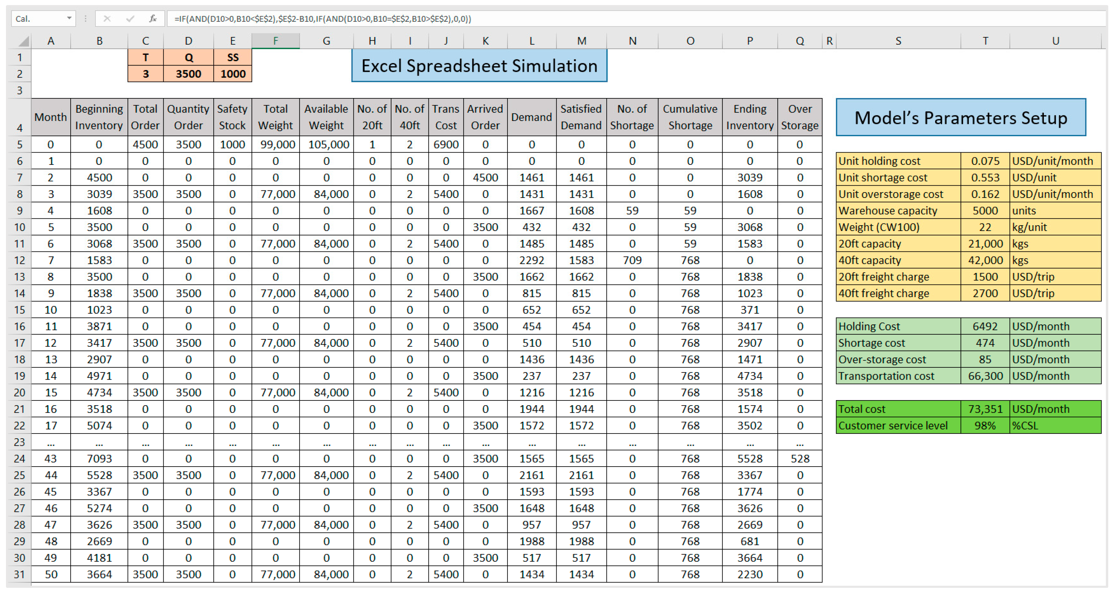
5.1. Excel Spreadsheet Simulation

First, the authors pivoted the quantity of historical sale data to count monthly order frequency to generate the probability of demand. Next, the authors used the random function in excel to simulate customer demand and get the values response variables (TC and CSL). The experimental design was created using a central composite design and Box–Behnken design to find the possible independent variables settings for solving the order planning problem. The excel spreadsheet simulation template for the experimental design is described in Figure 4.

In this paper, a case study of a distributor is presented to demonstrate the effectiveness of the developed computational framework to solve the current order planning problem in the company.

The model’s parameters setup is described as follows.

• Unit holding cost, C_h = 0.075 USD/unit/month;
• Unit shortage cost, C_s = 0.553 USD/unit;
• Unit over-storage cost, C_o = 0.162 USD/unit/month;
• Warehouse capacity = 5000 units;
• Weight (CW100) = 22 kg/unit;
• Maximum capacity of container type 20 ft = 21,000 kg;
• Maximum capacity of container type 40 ft = 42,000 kg;
• Freight charge of container type 2 0ft = 1500 USD/trip;
• Freight charge of container type 40 ft = 2700 USD/trip.

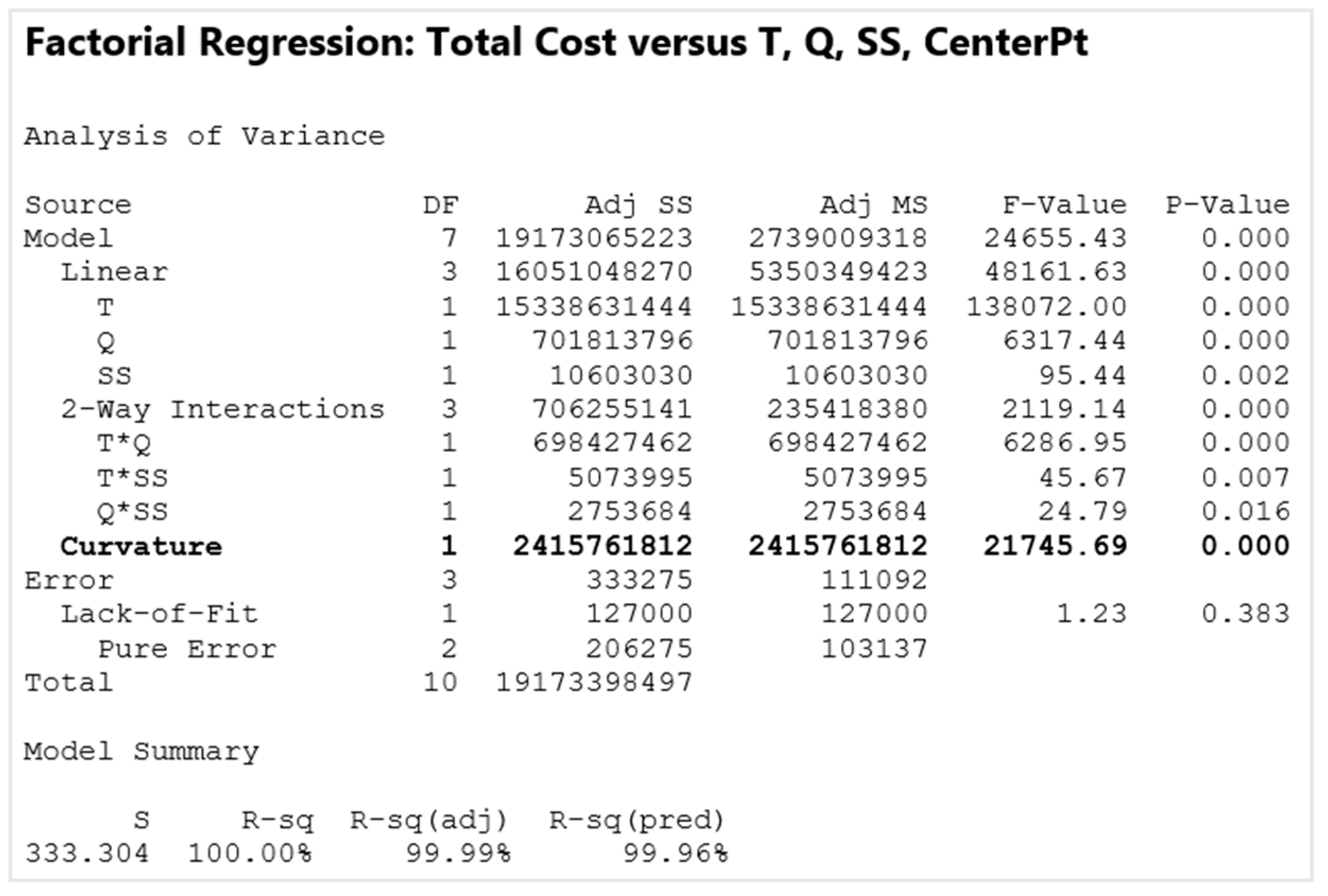
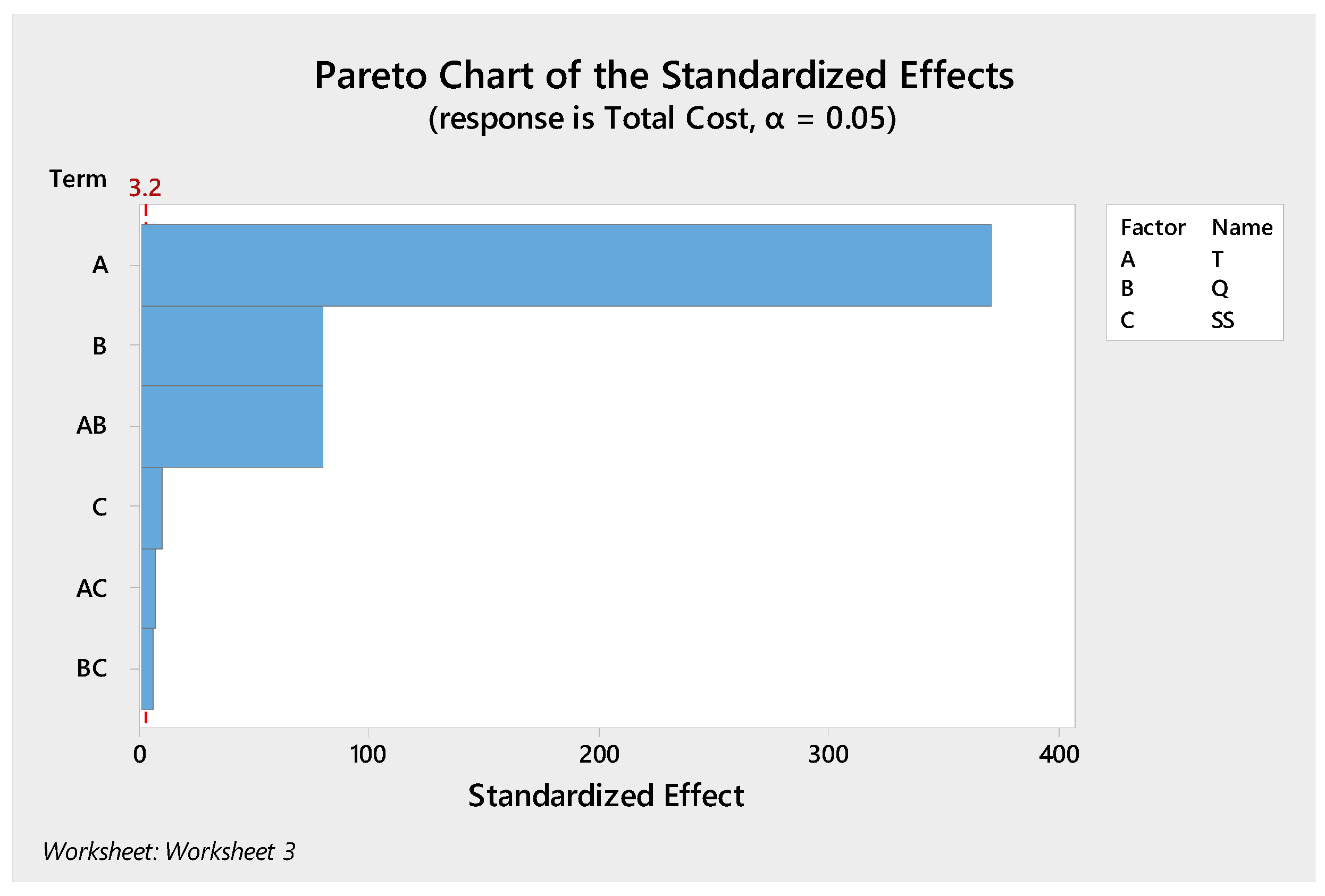
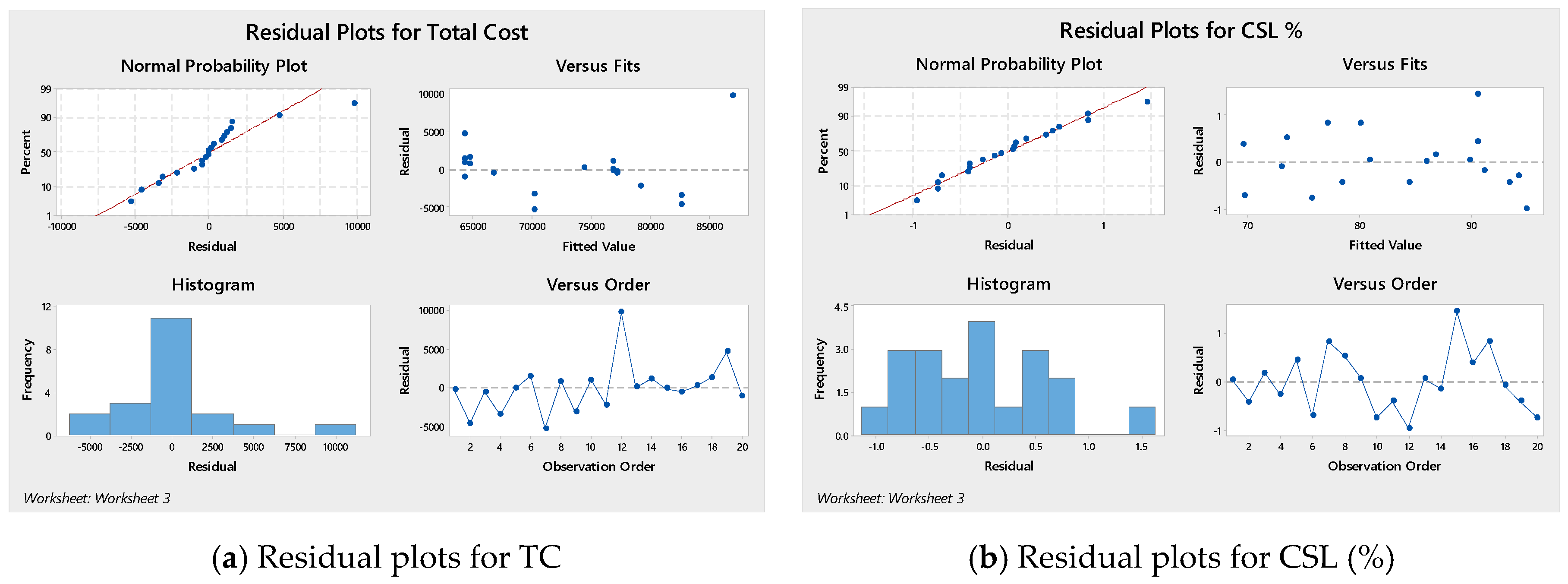
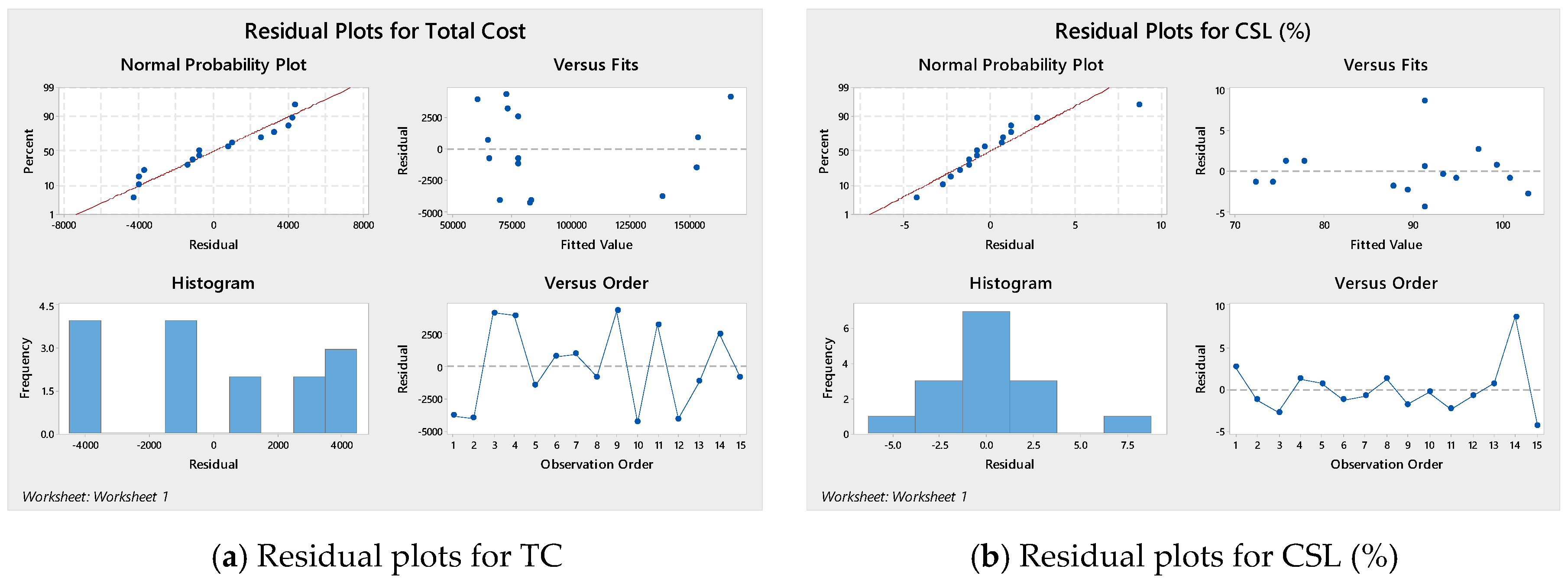
5.2. Statistical Analysis

In the initial step, the statistical analysis using the full factorial design was performed to test the curvature of the response variables (TC and CSL) and independent variables (T, Q, and SS). Then, the data was analyzed in Minitab using stepwise, and the result shows curvature. The analysis of variance of factorial regression and the Pareto chart of the standardized effects are presented in Figure 5 and Figure 6, respectively.

In Figure 5, the analysis of variance of factorial regression, the results suggested that the model had significant curvature because the p-value (p-value = 0.000) was less than the confidence level at 95%. The presence of curvature usually indicates that the factor settings were near a feasible response value. Therefore, two response surface designs, central composite design, and Box–Behnken design were considered afterward to find the possible parameter settings for this case. In the step of full factorial design, for the starting center point, T = 3, Q = 3500, and SS = 1000, were considered. Figure 6 shows the Pareto chart of the standardized effects from the results and factors. It can be seen that their interaction significantly affected the model’s results.

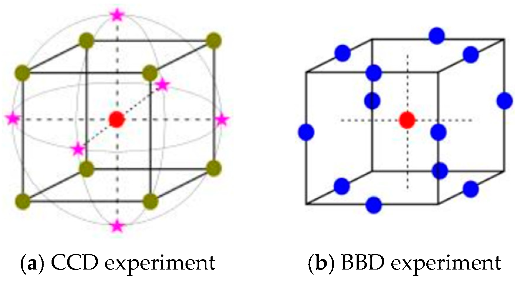
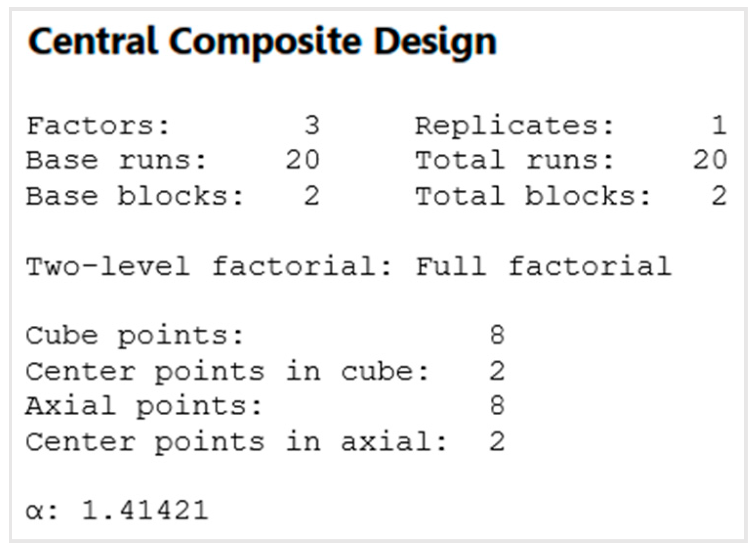
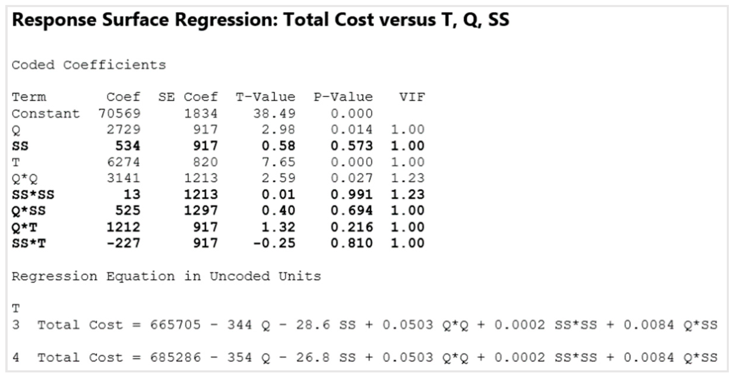
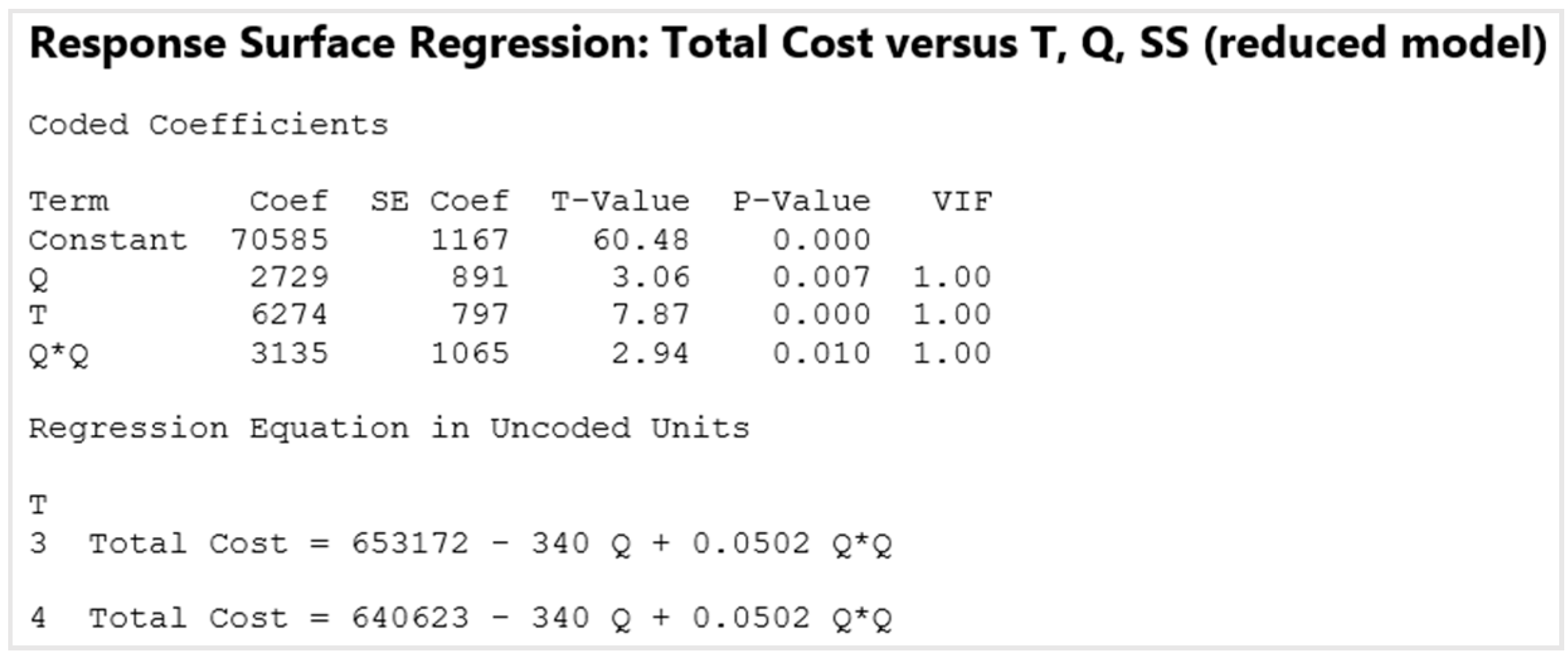
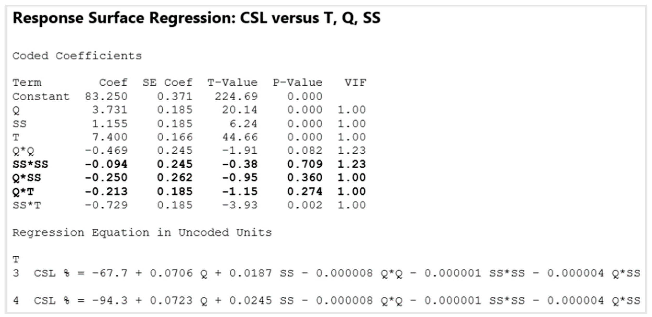
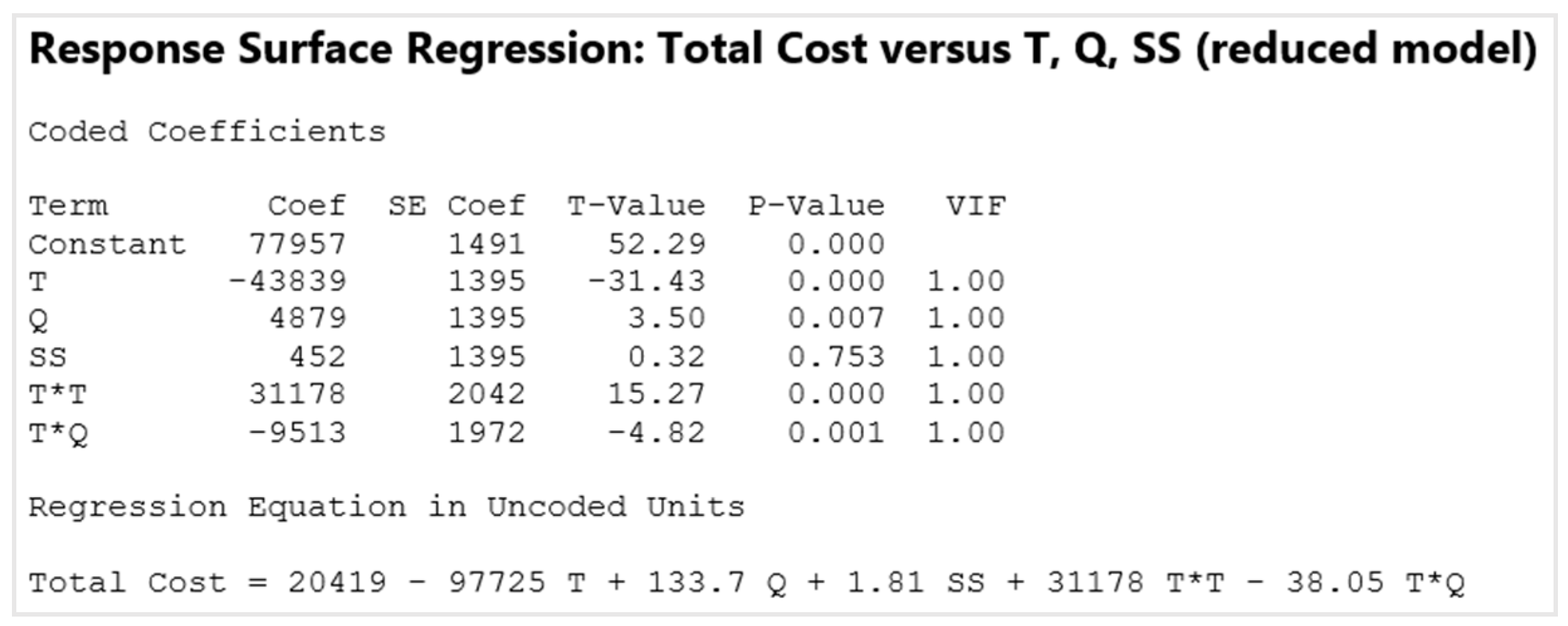
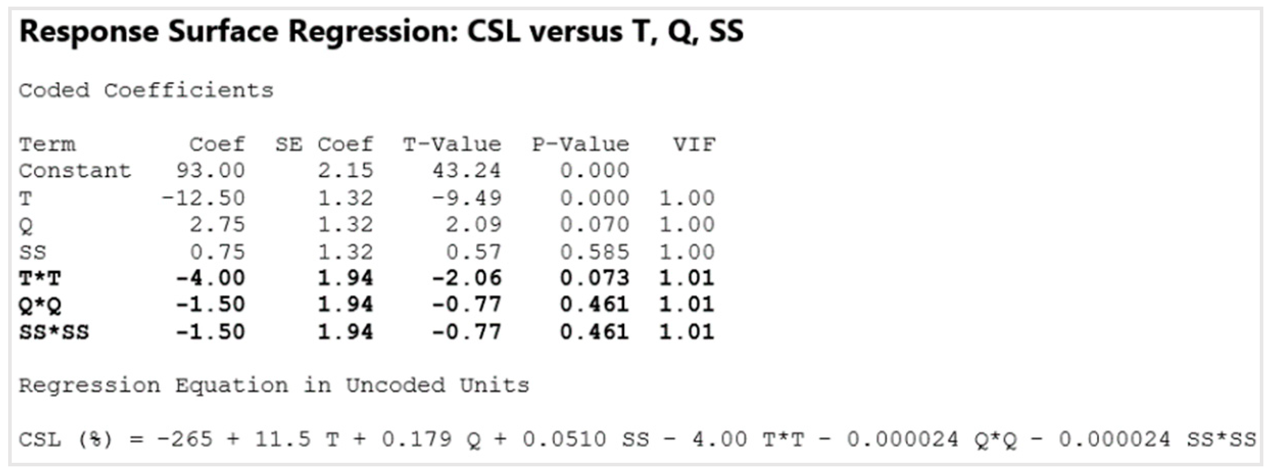
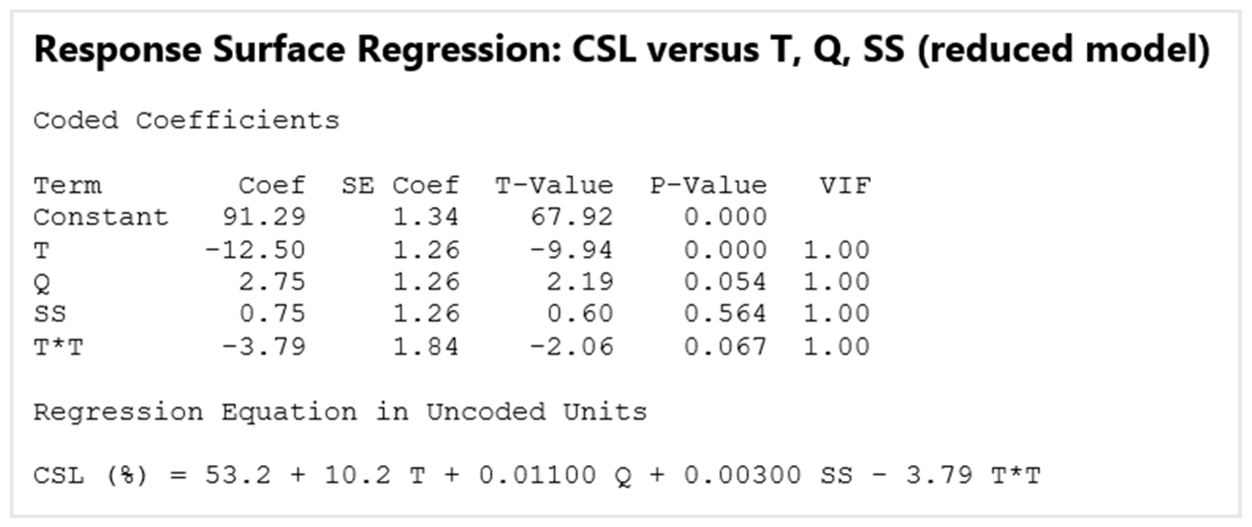
5.3. Central Composite Design (CCD)

In this section, a central composite design was performed to find the effects of independent variables on the response variables. In this paper, the CCD experiment (one continuous factor and two categorical factors) used the 20-run design with two blocks. Minitab provides the rotatability value (α) to ensure the design displays the desirable properties. The rotatability value of the CCD experiment was chosen based on factorial run and factorial point, α = 1.41 was applied in this experimental design. The CCD experiment running setup and randomized design table are presented in Figure 7 and

Table 5. Central composite design (one continuous factor and two categorical factors).

StdOrder	RunOrder	PtType	Blocks	T	Q	SS	TC	CSL
1	1	1	1	1	−1	−1	76,990.53	86
2	2	1	1	1	1	−1	78,115.85	93
3	3	1	1	1	−1	1	76,789.66	87
4	4	1	1	1	1	1	79,264.98	94
5	5	0	1	1	0	0	76,829.35	91
6	6	1	1	2	−1	−1	66,298.47	69
7	7	1	1	2	1	−1	64,918.34	78
8	8	1	1	2	−1	1	65,582.80	74
9	9	1	1	2	1	1	67,053.43	81
10	10	0	1	2	0	0	65,334.14	75
11	11	−1	2	1	−1.41	0	77,047.57	84
12	12	−1	2	1	1.41	0	96,797.76	94
13	13	−1	2	1	0	−1.41	76,971.17	90
14	14	−1	2	1	0	1.41	78,037.13	91
15	15	0	2	1	0	0	76,826.26	92
16	16	−1	2	2	−1.41	0	66,215.61	70
17	17	−1	2	2	1.41	0	74,732.52	81
18	18	−1	2	2	0	−1.41	65,732.97	73
19	19	−1	2	2	0	1.41	69,031.07	78
20	20	0	2	2	0	0	63,287.22	75

Note: calculated by the researchers.

below. Figure 7 shows all set-up parameters for the experimental CCD in the research. From the results of Table 5, TC and CSL were calculated based on independent variables, which T, Q, and SS. Note: StdOrder (standard order), RunOrder (run order), and PtType (center point type).

The initial experimental model was built for the response variables. Figure 8 shows the response surface regression of total cost versus T, Q, and SS. In the first running, the results suggest that the terms SS, the square terms SS*SS, and the interaction among Q*SS, Q*T, and SS*T were not significant (p-value > 0.05), and the paper considered the confidence level of the experimental design at 95%. In the next steps, these terms were eliminated from the CCD model.

After excluded these terms, the experiment was run once more. The results are shown in Figure 9, the reduced model. From the results, term T and the square term Q*Q were highly significant (p-value < 0.05), while term Q was barely significant. Thus, term Q was kept for the next analysis to see the effects of these independent variables on the objective functions.

For the second objective function, CSL (%), the CCD experiment was performed consequentially. The response surface regression of the CSL versus T, Q, and SS is presented in Figure 10. In the first running, the results display that the square terms SS*SS, and the interaction among Q*SS and Q*T was not significant (p-value > 0.05). Then, these terms were eliminated from the CCD model.

After excluded these terms, the CCD model was run again, the reduced model is shown in Figure 11. The results proposed that only the square term Q*Q was not significant because of the p-value = 0.068 was out of the confidence level at 95%. Meanwhile, the terms Q, SS, T, and the interaction of SS*T dramatically affected the CCD model (p-value < 0.05).

After reducing the CCD model into the final form, the residual plots for TC and CSL are displayed in Figure 12, including normal probability plot, histogram, versus fits, and versus order. The results show that the assumption of the model had no concern about the violation of the acceptable outliner. In detail, the normal probability plot nearly followed a straight line, then the residuals could assume from a normal distribution. The versus fits were used to verify that the residuals were scattered randomly about zero. From the plots, the non-constant variance of the residuals was fit. The histogram in the CCD model approximately followed a distribution. The versus order shows the residuals in the order of data collection. As can be seen, the versus order did not show any pattern, hence, there was no time correlation in the residuals.

Figure 13 shown the response optimizer of the CCD experiment to find the feasible response variables with CSL at 90% and 95%. From the result, the CSL set to target that was 90% with the possible minimum total cost 76,330 of the possible settings were T = 3, Q = 3428, and SS = 1336. Meanwhile, when the CSL was increased up to 95%, the possible minimum total cost was 77,090 of the optimal settings that were T = 3, Q = 3520, and SS = 1354.

Besides, the surface and contour plots for CSL are displayed in Figure 14. According to the contour plot, the CSL located in an area of dark green color was more satisfying. The trade-off existed in the objective function of the model. The more the customer service level is satisfied, the more of the total cost will be paid by the distributor.

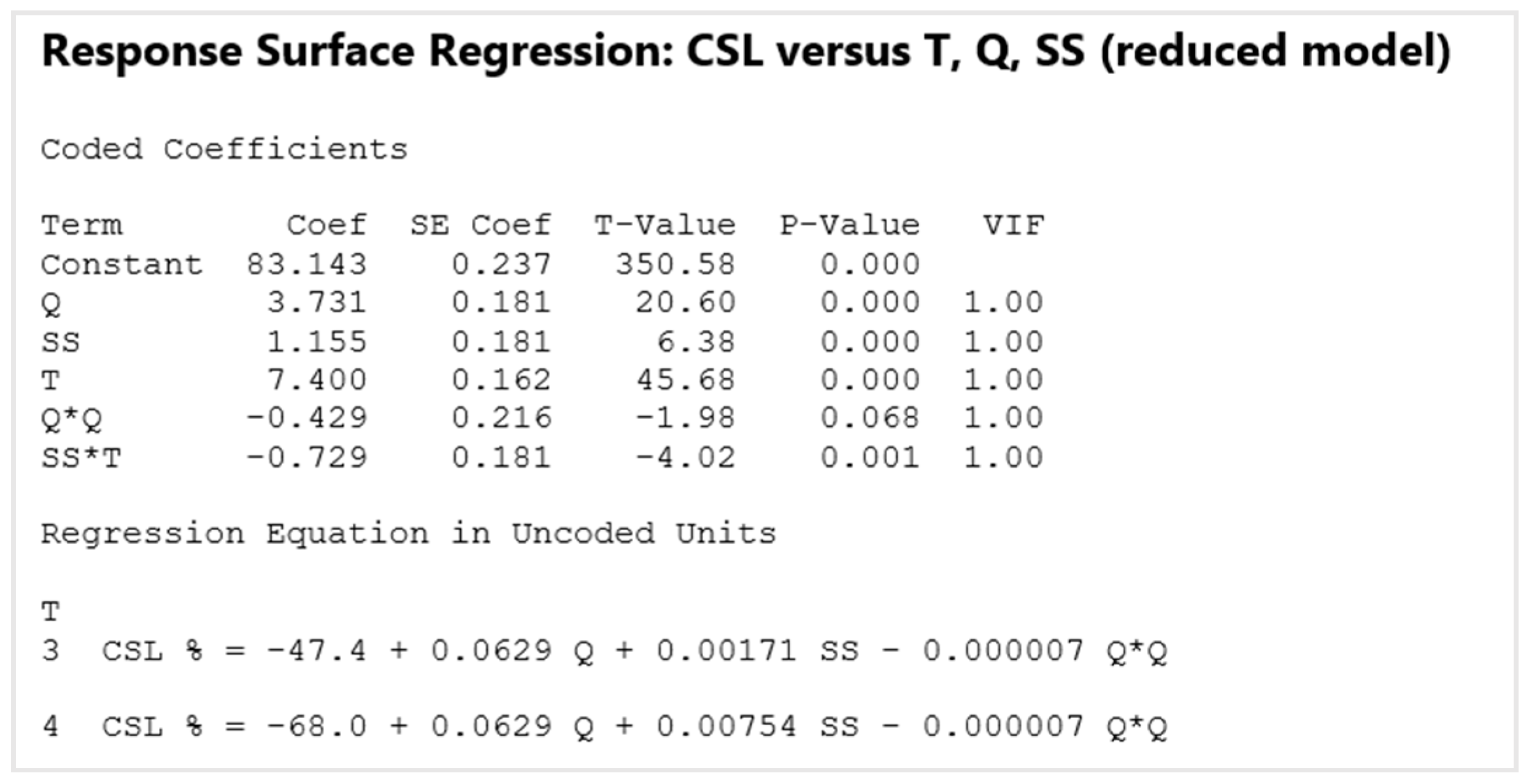
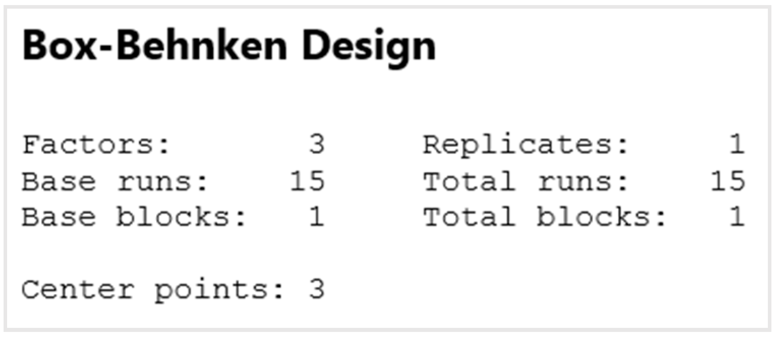
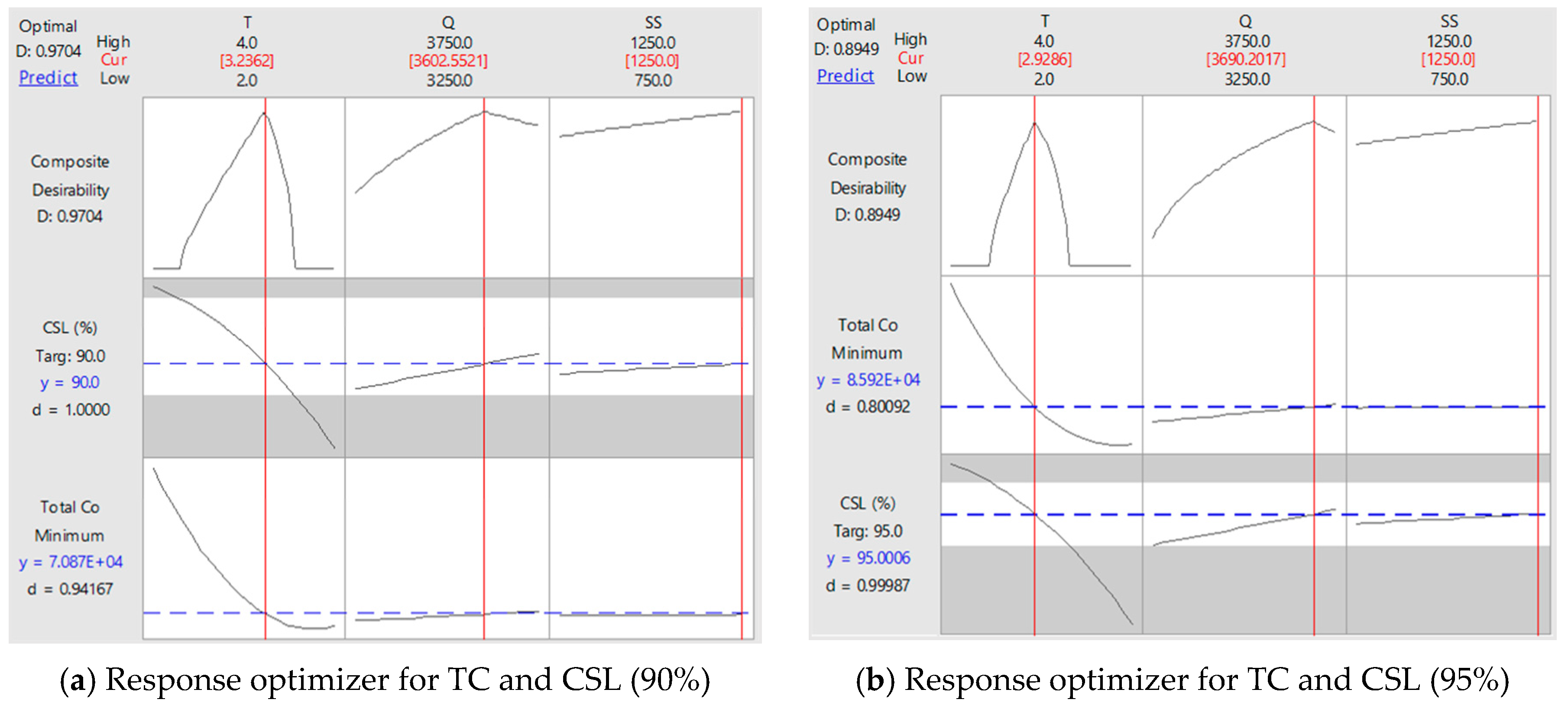
5.4. Box–Behnken Design (BBD)

Following the results from the experiment of the central composite design, Box–Behnken design was performed to compare the effects of independent variables on the response variables. In this experiment, BBD with three continuous factors used the total 15-run design with one block. Compared to the central composite design, the BBD experiment did not have an embedded factorial design and extreme points, and the BBD experiment also did not have the rotatability value (α) in the experimental design. The advantage of the BBD model was that the design usually had fewer design points, hence, they were often less expensive to run than the CCD design with the same number of independent variables. The BBD experiment running setup and randomized design table is presented in Figure 15 and

Table 6. Box–Behnken design (three continuous factors).

StdOrder	RunOrder	PtType	Blocks	T	Q	SS	TC	CSL
1	1	2	1	2	3250	1000	134,828.00	100
2	2	2	1	4	3250	1000	65,946.84	71
3	3	2	1	2	3750	1000	171,568.82	100
4	4	2	1	4	3750	1000	64,635.88	79
5	5	2	1	2	3500	750	151,097.12	100
6	6	2	1	4	3500	750	65,616.60	73
7	7	2	1	2	3500	1250	154,401.55	100
8	8	2	1	4	3500	1250	64,982.51	77
9	9	2	1	3	3250	750	76,990.53	86
10	10	2	1	3	3750	750	78,115.85	93
11	11	2	1	3	3250	1250	76,789.66	87
12	12	2	1	3	3750	1250	79,264.98	94
13	13	0	1	3	3500	1000	76,826.26	92
14	14	0	1	3	3500	1000	80,511.79	100
15	15	0	1	3	3500	1000	77,198.46	87

Note: calculated by the researchers.

as follows. Figure 15 shows all set-up parameters for the experimental BBD. From the results of Table 6, TC and CSL were calculated based on considered independent variables using an excel spreadsheet.

The initial model was obtained for the response variables (TC and CSL). Figure 16 shows the response surface regression of total cost versus T, Q, and SS. In the first running, the results suggest that the square terms Q*Q, SS*SS (p-values were 0.976 and 0.915 respectively), and the interaction among T*SS and Q*SS (p-values were 0.721 and 0.902, respectively) were not significant (all p-value > 0.05), while the paper considered the confidence level of the BBD at 95%. Then, these terms were eliminated from the BBD model to obtain the following final model.

After excluded insignificant terms, the experimental BBD was run again, the results of the reduced model are shown in Figure 17. The results display that term SS was statistically significant while the terms T, Q, square term T*T, and the interaction of T*Q significantly affected the model (p-value < 0.05). The authors decided to keep the term SS for further analysis to see the effects of these independent variables on the objective functions.

For the second objective function related to CSL (%), the BBD was performed consequentially. The response surface regression of the CSL versus T, Q, and SS is presented in Figure 18. In the first running, the results display that the term SS (p-value was 0.585) and the square terms Q*Q and SS*SS (p-values were 0.461 for both) were not significant (p-value > 0.05). In this case, the square terms Q*Q and SS*SS were eliminated from the BBD model in priority, the term SS was kept for further analysis purposes.

After excluded these terms, the BBD experiment was run again, the reduced model is shown in Figure 19. The results show that only the term Q, SS, and the square term T*T (p-values were 0.054, 0.564, and 0.067, respectively) were slightly significant because the p-value was slightly out of the confidence level at 95%. Otherwise, only the terms T was highly significant to the BBD experiment (p-value < 0.05).

After reducing the BBD model into the final form, the residual plots (normal probability plot, histogram, versus fits, and versus order plot) for the response variables (TC and CSL) are displayed in Figure 20. The results show that all residual plots satisfied the normality and constant variance assumptions, which means the simulated data was random and followed normal distribution.

Figure 21 shows the response optimizer of BBD to determine the feasible response variables, i.e., TC and CSL (CSL, 90%, 95%). From the result, the CSL set to target was 90% with the possible minimum total cost 70,870 of the possible settings were T = 3, Q = 3603, and SS = 1250. Otherwise, when the CSL was at 95%, the possible minimum total cost was 85,920 of the optimal settings were T = 3, Q = 3690, and SS = 1250.

Moreover, the surface and contour plots for CSL are shown in Figure 22. The results suggest that the possible minimum total cost was in an area of light green (<74,000), the area of SS less than 1000, and the area of Q was less than 3500 according to the contour plot. The trade-off existed in the objective function of the model, which means, the more the customer service level is satisfied, the more of the total cost will be paid by the distributor.

5.5. The Comparision of the CCD and BBD Experiment

This section performs the comparisons of the CCD and BBD experiments. The summary of the response optimizer results of CCD and BBD are displayed in

Table 7. The summary of the response optimizer results of CCD and BBD.

	Central Composite Design (CCD)		Box-Behnken Design (BBD)
	CSL (90%)	CSL (95%)	CSL (90%)	CSL (95%)
T	3	3	3	3
Q	3428	3520	3603	3690
SS	1336	1354	1250	1250
TC	76,330	77,090	70,870	85,920

Note: calculated by the researchers.

below. Next, the overlaid variance dispersion graph for CCD and BBD are drawn as in Figure 23. RSM was applied to build the prediction models, hence, prediction variance was significant. For more than two independent variables in the model, the variance dispersion graph (VDG) was one of the useful tools to validate the surface’s results. VDG shows the value of minimum, maximum, and average of the scaled prediction variance (SPV) versus the distance of the design point from the center point [50].

According to the terms of the variance in Figure 23, the blue lines show the BBD experiment while the green lines display the CCD experiment. Both of these designs almost had significant differences in the total cost results with 2000 difference, which means, the distance of design point from the center point, and the scaled prediction variance (SPV) shows the CCD design had better SPV (smallest values) than the BBD design, therefore, CCD experiment can be considered as the best model in this paper. On the other hand, based on the results of the response optimizer, BBD design gave the smallest total cost. In other words, this paper provided useful insights for reference decision-makers in the related industry. Based on the objective of the industry, the managers or policymakers can consider the possible experimental designs that give the best performance toward the strategy of sustainable development.

6. Discussions and Conclusions

This paper proposed a computational framework for the order planning problem in a distributor. In the proposed model, values of response variables were simulated and calculated, and Minitab was used to determine the possible optimal setting for those responses using the central composite design and Box–Behnken design. In the case study, a combination of the review period (T), order quantity (Q), and safety stock (SS) was selected as independent variables of the model. Additionally, the total cost of the holding cost, shortage cost, over-storage cost, and transportation cost, and customer service level was selected as response variables. The objective of the paper was to minimize the total cost by planning on placing the right order quantities, in the right periods, with the possible safety stock in order to reach customer satisfaction around 90–95 percent using RSM.

For solving an order planning problem of Spectite CW100, the statistical result from the factorial design shows that the curvature had a significant effect on the responses, therefore, two response surface designs, central composite design, and Box–Behnken design, were considered afterward to find the possible parameter settings. Based on the results in the response optimizer, the following values for the response surface design were as follows:

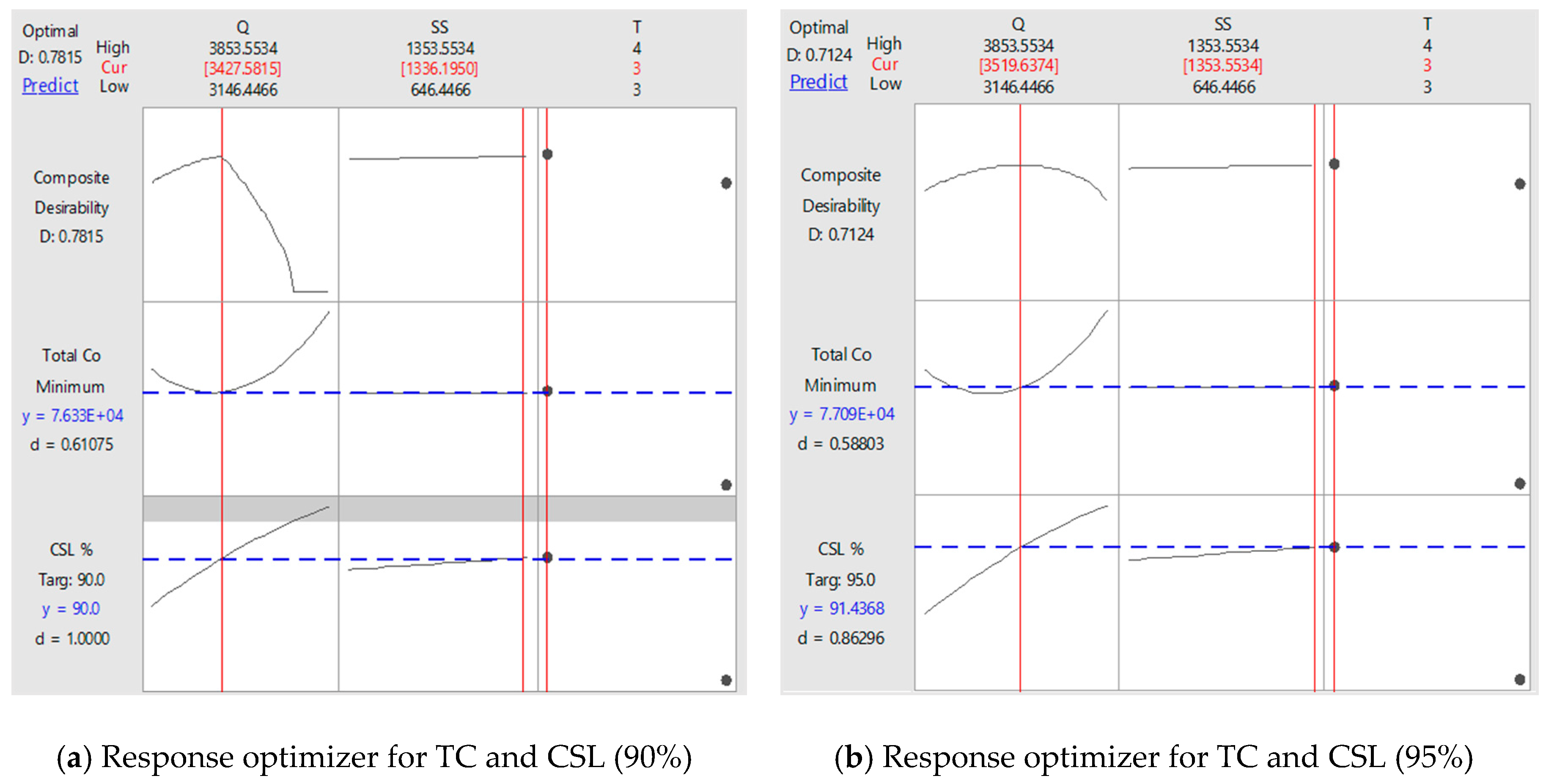
• Central composite design (CCD), customer service level CSL was at 90%, the minimum total cost was 76,330 with the possible optimal settings were the time period (T) = 3, order quantity (Q) = 3428, safety stock (SS) = 1336; (2) customer service level CSL was at 95%, the minimum total cost was 77,090 with the possible optimal settings were T = 3, Q = 3520, and SS = 1354.
• Box–Behnken design (BBD), customer service level CSL was at 90%, the minimum total cost was 70,870 with the possible optimal settings were the time period (T) = 3, order quantity (Q) = 3603, and safety stock (SS) = 1250; (2) customer service level CSL was at 95%, the minimum total cost was 85,920 with the possible optimal settings were T = 3, Q = 3690, and SS = 1250.

According to the scaled prediction variance (SPV), the CCD design had better SPV (smallest values) than the BBD design, therefore, the CCD experiment could be considered as the best model in this paper. On the other hand, based on the results of the response optimizer, BBD design gave the smallest total cost. When the CSL increased from 90% to 95%, the total cost also increased in both designs. The proposed computational framework can be applied to other products of the distributor (Spectite WS, Spectite HP600, and Speccoat PE145), or any ordering process in businesses within the supply chain. In summary, our contributions include (1) the paper proposed a computational framework to solve the order planning problem by a heuristics approach using RSM, (2) the model was tested with a case study of a distributor to show the model’s effectiveness, and (3) The insights implication of the model’s results was to provide a useful reference for purchasing managers or decision-makers to obtain the most suitable order policy for a robust order planning process, which includes responses that were considered in monetary values. Besides, this could be used as a guideline for other related industries. However, there were some limitations to this paper. To get more robust solutions, future studies should consider considerable data on the products and address this problem under stochastic demand, lead time uncertainty, and unstable markets.

References

1. Designing Building Wiki. Supply Chain Management in Construction. Available online: https://www.designingbuildings.co.uk/wiki/Supply_chain_management_in_construction#The_need_for_SCM_in_construction (accessed on 31 November 2020).
2. Right Place, Right Time: The Importance of Order-Slotting Solutions. Available online: https://blog.flexis.com/right-place-right-time-the-importance-of-order-slotting-solutions (accessed on 31 November 2020).
3. Cavalcante, C.A. Order planning policies for business-to-consumer e-tail stores. Comput. Ind. Eng. 2019, 136, 106–116. [Google Scholar]
4. Chien, C.F.; Lin, Y.S.; Lin, S.K. Deep reinforcement learning for selecting demand forecast models to empower Industry 3.5 and an empirical study for a semiconductor component distributor. Int. J. Prod. Res. 2020, 58, 2784–2804. [Google Scholar] [CrossRef]
5. Geunes, J.; Akçali, E.; Pardalos, P.M.; Romeijn, H.E.; Shen, Z.J.M. (Eds.) Applications of Supply Chain Management and e-Commerce Research; Springer Science & Business Media: Berlin, Germany, 2006; Volume 92. [Google Scholar]
6. Partovi, F.Y.; Anandarajan, M. Classifying inventory using an artificial neural network approach. Comput. Ind. Eng. 2002, 41, 389–404. [Google Scholar] [CrossRef]
7. Yao, X.; Huang, R.; Song, M.; Mishra, N. Pre-positioning inventory and service outsourcing of relief material supply chain. Int. J. Prod. Res. 2018, 56, 6859–6871. [Google Scholar] [CrossRef]
8. Diabat, A.; Abdallah, T.; Le, T. A hybrid tabu search based heuristic for the periodic distribution inventory problem with perishable goods. Ann. Oper. Res. 2016, 242, 373–398. [Google Scholar] [CrossRef]
9. Diabat, A.; Deskoores, R. A hybrid genetic algorithm based heuristic for an integrated supply chain problem. J. Manuf. Syst. 2016, 38, 172–180. [Google Scholar] [CrossRef]
10. Clark, A.J.; Scarf, H. Optimal policies for a multi-echelon inventory problem. Manag. Sci. 1960, 6, 475–490. [Google Scholar] [CrossRef]
11. Gharaei, A.; Pasandideh, S.H.R.; Khamseh, A.A. Inventory model in a four-echelon integrated supply chain: Modeling and optimization. J. Model. Manag. 2017, 12, 739–762. [Google Scholar] [CrossRef]
12. Hoseini Shekarabi, S.A.; Gharaei, A.; Karimi, M. Modelling and optimal lot-sizing of integrated multi-level multi-wholesaler supply chains under the shortage and limited warehouse space: Generalised outer approximation. Int. J. Syst. Sci. Oper. Logist. 2019, 6, 237–257. [Google Scholar] [CrossRef]
13. Ben-Daya, M.; Hariga, M. Integrated single vendor single buyer model with stochastic demand and variable lead time. Int. J. Prod. Econ. 2004, 92, 75–80. [Google Scholar] [CrossRef]
14. Jauhari, W.A.; Laksono, P.W. A joint economic lot-sizing problem with fuzzy demand, defective items and environmental impacts. Mater. Sci. Eng. 2017, 273, 12–18. [Google Scholar] [CrossRef]
15. Kao, C.; Hsu, W.K. A single-period inventory model with fuzzy demand. Comput. Math. Appl. 2002, 43, 841–848. [Google Scholar] [CrossRef] [Green Version]
16. Kim, G.; Wu, K.; Huang, E. Optimal inventory control in a multi-period newsvendor problem with non-stationary demand. Adv. Eng. Inform. 2015, 29, 139–145. [Google Scholar] [CrossRef]
17. Modak, N.M.; Panda, S.; Sana, S.S.; Basu, M. Corporate social responsibility, coordination and profit distribution in a dual-channel supply chain. Pac. Sci. Rev. 2014, 16, 235–249. [Google Scholar] [CrossRef] [Green Version]
18. Modak, N.M.; Panda, S.; Sana, S.S. Pricing policy and coordination for a two-layer supply chain of duopolistic retailers and socially responsible manufacturer. Int. J. Logist. Res. Appl. 2016, 19, 487–508. [Google Scholar] [CrossRef]
19. Modak, N.M.; Panda, S.; Sana, S.S. Pricing policy and coordination for a distribution channel with manufacturer suggested retail price. Int. J. Syst. Sci. Oper. Logist. 2016, 3, 92–101. [Google Scholar] [CrossRef]
20. Modak, N.M.; Panda, S.; Sana, S.S. Three-echelon supply chain coordination considering duopolistic retailers with perfect quality products. Int. J. Prod. Econ. 2016, 182, 564–578. [Google Scholar] [CrossRef]
21. Modak, N.M.; Panda, S.; Sana, S.S. Two-echelon supply chain coordination among manufacturer and duopolies retailers with recycling facility. Int. J. Adv. Manuf. Technol. 2016, 87, 1531–1546. [Google Scholar] [CrossRef]
22. Modak, N.M.; Modak, N.; Panda, S.; Sana, S.S. Analyzing structure of two-echelon closed-loop supply chain for pricing, quality and recycling management. J. Clean. Prod. 2018, 171, 512–528. [Google Scholar] [CrossRef]
23. Wang, C.-N.; Dang, T.-T.; Le, T.Q.; Kewcharoenwong, P. Transportation Optimization Models for Intermodal Networks with Fuzzy Node Capacity, Detour Factor, and Vehicle Utilization Constraints. Mathematics 2020, 8, 2109. [Google Scholar] [CrossRef]
24. Chilmon, B.; Tipi, N.S. Modelling and simulation considerations for an end-to-end supply chain system. Comput. Ind. Eng. 2020, 150, 106870. [Google Scholar] [CrossRef]
25. Tordecilla, R.D.; Juan, A.A.; Montoya-Torres, J.R.; Quintero-Araujo, C.L.; Panadero, J. Simulation-optimization methods for designing and assessing resilient supply chain networks under uncertainty scenarios: A review. Simul. Model. Pract. Theory 2020, 106, 102166. [Google Scholar] [CrossRef]
26. Shaban, A.; Shalaby, M.A. Modeling and optimizing of variance amplification in supply chain using response surface methodology. Comput. Ind. Eng. 2018, 120, 392–400. [Google Scholar] [CrossRef]
27. Giddings, A.P.; Bailey, T.G.; Moore, J.T. Optimality analysis of facility location problems using response surface methodology. Int. J. Phys. Distrib. Logist. Manag. 2001, 31, 38–52. [Google Scholar] [CrossRef]
28. Shang, J.S.; Li, S.; Tadikamalla, P. Operational design of a supply chain system using the Taguchi method, response surface methodology, simulation, and optimization. Int. J. Prod. Res. 2004, 42, 3823–3849. [Google Scholar] [CrossRef]
29. Buchholz, P.; Müller, D.; Thümmler, A. Optimization of process chain models with response surface methodology and the ProC/B toolset. In Supply Chain Management und Logistik; Physica-Verlag HD: Heidelberg, Germany, 2005; pp. 553–575. [Google Scholar]
30. Hassanzadeh, A.; Jafarian, A.; Amiri, M. Modeling and analysis of the causes of bullwhip effect in centralized and decentralized supply chain using response surface method. Appl. Math. Model. 2014, 38, 2353–2365. [Google Scholar] [CrossRef]
31. Devika, K.; Jafarian, A.; Hassanzadeh, A.; Khodaverdi, R. Optimizing of bullwhip effect and net stock amplification in three-echelon supply chains using evolutionary multi-objective metaheuristics. Ann. Oper. Res. 2016, 242, 457–487. [Google Scholar] [CrossRef]
32. Tang, L.; Yang, T.; Ma, Y.; Wang, J. Analysis of bullwhip effect and the robustness of supply chain using a hybrid Taguchi and dual response surface method. In Proceedings of the 2017 International Conference on Service Systems and Service Management, Dalian, China, 16–18 June 2017; pp. 1–6. [Google Scholar]
33. Zhang, T.; Zheng, Q.P.; Fang, Y.; Zhang, Y. Multi-level inventory matching and order planning under the hybrid Make-To-Order/Make-To-Stock production environment for steel plants via Particle Swarm Optimization. Comput. Ind. Eng. 2015, 87, 238–249. [Google Scholar] [CrossRef]
34. Guo, Z.X.; Yang, C.; Wang, W.; Yang, J. Harmony search-based multi-objective optimization model for multi-site order planning with multiple uncertainties and learning effects. Comput. Ind. Eng. 2015, 83, 74–90. [Google Scholar] [CrossRef]
35. Lim, L.L.; Alpan, G.; Penz, B. A simulation-optimization approach for sales and operations planning in build-to-order industries with distant sourcing: Focus on the automotive industry. Comput. Ind. Eng. 2017, 112, 469–482. [Google Scholar] [CrossRef]
36. Singha, K.; Buddhakulsomsiri, J.; Parthanadee, P. Mathematical model of inventory policy under limited storage space for continuous and periodic review policies with backlog and lost sales. Math. Probl. Eng. 2017, 2017, 1–9. [Google Scholar] [CrossRef]
37. Jansen, S.; Atan, Z.; Adan, I.; de Kok, T. Setting optimal planned leadtimes in configure-to-order assembly systems. Eur. J. Oper. Res. 2019, 273, 585–595. [Google Scholar] [CrossRef]
38. Kokuryo, D.; Yamashita, K.; Kaihara, T.; Fujii, N.; Umeda, T.; Izutsu, R. A proposed production decision method for order planning considering decision criteria of multiple organizations. Procedia CIRP 2020, 93, 933–937. [Google Scholar] [CrossRef]
39. Thinakaran, N.; Jayaprakas, J.; Elanchezhian, C. Survey on inventory model of EOQ & EPQ with partial backorder problems. Mater. Today Proc. 2019, 16, 629–635. [Google Scholar]
40. Tai, P.; Huyen, P.; Buddhakulsomsiri, J. A novel modeling approach for a capacitated (S,T) inventory system with backlog under stochastic discrete demand and lead time. Int. J. Ind. Eng. Comput. 2020, 12, 1–14. [Google Scholar] [CrossRef]
41. Hunsucker, J.L.; Shah, J.R. Performance of priority rules in a due date flow shop. Omega 1992, 20, 73–89. [Google Scholar] [CrossRef]
42. Wang, C.-N.; Dang, T.-T.; Nguyen, N.-A.-T. A computational model for determining levels of factors in inventory management using response surface methodology. Mathematics 2020, 8, 1210. [Google Scholar] [CrossRef]
43. Myers, R.H.; Montgomery, D.C.; Cook, C.M.A. Response Surface Methodology: Process and Product Optimization Using Designed Experiments, 3rd ed.; John Wiley & Sons: Hoboken, NJ, USA, 2009; Volume 39. [Google Scholar]
44. Khuri, A.I. Response surface methodology and its applications in agricultural and food sciences. Int. J. Biom. Biostat. 2017, 5, 1–11. [Google Scholar] [CrossRef] [Green Version]
45. Goh, T.N. The role of statistical design of experiments in six sigma: Perspectives of a practitioner. Qual. Eng. 2002, 14, 659–671. [Google Scholar] [CrossRef]
46. Shi, W.; Shang, J.; Liu, Z.; Zuo, X. Optimal design of the auto parts supply chain for JIT operations: Sequential bifurcation factor screening and multi-response surface methodology. Eur. J. Oper. Res. 2014, 236, 664–676. [Google Scholar] [CrossRef]
47. Widodo, E. A review of response surface methodology approach in supply chain management. In Proceedings of the 3rd Asia Pacific Conference on Research in Industrial and Systems Engineering, Depok, Indonesia, 16–17 June 2020; pp. 322–327. [Google Scholar]
48. Radasanu, A.C. Inventory management, service level and safety stock. J. Public Adm. Financ. Law 2016, 9, 145–153. [Google Scholar]
49. Coleman, B.J. Determining the correct service level target. Prod. Inventory Manag. J. 2000, 41, 19. [Google Scholar]
50. Montgomery, D.C. Design and Analysis of Experiments; John Wiley & Sons: Hoboken, NJ, USA, 2017. [Google Scholar]
Figure 1. The experimental runs of the central composite design (CCD) and Box–Behnken design (BBD).
Applsci 10 08959 g001
Figure 2. A computational framework.
Applsci 10 08959 g002
Figure 3. List of the main materials group of the distributor.
Applsci 10 08959 g003
Figure 4. Excel spreadsheet simulation.
Applsci 10 08959 g004
Figure 5. Analysis of variance of factorial regression.
Applsci 10 08959 g005
Figure 6. Pareto chart of the standardized effects.
Applsci 10 08959 g006
Figure 7. Central composite design running setup.
Applsci 10 08959 g007
Figure 8. CCD—response surface regression of total cost (TC) versus the period (T), order quantity (Q), and safety stock (SS).
Applsci 10 08959 g008
Figure 9. CCD—response surface regression of TC versus T, Q, and SS (reduced model).
Applsci 10 08959 g009
Figure 10. CCD—response surface regression of the customer service level (CSL; %) versus T, Q, and SS.
Applsci 10 08959 g010
Figure 11. CCD—response surface regression of CSL (%) versus T, Q, and SS (reduced model).
Applsci 10 08959 g011
Figure 12. CCD—residual plots for TC and CSL.
Applsci 10 08959 g012
Figure 13. CCD—response optimizer for TC and CSL.
Applsci 10 08959 g013
Figure 14. CCD—surface and contour plots for CSL (%).
Applsci 10 08959 g014
Figure 15. Box–Behnken design running setup.
Applsci 10 08959 g015
Figure 16. BBD—response surface regression of TC versus T, Q, and SS.
Applsci 10 08959 g016
Figure 17. BBD—response surface regression of TC versus T, Q, and SS (reduced model).
Applsci 10 08959 g017
Figure 18. BBD—response surface regression of CSL (%) versus T, Q, and SS.
Applsci 10 08959 g018
Figure 19. BBD—response surface regression of CSL (%) versus T, Q, and SS (reduced model).
Applsci 10 08959 g019
Figure 20. BBD—residual plots for TC and CSL.
Applsci 10 08959 g020
Figure 21. BBD—response optimizer for TC and CSL.
Applsci 10 08959 g021
Figure 22. BBD—surface and contour plots for the total cost.
Applsci 10 08959 g022
Figure 23. Variance dispersion graph for the CCD and BBD experiment.
Applsci 10 08959 g023