Article

Susceptibility Mapping on Urban Landslides Using Deep Learning Approaches in Mt. Umyeon

1
Department of Geoinformatics, University of Seoul, 163 Seoulsiripdaero, Dongdaemun-gu, Seoul 02504, Korea
2
Center for Environmental Assessment Monitoring, Environmental Assessment Group, Korea Environment Institute (KEI), Sejong-si 30147, Korea
3
Geoscience Platform Division, Korea Institute of Geoscience and Mineral Resources (KIGAM), 124 Gwahak-ro, Yuseong-gu, Daejeon 34132, Korea
4
Department of Geophysical Exploration, Korea University of Science and Technology, 217 Gajeong-ro, Yuseong-gu, Daejeon 34113, Korea
*
Authors to whom correspondence should be addressed.
Appl. Sci. 2020, 10(22), 8189; https://doi.org/10.3390/app10228189
Submission received: 30 September 2020 / Revised: 6 November 2020 / Accepted: 17 November 2020 / Published: 19 November 2020
(This article belongs to the Special Issue Machine Learning Techniques Applied to Geospatial Big Data)

Abstract

:
In recent years, the incidence of localized heavy rainfall has increased as abnormal weather events occur more frequently. In densely populated urban areas, this type of heavy rain can cause extreme landslide damage, so that it is necessary to estimate and analyze the susceptibility of future landslides. In this regard, deep learning (DL) methodologies have been used to identify areas prone to landslides recently. Therefore, in this study, DL methodologies, including a deep neural network (DNN), kernel-based DNN, and convolutional neural network (CNN) were used to identify areas where landslides could occur. As a detailed step for this purpose, landslide occurrence was first determined as landslide inventory through aerial photographs with comparative analysis using field survey data; a training set was built for model training through oversampling based on the landslide inventory. A total of 17 landslide influencing variables that influence the frequency of landslides by topography and geomorphology, as well as soil and forest variables, were selected to establish a landslide inventory. Then models were built using DNN, kernel-based DNN, and CNN models, and the susceptibility of landslides in the study area was determined. Model performance was evaluated through the average precision (AP) score and root mean square error (RMSE) for each of the three models. Finally, DNN, kernel-based DNN, and CNN models showed performances of 99.45%, 99.44%, and 99.41%, and RMSE values of 0.1694, 0.1806, and 0.1747, respectively. As a result, all three models showed similar performance, indicating excellent predictive ability of the models developed in this study. The information of landslides occurring in urban areas, which cause a great damage even with a small number of occurrences, can provide a basis for reference to the government and local authorities for urban landslide management.

1. Introduction

Natural disasters are becoming more frequent around the world due to extreme climates, and an increase in the probability of extreme rain is also associated with the occurrence of damage. In Korea, the current rainfall and rainfall intensity have gradually increased compared to the past, and the rainfall is concentrated in a small area over a short time. A lot of water-related disaster damage has occurred in this localized heavy rain, but the damage is also decreasing due to continuous river maintenance and the installation of facilities to prevent flooding. On the other hand, the number of casualties, 134 people, caused by landslides and slope failures has not decreased since the 2000s [1]. Recently, the incidence of localized rainfall increased 2.4 times, from an average of 5.1 in the 1970s to 12.3 in the 2000s [2]. Due to the increase in localized heavy rain, landslides and geomorphological hazards, such as debris flows, are rapidly increasing [3].
Landslides in Korea occur intensively in June to September, when heavy rains and typhoons occur, costing many lives and significant property damage. The area of landslide damage since the 2000s has been more than three times that of the 1980s [4]. In particular, serious damage to human lives has occurred in the years of torrential rains and typhoons, which is a serious social issue [5]. This kind of phenomenon is occurring not only in Korea, but also in other parts of the world, raising concerns about the occurrence of landslides. Damage increases due to a combination of natural and artificial causes; the increase in localized heavy rain is an example of a natural cause, and an indiscriminate development is a representative artificial cause. Development projects in mountainous regions have increased due to the tendency to prefer a nature-friendly environment. The risk of landslides is increasing due to the increasing number of cases where residential facilities, such as apartments, are located near steep slopes.
When torrential rainfall occurs, the soil begins to be saturated, the pore pressure increases, and the shear strength decreases. In addition, when rainfall infiltrates the bedrock, the adhesive strength weakens. The possibility of landslides increases when the soil is not able to support the increased weight of the saturated soil. Artificial steep slopes have the same characteristics; the expected damage range is a horizontal distance equal to twice the height of the slope. The steep slope in an urban area needs essential management for reducing the risk from landslides. In particular, debris flow is a phenomenon in which debris, such as rock fragments, soil, and mud move in groups with high speed. The debris, clay and rocks increase its volume and flow with strong erosion power, so that debris flow is the most dangerous type of landslide; research on debris flow is being conducted in various aspects [6,7,8]. It could lead to a large-scale disaster, with a loss of roads and damage to houses and people, especially when it occurs in urban areas.
In order to prevent or minimize damage from debris flow, it is important to install disaster prevention facilities by predicting movement paths and sedimentary areas before the event [9]. A debris barrier is a fundamental way to protect people and property from debris flow, but it is practically impossible to install it in all dangerous paths. Also, there are the difficulties related to modeling debris flows, due to the uncertainties in defining debris flow rheology behavior, such as the transition from a quasi-static regime to liquid regime [10]. The effects of grain concentration could lead to a dilatant or pseudoplastic fluid behavior, depending on grain volume concentration [11]; finally, the presence of coarse sediment fraction could affects both yield stress and the transition between solid-like to fluid-like behavior [12]. Therefore, it is more efficient to install facilities by predicting the extent of damage to the debris flow [13,14]. Landslide susceptibility analysis not only analyzes the cause of landslide occurrence, but also estimates the susceptibility of future occurrence, so it can be effectively used to prevent landslides in advance [15]. Accordingly, research on the susceptibility of landslides has been actively conducted by researchers.
Since a geographic information system (GIS) provides integrated analysis of various spatial data, it is useful to effectively analyze complex interrelationships between landslides and landslide-related variables. For this reason, there have been many attempts to explain the spatial pattern with various models based on GIS, in order to analyze the susceptibility of landslide occurrences in recent years. Most of the information for landslide prevention can come from modeling efforts using predictive models. Traditionally, to evaluate the susceptibility of landslide occurrence, simple, statistics-based frequency ratio (FR) [16,17,18] and logistic regression (LR) [19,20,21] were proposed and used as a representative prediction model. In recent years, various attempts have been made to produce machine learning (ML) models, such as support vector machines [22,23], artificial neural networks (ANNs) [24,25,26], ensembles [27,28], or hybrid models [29,30] including neuro-fuzzy [31,32] or metaheuristic ones [33,34]. Several spatial modeling studies were conducted on areas where landslides could occur in various regions by using these models with GIS [35,36].
In recent years, deep learning (DL), one of the ML technologies, has been receiving a lot of attention since it shows reliable results similar to or better than the existing ML methods [37]. In particular, it has been shown that model architectures, such as deep neural networks (DNNs), which are widespread, can significantly improve the quality of results [38]. In the area of landslide research, DL algorithms have mostly been used for landslide detection [39,40,41,42]. Additionally, among various DL methods, convolutional neural networks (CNNs) can identify expressions with extreme variability through convolution and pooling layers [43]. As a result, CNNs can play an important role in susceptibility analysis, as they can remove tedious functional engineering steps and extract useful information directly from the original data.
Although various techniques have been used, there is no academic consensus on which technique is most effective. Therefore, it is important to improve the accuracy of landslide susceptibility analysis by conducting comparative studies using various techniques, or by integrating multiple models [44,45]. Therefore, in this study, we tried to build this effort by using and comparing DL methodologies to map the susceptibility of landslides in the Mt. Umyeon area of Seoul, Korea. To this end, DNN, kernel-based DNN, and CNN models were applied among the DL models. This study proposes the application of DNNs for estimating landslide susceptibility, and compares their predictive ability with other models of ML techniques.

2. Study Area and Data

2.1. Study Area

As shown in Figure 1, the study area is Mt. Umyeon, located in Seocho-gu, Seoul. Seoul is the largest city in Korea (about 605 km2), located in the center of the Korean Peninsula, and is one of the most populous cities in the world. This city, with about 10 million citizens, has a complex transportation and social infrastructure system. This density allows natural disasters, including landslides, to cause more recurrent disasters and serious damage [46]. The study area, Mt. Umyeon, is also a shallow mountain, with a height of 321.6 m, located in the center of a complex in a large city.
The slope near the summit is about 30 degrees, and most areas are less than 15 degrees. There is a gneissic rock outcrop in the area from weathering and geomorphological process. The biotite gneiss is weak to weathering, which could increase the susceptibility of debris flow in the area. The soil composition of this study area is mainly the brown forest soil developed on the parent rocks of biotite gneiss and granite gneiss. In some valley areas of the study area, brown forest soils with deep soil depth and high organic content are distributed, and the soil texture is silt and silt loam of sand, which drains well and easily causes severe weathering of the surface.
In July 2011, Typhoons Muifa and Kompasu generated 1092 mm of rainfall in Seoul for a month, and this resulted in simultaneous debris flows in the Mt. Umyeon area of Seoul. Specifically, 588 mm of heavy rain, which is about 40% of the annual average rainfall of 1451 mm, was concentrated in Mt. Umyeon for 3 days from July 26 to 28; debris flows caused 16 casualties and dozens of houses were damaged [47]. Debris flows that occurred simultaneously around Mt. Umyeon poured into streets and residential areas in downtown Seoul, damaging to apartments, vehicles, and pedestrians under the mountain, causing damage to life and property [48,49]. As shown in Figure 1, the debris flow of Mt. Umyeon occurred in the middle of the downtown area, different from the damage that occurred in the existing mountainous areas; the ripple effect was much greater than that in the past. This can be seen as a representative example, showing that even urban areas are not safe zones when a landslide, especially debris flow, occurs due to heavy rains [50,51].

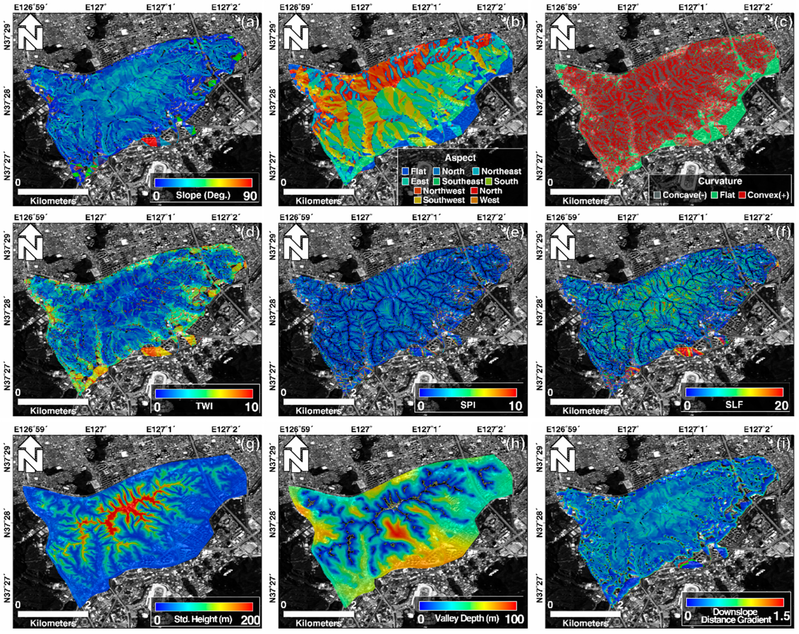
2.2. Spatial Datasets

In applying the data-driven methodology based on the established landslide (of debris flow in this study area) locations, accurate data is essential to build an appropriate database. In this study, data on the location of landslides was acquired based on aerial photographs. Additionally, 17 variables were selected as landslide-related variables; the variables were selected by referring to previous studies on various aspects of landslides, as follows: nine topographical variables (slope, aspect, curvature, topographic wetness index (TWI), stream power index (SPI), slope length factor (SLF), standardized height, valley depth, and downslope distance gradient (DDG)), four forest variables (timber type, timber diameter, timber density, and timber age) and four soil variables (soil depth, soil drainage, soil topography, and soil texture). The variables were selected as correlating between the landslides, and the variables have been investigated through the frequency ratio model in previous research [46,52,53].
Landslides in the Mt. Umyeon area received a lot of attention because damage occurred in areas where human activity was high, including major roads and residential areas in Seoul. Accordingly, a large-scale investigation into the cause and damage was conducted, so that a large amount of data, such as aerial photographs and field survey data, have been accumulated. Aerial photographs provide accurate status on the condition of the surface, with effectively captured complex urban structures. Also, despite the high cost of aerial photography, continuous monitoring using images is cost-effective for dense urban areas. The data on the location of landslides were selected by comparing the aerial photographs of Mt. Umyeon in 2010 before the occurrence and immediately after the occurrence in 2011 (Figure 2). Starting with the loss of the top slope, a debris flow occurred in which rocks and waste wood contained in the weathering and debris layers were lost together [54]. Accordingly, the landslide occurrence point was extracted based on the landslide occurrence starting point in this study, as in previous studies [27,31,55]. The traces of landslides in Mt. Umyeon remain for several years after the occurrence of debris flow, so it was easy to obtain through aerial photographic analysis. In addition, overlay and comparative analysis of 1:5000 digital topographic maps were performed, and 103 starting points of the landslide from landslide inventory were finally determined by comparing it with field survey data [56] conducted by the Seoul Metropolitan Government.
Slopes have an important effect on the occurrence of landslides, as they affect water flow and soil characteristics [46,57]. Slope is a main landslide influencing factor that has the greatest impact on landslides, in that gentle slopes tend to have a lower frequency of landslides [55,58]. Therefore, the input layer for landslide susceptibility analysis was constructed by focusing on topographic and geomorphlogic variables among the variables that influence landslides (Figure 3). The topographic variables were calculated based on the acquisition of a digital topographic map (1:5000) generated by the National Geographic Information Institute (NGII); the slope was calculated using ArcGIS software (ESRI, Redlands, LA, United States) after geometric correction (Figure 3a), and the following additional topographic and geomorphologic variables were calculated using SAGA (Automated Geoscientific Analyses) GIS [59].
Slope aspect was classified into flat and north, northeast, east, southeast, south, southwest, west, and northwest, with 25 degree intervals (Figure 3b). The curvature variable represents the morphological characteristics of the research area by expressing the upwardly convex surface as a positive value, and the upwardly concave surface as a negative value. Curvature, a morphological characteristic in terms of affecting the erosion process and landslide evolution, is commonly used in landslide analysis, because it can account for local surface relief in the study area [58,60] (Figure 3c). TWI was used to express the influence of terrain on the presence of a runoff-generated saturated area [61,62], with higher values increasing the probability of landslide occurrence (Figure 3d) [63]. The erosive power of surface flow, measured by the SPI index, is one of the variables that influence landslides [64]. Higher SPI values indicate an increased likelihood of erosion that affects local stability [61], and allows a general determination of where soil conservation is needed to reduce the effects of surface runoff erosion (Figure 3e) [61]. SLF values refer to the ratio of soil loss to slope length, and were calculated through the revised universal soil loss equation (Figure 3f) [65]. The standardized height is calculated by multiplying the absolute height by the height of the study area normalized between 0 and 1 (Figure 3g). The standardized height yields parameters suitable for soil property prediction by simplifying complex terrain conditions using linear regression [66]. The standardized height represents a value suitable for predicting soil properties, by simplifying complex terrain conditions using linear regression [66]. Valley depth means the vertical distance at the basic level of the channel network [59]; valley depth has been used as a landslide-influencing variable in several studies (Figure 3h) [46,67]. The DDG is determined through quantitative hydrological gradient estimation and the downslope distance calculation when water loses a determined amount of energy due to precipitation (Figure 3i) [68].
The vegetation provides root strength to help stabilize the mountain slope. The effect of rainfall on the slope is likely to be mitigated by the degree of vegetation distribution. The attributes selected by several studies as landslide-influencing variables, including timber diameter, type, density, and age, were extracted from a digital vegetation map with a ratio of 1:25,000, provided by the Korea Forest Service (Figure 4a–d). As reported in numerous additional studies, landslides are strongly influenced by the geological structure and soil type covering the area [69,70]. Geological cover is one of the most used variables in the assessment of landslide susceptibility [58]; however, in this study, it was excluded, because it was mostly the same due to the size of the study area. Physical and organizational soil cover properties influence surface runoff and penetration processes [71]. Soil properties affect the flow of water, including surface and groundwater, in the way that landslides occur when the amount of water in the soil exceeds the drainage capacity and the cohesion drops sharply [72]. Therefore, forest and soil characteristics were considered as landslide-influencing variables in this study (Figure 4) [46]. Each variable was pre-processed into raster format with a grid size of 10 m and is illustrated in Table 1 with the source and scale.

3. Methodology

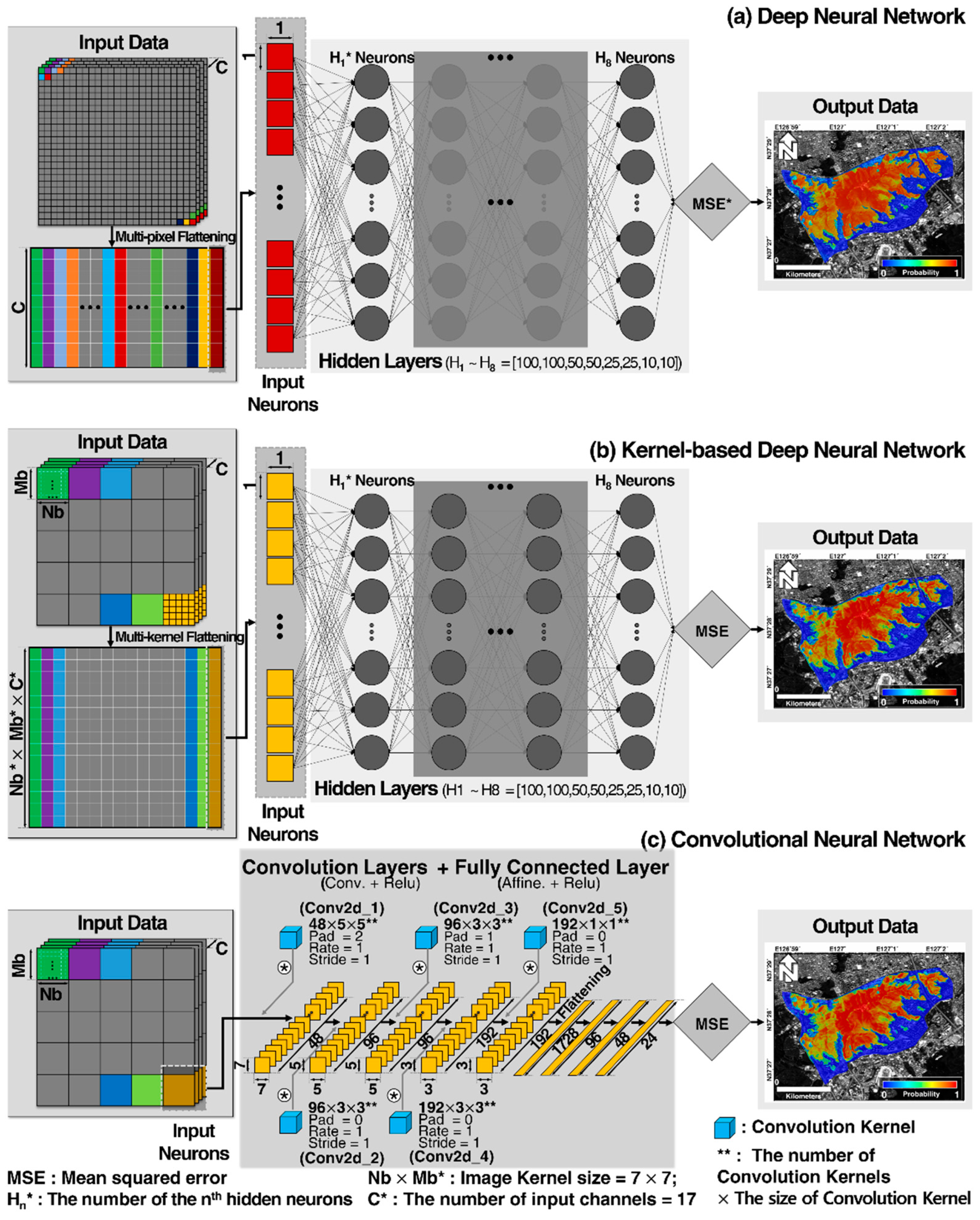
3.1. Deep Neural Network and Kernel-Based Deep Neural Network

ANNs are one of the most popular ML methods for prediction and classification across various fields. ANNs are composed of an input layer, a hidden layer, and an output layer; the input layer has as many input variables as the number of input variables in the model, and the output layer represents the prediction result. All layers between the input and output layers are referred to as hidden layers, and the number of hidden layers is determined through an empirical process [73]. The backpropagation algorithm is known to be the commonly used, effective method for training weight determination. Through the backpropagation algorithm, training is performed repeatedly, until a predefined error value is reached and finally is applied to predict for all the data by using the trained model [74].
DL methodology is an ML method based on this ANN, and it performs prediction and classification in the same way. Like the term “deep layer”, learning is performed by transforming data levels into different levels in DL methodology [75]. Recent ML studies have proposed various DL architectures (e.g., autoencoders, Restricted Boltzmann Machine (RBM), CNN, and Recurrent Neural Network (RNN)) [76]. In this study, a DNN and kernel-based DNN were applied and compared; the DNN can be interpreted as a deep version of an ANN. As the number of layers increases, the network becomes more complex, and the most appropriate layer for data can be created.
Specifically, in the case of a DNN using a stochastic gradient descent (SGD) in this study, the architecture was constructed using 100, 100, 50, 50, 25, 25, 10, 10 sequential hidden nodes, as shown in Figure 5 and Table 2. The rectified linear unit (ReLU) was selected as the activation function, and the nonlinear properties of the network were improved through the ReLU activation function [77]. The loss function was designated as the mean squared error (MSE), and the max epochs was set to 300 (Table 1). The batch size and learning rate were set to 150.00 and 0.01, respectively. In the process of calculating the weight for each node during training, the influence of the node becomes too high when the weight of a certain node is high. For example, only the neuron that has the most influence among the input neurons is reflected, and the result may appear as if it was created only by that layer. Therefore, the weight decay was used, which is a concept that prevents the weight of all nodes from becoming larger than necessary. By increasing the weight decay, we kept the overall weight low and used the conditions for all input neurons. Increasing the weight decay keeps the overall weight low and uses the conditions for all input neurons. The weight decay of DNN was set to 0.015 in this study. For a comparison of the results, the DNN and kernel-based DNN were set to the same parameters. The image kernel size was set to only 7 × 7 in the case of kernel-based DNN, as shown in the structure from Figure 5b.

3.2. Convolutional Neural Network

Recently, CNN applications for classification and prediction in various fields are increasing [78]. As mentioned above, CNNs are one of the well-known DL methodologies that show strong performance in image processing fields based on an ANN [79]. Important features of raw data can be automatically extracted through CNN [80]. Researchers have developed various structures depending on the type or purpose of the data; the basic architecture consists of an input layer, multiple hidden layers, and an output layer. The difference between CNNs and simple neural networks is that the hidden layer is composed of one or more convolutional and pooling layers, which share weights with multiple layers, pooling, and local connections [40]. The convolution layer, composed of several convolution kernels, repeatedly extracts features of the original data. The pooling layer prevents overfitting by reducing the dimension of the feature map through downsampling after the convolutional layer. In addition, it has an advantage of fast processing speed by greatly reducing the number of parameters by interpreting the input data as an image.
The CNN architecture in this study also consists of a convolution layer that learns convolution, and a pooling layer that improves computation performance by controlling overfitting and reducing the number of structures due to convolution through stable transformation [81]. In particular, the sizes of the convolutional kernel and the pooling kernel determine the scale of the convolution and pooling operations, respectively [82]. The activation function converts a linear relationship into a nonlinear relationship [83], and the optimizer iteratively updates the parameters at various learning rates. The loss function updates the weight by measuring the error between the predicted and actual values. In this study, the hyperparameter setting, a key step in building CNN architecture, is as follows in Table 1.
In this study, ReLU was selected as an activation function to improve the nonlinear property of the network; hereby, landslide susceptibility with a value between 0 and 1 is finally calculated. Stochastic gradient descent (SGD) was used as the optimizer, and MSE was selected as the loss function. The max epochs, batch size, and learning rate were set to 300.00, 150.00, and 0.01, respectively. Like DNN, the weight decay was set to 0.03, so that the weights of all input neurons were reflected, and stable loss and accuracy could be calculated. Image kernel size was set to 7 × 7 in the same way as kernel-based DNN. The feature map extracted through the convolution and pooling layers was reconstructed by the connection layer, and a classification result was derived through a nonlinear activation function. Figure 5 shows the prediction process using the CNN classifier used in this study.

3.3. Susceptibility Modeling and Mapping

For landslide susceptibility modeling and mapping using DNN, Kernel-based DNN and CNN models, a landslide training dataset was first constructed based on landslide occurrence locations selected from the research area. Since the study area is a small mountain located in the downtown area, the oversampling step was performed, considering that the number of landslide locations was only 103. The same number of samples where a non-landslide would occur was extracted as the landslide location samples, by random sampling with a slope of less than 5 degrees. After that, the sample was randomly divided into two sections: 80% was allocated to the training set, and the remaining 20% was extracted separately to use for performance evaluation [84,85,86]. The training set and the test set were adjusted through oversampling, which randomly adjusts the number of data by extracting the same data several times from imbalanced data. Finally, a total 20,000 of training (16,000) and test (4000) datasets were extracted and used for modeling.
The influential landslide variables were resampled in a grid format with 5 m spatial resolution. The value of each variable was extracted by overlaying 17 landslide influential variables on the training dataset, consisting of landslide and non-landslide samples. Finally, after training the model, susceptibility modeling was performed by applying it to the entire study area. Then, the results of landslide susceptibility were visually mapped with values from 0 to 1 from the three models.

3.4. Performance Evaluation of the Models

Model performance evaluation was performed to measure the predictive ability of the landslide model and whether it was suitable for the region. In this study, in order to evaluate the error of the prediction result, root mean square errors (RMSEs) were calculated for the prediction result of each model and the actual landslide information [85,87]. RMSEs were calculated using the 20% landslide locations that were stored for testing in the previous step.
Additionally, the accuracy of the model was calculated by calculating the area under the curve (AUC) of the precision–recall (PR) curve [88]. The PR curve is a curve with recall on the x-axis and precision on the y-axis, and is a line connecting recall and precision values for each data while varying the threshold value based on the susceptibility value of the model result. The AUC value created from the landslide modeling result depends on the recall and precision index of the x-axis and y-axis of the curve, respectively [88]. The AUC of the PR curve can be expressed as an average precision (AP) score, and it is the area of the graph when the PR curve is drawn. The AUC value approaches 1 when both recall and precision converge to the highest level, showing the model ability to efficiently predict the susceptibility of a landslide: the higher the value of the AUC of the PR, the higher the predictive ability of the model.

4. Results and Discussion

4.1. Susceptibility Maps

Figure 6 shows the three landslide susceptibility maps, derived from the model proposed in this study. Each map represents the susceptibility of landslide occurrence in the study area, derived through the DNN, kernel-based DNN, and CNN models, as described in the previous step. Due to the small study area, most areas can be classified into the same class when the map is graded. Therefore, the research area is represented by the susceptibility of occurrence from 0 to 1, and continuous susceptibility can be confirmed. The three models generally showed similar spatial distribution.
The proportions with susceptibility of less than 0.2 were 38.55%, 39.04%, and 38.30% in DNN, kernel-based DNN, and CNN models, respectively. On the other hand, the ratios of 0.8 or higher with a high susceptibility of landslide occurrence were 39.59%, 33.13%, and 34.47%, respectively. Relatedly, the DNN model shows a large number of regions with higher susceptibility, and in the case of kernel-based DNN, the resolution is slightly lowered. This is because the smoothing effect appeared as a result of using the kernel. Areas with high susceptibility of landslides were identified mainly along the north and south sides, where large debris flows occurred.
Since the slopes of Mt. Umyeon consists of gneiss, the forces remaining in the weathered gneiss layer after a torrential downpour reduce the amount of surface runoff and absorb a large amount of moisture into the weathered layer. Moisture in the saturated weathering layer reduces the resistance to bedrock, facilitating the downslope movement by gravity. As the resistance was sharply decreased, the physical erosion power was strengthened by the increase of the surface water flow, which erodes and mobilizes the mud and rocks. In kernel-based DNN and CNN, the effect on not only a single pixel but also neighboring pixels is considered at the same time, thus reflecting this phenomenon more realistically. In Figure 6, the probability of landslide is low in the mountain ridge in all models, and the valley slope forms a steep slope by lateral erosion.

4.2. Evaluation Results

The modeling process using the training dataset defined the relationship between landslide influencing variables with the location of the past landslides and future landslides, and the results were evaluated through AP scores with PR curves and statistical indicators of RMSE. The AP score curve showed that the performance of the DNN, kernel-based DNN, and CNN models was 99.45%, 99.44%, and 99.41%, respectively (Figure 7d–f). All showed over 99%, indicating that each model has very good accuracy in predicting landslides. RMSE was calculated based on the test dataset for the predictive model (Figure 7a–c). There were highest (0.1806) and lowest (0.1694) RMSEs for the DNN and kernel-based DNN models, respectively, and the CNN model had an RMSE of 0.1747. A low RMSE indicates good predictive power of the developed model. All three models show similar values, but the kernel-based DNN and CNN models were slightly better than the DNN model. This is obviously because the models are based on the kernel approach. However, the benefits of kernel processing were not significant in this study, because (1) the spatial resolutions of the forest and soil maps are low, and (2) the topographic relationships between adjacent pixels are given by the input data, such as TWI, SPI, SLF, etc. We can find one more difference between the DNN and the kernel-based models in Figure 6a–c. The kernel-based models shown in Figure 6b,c are smoothed due to the kernel calculation.
The AP scores were almost identical in all models, indicating that the model used in this study was reasonably accurate in mapping the susceptibility of landslides in the study area. The DNN showed the highest accuracy among three models, but the difference compared to the kernel-based DNN was very small, and the RMSE was relatively high. As a result of using an additional kernel, the RMSE value decreased by about 6.2%, and such inconsistency did not occur. Therefore, it can be interpreted that the kernel-based DNN model exhibits better performance for predicting future landslides than the DNN model. In addition, the weight decay was increased to adjust the total weight, in order to prevent the weight of a specific node from being higher than necessary, thereby preventing the result of being weighted by a specific variable. By preventing overestimation, it was possible to prevent the results from being greatly affected by the slightly adjusted training data. Through this, the results of improving the precision of the test data, as well as the precision of the training data, were confirmed. The three results compared in this study all showed similar patterns due to the limited input neurons, and it is difficult to specify which model is better. However, reliable results were obtained in all of the DNN, kernel-based DNN, and CNN models, and can be applied not only to landslides, but also to modeling the susceptibility of natural phenomena and various regions, such as flood and forest fire mapping.

5. Conclusions

In the present study, a methodological approach was introduced to develop a DNN model, a kernel-based DNN that combines a kernel with the DNN model, and a CNN model, all of which were trained based on a SGD. The location data for training the susceptibility of a landslide was constructed by analyzing aerial photographs and field survey results. Topographic variables were extracted from aerial photographs and digital topographic maps, and soil and forest influencing variables were also extracted. A landslide inventory was constructed using the training dataset built through oversampling for the landslide area and non-landslide area, with the landslide influencing variables; modeling was performed for three models based on the inventory. Finally, the resulting map was evaluated using a test set (20%) of landslide data that was not used for training. The training and prediction functions of the developed DL model were evaluated and compared with the results of RMSE estimation and AP score analysis. The experimental results showed that the optimized DNN model had the highest predictive power (99.45%), followed by the kernel-based DNN (99.44%) and CNN model (99.41%) methods. The recall and precision of all models showed sufficiently high results, and the performance of all models was more than 99% satisfactory.
The expected landslide susceptibility was high near the top of the mountain and was similar to the existing landslide pattern. The susceptibility of landslides decreases according to the slope of the susceptibility map of this study, which is a logical result of the occurrence of debris flow due to the shape of the topography. Nevertheless, there are some limitations to the implementation of neural network (NN)-based DL models. In selecting variables, it is necessary to apply a different methodology in advance, in order to understand the fundamental relationship between variables and landslides, just as variables were selected based on previous studies in this study. Also, the model architecture is less intuitive due to the black box of the NN model. That means selecting the right hyperparameters is a task that requires experiential expertise.
Compared to water-related disasters, landslides were not previously considered a serious problem in urban areas. Most cities developed rapidly without taking into account the damage caused by natural disasters in the process of urbanization. However, due to the recent increase in local heavy rain, extreme precipitation and population pressure in any part of the city can have serious consequences. Therefore, it is important to establish basic scientific data to prevent landslides in urban areas such as Seoul. Regarding the applicability of the developed methodology, the results of this study are expected to support decision-making to identify spatial problems related to urban landslides and effective risk reduction policies.

Author Contributions

S.L. (Sunmin Lee), W.-K.B., and S.L. (Saro Lee) collected data. W.-K.B. and H.-S.J. processed input data. S.L. (Sunmin Lee) and H.-S.J. managed the paperwork and interpreted the results. H.-S.J. suggested the idea and prepared the data. All of the authors contributed to the writing of each part. All authors have read and agreed to the published version of the manuscript.

Funding

This work was supported by the National Research Foundation of Korea, funded by the Korean government under grant NRF-2018M1A3A3A02066008. This research was supported by the Basic Research Project of the Korea Institute of Geoscience and Mineral Resources (KIGAM) and Project of Environmental Business Big Data Platform and Center Construction funded by the Ministry of Science and ICT. This research was supported by a grant (20010017) of R&D Program of Responding Technology to Climate Disaster such as Heat Wave funded by Ministry of Interior and Safety (MOIS, Korea) which was conducted by the Korea Environment Institute (KEI).

Conflicts of Interest

The authors declare no conflict of interest.

References

  1. Landslide Information System. Available online: http://sansatai.forest.go.kr/ (accessed on 26 September 2020).
  2. Kang, S.; Lee, S.; Nikhil, N.; Park, J.-Y. Analysis of Differences in Geomorphological Characteristics on Initiation of Landslides and Debris Flows. J. Korean Soc. Hazard Mitig. 2015, 15, 249–258. [Google Scholar] [CrossRef] [Green Version]
  3. Lee, J. Management system for landslides hazard area using GIS. J. Korea Soc. For. Eng. Technol. 2005, 3, 245–255. [Google Scholar]
  4. Lee, H.-G.; Kim, G.-H. Landslide Risk Assessment in Inje Using Logistic Regression Model. J. Korean Soc. Surv. Geodesy Photogramm. Cartogr. 2012, 30, 313–321. [Google Scholar]
  5. Kim, G. A Basic Study on the Development of the Guidelines on Setting Debris Flow Hazards; Research Institute for Gangwon: Chuncheon-s, Korea, 2011; p. 170. [Google Scholar]
  6. Vagnon, F.; Ferrero, A.M.; Pirulli, M.; Segalini, A. Theoretical and experimental study for the optimization of flexible barriers to restrain debris flows. Geam. Environ. Min. Geo. Eng. 2015, 149, 29–35. [Google Scholar]
  7. Vagnon, F.; Ferrero, A.M.; Alejano, L.R. Reliability-based design for debris flow barriers. Landslides 2019, 17, 49–59. [Google Scholar] [CrossRef]
  8. Vagnon, F. Design of active debris flow mitigation measures: A comprehensive analysis of existing impact models. Landslides 2020, 17, 313–333. [Google Scholar] [CrossRef]
  9. Miyamoto, K. Two dimensional numerical simulation of landslide mass movement. J. Eros. Control Eng. 2002, 55, 5–13. [Google Scholar]
  10. Pellegrino, A.M.; Schippa, L. Macro viscous regime of natural dense granular mixtures. Int. J. Geomate 2013, 4, 482–489. [Google Scholar] [CrossRef]
  11. Schippa, L. Modeling the effect of sediment concentration on the flow-like behavior of natural debris flow. Int. J. Sediment Res. 2020, 35, 315–327. [Google Scholar] [CrossRef]
  12. Pellegrino, A.M.; Schippa, L. A laboratory experience on the effect of grains concentration and coarse sediment on the rheology of natural debris-flows. Environ. Earth Sci. 2018, 77, 749. [Google Scholar] [CrossRef]
  13. Kim, P. Numerical modeling for the detection and movement of debris flow using detailed soil maps and GIS. J. Korean Soci. Civ. Eng. 2017. [Google Scholar] [CrossRef] [Green Version]
  14. VanDine, D. Debris Flow Control Structures for Forest Engineering; Working paper; Ministry of Forests: Victoria, BC, Canada, 1996.
  15. Lee, S.; Lee, M.-J.; Won, J.-S. Study on Landslide using GIS and Remote Sensing at the Kangneung Area (II)-Landslide Susceptibility Mapping and Cross-Validation using the Probability Technique. Econ. Environ. Geol. 2004, 37, 521–532. [Google Scholar]
  16. Kose, D.D.; Turk, T. GIS-based fully automatic landslide susceptibility analysis by weight-of-evidence and frequency ratio methods. Phys. Geogr. 2019, 40, 481–501. [Google Scholar] [CrossRef]
  17. Yan, F.; Zhang, Q.; Ye, S.; Ren, B. A novel hybrid approach for landslide susceptibility mapping integrating analytical hierarchy process and normalized frequency ratio methods with the cloud model. Geomorphology 2019, 327, 170–187. [Google Scholar] [CrossRef]
  18. Zhang, Y.-X.; Lan, H.-X.; Li, L.-P.; Wu, Y.-M.; Chen, J.-H.; Tian, N.-M. Optimizing the frequency ratio method for landslide susceptibility assessment: A case study of the Caiyuan Basin in the southeast mountainous area of China. J. Mt. Sci. 2020, 17, 340–357. [Google Scholar] [CrossRef]
  19. Feby, B.; Achu, A.; Jimnisha, K.; Ayisha, V.; Reghunath, R. Landslide susceptibility modelling using integrated evidential belief function based logistic regression method: A study from Southern Western Ghats, India. Remote Sens. Appl. Soc. Environ. 2020, 20, 100411. [Google Scholar] [CrossRef]
  20. Nhu, V.-H.; Shirzadi, A.; Shahabi, H.; Singh, S.K.; Al-Ansari, N.; Clague, J.J.; Jaafari, A.; Chen, W.; Miraki, S.; Dou, J. Shallow Landslide Susceptibility Mapping: A Comparison between Logistic Model Tree, Logistic Regression, Naïve Bayes Tree, Artificial Neural Network, and Support Vector Machine Algorithms. Int. J. Environ. Res. Public Health 2020, 17, 2749. [Google Scholar] [CrossRef]
  21. Soma, A.S.; Kubota, T.; Mizuno, H. Optimization of causative factors using logistic regression and artificial neural network models for landslide susceptibility assessment in Ujung Loe Watershed, South Sulawesi Indonesia. J. Mt. Sci. 2019, 16, 383–401. [Google Scholar] [CrossRef]
  22. Abedini, M.; Ghasemian, B.; Shirzadi, A.; Bui, D.T. A comparative study of support vector machine and logistic model tree classifiers for shallow landslide susceptibility modeling. Environ. Earth Sci. 2019, 78, 560. [Google Scholar]
  23. Saha, A.; Saha, S. Comparing the efficiency of weight of evidence, support vector machine and their ensemble approaches in landslide susceptibility modelling: A study on Kurseong region of Darjeeling Himalaya, India. Remote Sens. Appl. Soc. Environ. 2020, 19, 100323. [Google Scholar]
  24. Moayedi, H.; Mehrabi, M.; Mosallanezhad, M.; Rashid, A.S.A.; Pradhan, B. Modification of landslide susceptibility mapping using optimized PSO-ANN technique. Eng. Comput. 2019, 35, 967–984. [Google Scholar] [CrossRef]
  25. Sevgen, E.; Kocaman, S.; Nefeslioglu, H.A.; Gokceoglu, C. A novel performance assessment approach using photogrammetric techniques for landslide susceptibility mapping with logistic regression, ANN and random forest. Sensors 2019, 19, 3940. [Google Scholar] [CrossRef] [PubMed] [Green Version]
  26. Yu, C.; Chen, J. Landslide Susceptibility Mapping Using the Slope Unit for Southeastern Helong City, Jilin Province, China: A Comparison of ANN and SVM. Symmetry 2020, 12, 1047. [Google Scholar] [CrossRef]
  27. Arabameri, A.; Pradhan, B.; Rezaei, K.; Lee, S.; Sohrabi, M. An ensemble model for landslide susceptibility mapping in a forested area. Geocarto Int. 2019, 35, 1680–1705. [Google Scholar] [CrossRef]
  28. Sachdeva, S.; Bhatia, T.; Verma, A.K. A novel voting ensemble model for spatial prediction of landslides using GIS. Int. J. Remote Sens. 2020, 41, 929–952. [Google Scholar] [CrossRef]
  29. Thai Pham, B.; Shirzadi, A.; Shahabi, H.; Omidvar, E.; Singh, S.K.; Sahana, M.; Talebpour Asl, D.; Bin Ahmad, B.; Kim Quoc, N.; Lee, S. Landslide susceptibility assessment by novel hybrid machine learning algorithms. Sustainability 2019, 11, 4386. [Google Scholar] [CrossRef] [Green Version]
  30. Zhang, T.-Y.; Han, L.; Zhang, H.; Zhao, Y.-H.; Li, X.-A.; Zhao, L. GIS-based landslide susceptibility mapping using hybrid integration approaches of fractal dimension with index of entropy and support vector machine. J. Mt. Sci. 2019, 16, 1275–1288. [Google Scholar] [CrossRef]
  31. Jaafari, A.; Panahi, M.; Pham, B.T.; Shahabi, H.; Bui, D.T.; Rezaie, F.; Lee, S. Meta optimization of an adaptive neuro-fuzzy inference system with grey wolf optimizer and biogeography-based optimization algorithms for spatial prediction of landslide susceptibility. Catena 2019, 175, 430–445. [Google Scholar] [CrossRef]
  32. Mehrabi, M.; Pradhan, B.; Moayedi, H.; Alamri, A. Optimizing an Adaptive Neuro-Fuzzy Inference System for Spatial Prediction of Landslide Susceptibility Using Four State-of-the-art Metaheuristic Techniques. Sensors 2020, 20, 1723. [Google Scholar] [CrossRef] [Green Version]
  33. Moayedi, H.; Mehrabi, M.; Kalantar, B.; Mu’Azu, M.A.; Rashid, A.S.A.; Foong, L.K.; Nguyen, H. Novel hybrids of adaptive neuro-fuzzy inference system (ANFIS) with several metaheuristic algorithms for spatial susceptibility assessment of seismic-induced landslide. Geomat. Nat. Hazards Risk 2019, 10, 1879–1911. [Google Scholar] [CrossRef] [Green Version]
  34. Panahi, M.; Gayen, A.; Pourghasemi, H.R.; Rezaie, F.; Lee, S. Spatial prediction of landslide susceptibility using hybrid support vector regression (SVR) and the adaptive neuro-fuzzy inference system (ANFIS) with various metaheuristic algorithms. Sci. Total. Environ. 2020, 741, 139937. [Google Scholar] [CrossRef] [PubMed]
  35. Arabameri, A.; Pradhan, B.; Rezaei, K.; Sohrabi, M.; Kalantari, Z. GIS-based landslide susceptibility mapping using numerical risk factor bivariate model and its ensemble with linear multivariate regression and boosted regression tree algorithms. J. Mt. Sci. 2019, 16, 595–618. [Google Scholar] [CrossRef]
  36. Lee, S. Current and future status of GIS-based landslide susceptibility mapping: A literature review. Korean J. Remote Sens. 2019, 35, 179–193. [Google Scholar]
  37. Schmidhuber, J. Deep Learning: Our Miraculous Year 1990–1991. arXiv 2020, arXiv:2005.05744. [Google Scholar]
  38. Qi, C.; Fourie, A.; Ma, G.; Tang, X. A hybrid method for improved stability prediction in construction projects: A case study of stope hangingwall stability. Appl. Soft Comput. 2018, 71, 649–658. [Google Scholar] [CrossRef]
  39. Can, A.; Dagdelenler, G.; Ercanoglu, M.; Sonmez, H. Landslide susceptibility mapping at Ovacık-Karabük (Turkey) using different artificial neural network models: Comparison of training algorithms. Bull. Eng. Geol. Environ. 2019, 78, 89–102. [Google Scholar] [CrossRef]
  40. Ghorbanzadeh, O.; Blaschke, T.; Gholamnia, K.; Meena, S.R.; Tiede, D.; Aryal, J. Evaluation of different machine learning methods and deep-learning convolutional neural networks for landslide detection. Remote Sens. 2019, 11, 196. [Google Scholar] [CrossRef] [Green Version]
  41. Ghorbanzadeh, O.; Meena, S.R.; Blaschke, T.; Aryal, J. UAV-based slope failure detection using deep-learning convolutional neural networks. Remote Sens. 2019, 11, 2046. [Google Scholar] [CrossRef] [Green Version]
  42. Mohan, A.; Singh, A.K.; Kumar, B.; Dwivedi, R. Review on remote sensing methods for landslide detection using machine and deep learning. Trans. Emerg. Telecommun. Technol. 2020, e3998. [Google Scholar] [CrossRef]
  43. Wang, Y.; Fang, Z.; Hong, H. Comparison of convolutional neural networks for landslide susceptibility mapping in Yanshan County, China. Sci. Total Environ. 2019, 666, 975–993. [Google Scholar] [CrossRef]
  44. Aghdam, I.N.; Varzandeh, M.H.M.; Pradhan, B. Landslide susceptibility mapping using an ensemble statistical index (Wi) and adaptive neuro-fuzzy inference system (ANFIS) model at Alborz Mountains (Iran). Environ. Earth Sci. 2016, 75, 1–20. [Google Scholar] [CrossRef]
  45. Li, Y.; Chen, W. Landslide susceptibility evaluation using hybrid integration of evidential belief function and machine learning techniques. Water 2020, 12, 113. [Google Scholar] [CrossRef] [Green Version]
  46. Lee, S.; Lee, M.-J.; Jung, H.-S. Data mining approaches for landslide susceptibility mapping in Umyeonsan, Seoul, South Korea. Appl. Sci. 2017, 7, 683. [Google Scholar] [CrossRef] [Green Version]
  47. Yune, C.-Y.; Chae, Y.-K.; Paik, J.; Kim, G.; Lee, S.-W.; Seo, H.-S. Debris flow in metropolitan area—2011 Seoul debris flow. J. Mt. Sci. 2013, 10, 199–206. [Google Scholar] [CrossRef]
  48. Jun, K.; Oh, C.; Jun, B. Study on analyzing characteristics which causes a debris flow–focusing on the relation with slope and river. J. Saf. Crisis Manag. 2011, 7, 223–232. [Google Scholar]
  49. Pradhan, A.M.S.; Kim, Y.-T. Spatial data analysis and application of evidential belief functions to shallow landslide susceptibility mapping at Mt. Umyeon, Seoul, Korea. Bull. Eng. Geol. Environ. 2017, 76, 1263–1279. [Google Scholar] [CrossRef]
  50. Kim, S.; Paik, J.; Kim, K.S. Run-out modeling of debris flows in Mt. Umyeon using FLO-2D. J. Korean Soc. Civ. Eng. 2013, 33, 965–974. [Google Scholar] [CrossRef] [Green Version]
  51. Ko, S.M.; Lee, S.W.; Yune, C.-Y.; Kim, G. Topographic analysis of landslides in Umyeonsan. J. Korean Soc. Surv. Geod. Photogramm. Cartogr. 2014, 32, 55–62. [Google Scholar] [CrossRef]
  52. Lee, M.-J.; Park, I.; Lee, S. Forecasting and validation of landslide susceptibility using an integration of frequency ratio and neuro-fuzzy models: A case study of Seorak mountain area in Korea. Environ. Earth Sci. 2015, 74, 413–429. [Google Scholar] [CrossRef]
  53. Park, S.-J.; Lee, C.-W.; Lee, S.; Lee, M.-J. Landslide susceptibility mapping and comparison using decision tree models: A Case Study of Jumunjin Area, Korea. Remote Sens. 2018, 10, 1545. [Google Scholar] [CrossRef] [Green Version]
  54. KIM, J.-H.; OH, J.-S. A Study on the Geological Characteristics and Slope Landform Changes of Mt. Umyeon. Korean J. Nat. Conserv. 2013, 11, 1–14. [Google Scholar] [CrossRef]
  55. Dehnavi, A.; Aghdam, I.N.; Pradhan, B.; Varzandeh, M.H.M. A new hybrid model using step-wise weight assessment ratio analysis (SWARA) technique and adaptive neuro-fuzzy inference system (ANFIS) for regional landslide hazard assessment in Iran. Catena 2015, 135, 122–148. [Google Scholar] [CrossRef]
  56. Seoul City. Supplemental investigation report of causes of Umyeonsan landslides. Seoul: Seoul City 2014. [Google Scholar]
  57. Capitani, M.; Ribolini, A.; Bini, M. The slope aspect: A predisposing factor for landsliding? Comptes Rendus Geosci. 2013, 345, 427–438. [Google Scholar] [CrossRef]
  58. Pourghasemi, H.R.; Yansari, Z.T.; Panagos, P.; Pradhan, B. Analysis and evaluation of landslide susceptibility: A review on articles published during 2005–2016 (periods of 2005–2012 and 2013–2016). Arab. J. Geosci. 2018, 11, 193. [Google Scholar] [CrossRef]
  59. Conrad, O.; Bechtel, B.; Bock, M.; Dietrich, H.; Fischer, E.; Gerlitz, L.; Wehberg, J.; Wichmann, V.; Böhner, J. System for automated geoscientific analyses (SAGA) v. 2.1. 4. Geosci. Model Dev. Discuss. 2015, 8. [Google Scholar] [CrossRef] [Green Version]
  60. Oh, H.-J.; Pradhan, B. Application of a neuro-fuzzy model to landslide-susceptibility mapping for shallow landslides in a tropical hilly area. Comput. Geosci. 2011, 37, 1264–1276. [Google Scholar] [CrossRef]
  61. Moore, I.D.; Grayson, R.; Ladson, A. Digital terrain modelling: A review of hydrological, geomorphological, and biological applications. Hydrol. Process. 1991, 5, 3–30. [Google Scholar] [CrossRef]
  62. Wilson, J.P.; Gallant, J.C. Terrain Analysis: Principles and Applications; John Wiley & Sons: Hoboken, NJ, USA, 2000. [Google Scholar]
  63. Conoscenti, C.; Di Maggio, C.; Rotigliano, E. GIS analysis to assess landslide susceptibility in a fluvial basin of NW Sicily (Italy). Geomorphology 2008, 94, 325–339. [Google Scholar] [CrossRef]
  64. Nefeslioglu, H.A.; Gokceoglu, C.; Sonmez, H. An assessment on the use of logistic regression and artificial neural networks with different sampling strategies for the preparation of landslide susceptibility maps. Eng. Geol. 2008, 97, 171–191. [Google Scholar] [CrossRef]
  65. Wischmeier, W.H.; Smith, D.D. Predicting Rainfall Erosion Losses: A Guide to Conservation Planning; United States Department of Agriculture, Science and Education Administration: Beltsville, MD, USA, 1978.
  66. Böhner, J.; Selige, T. Spatial prediction of soil attributes using terrain analysis and climate regionalisation. In SAGA—Analyses and Modelling Applications; Goltze: Göttingen, Germany, 2006. [Google Scholar]
  67. Nguyen, V.V.; Pham, B.T.; Vu, B.T.; Prakash, I.; Jha, S.; Shahabi, H.; Shirzadi, A.; Ba, D.N.; Kumar, R.; Chatterjee, J.M. Hybrid machine learning approaches for landslide susceptibility modeling. Forests 2019, 10, 157. [Google Scholar] [CrossRef] [Green Version]
  68. Hjerdt, K.; McDonnell, J.; Seibert, J.; Rodhe, A. A new topographic index to quantify downslope controls on local drainage. Water Resour. Res. 2004, 40. [Google Scholar] [CrossRef] [Green Version]
  69. Ohlmacher, G.C.; Davis, J.C. Using multiple logistic regression and GIS technology to predict landslide hazard in northeast Kansas, USA. Eng. Geol. 2003, 69, 331–343. [Google Scholar] [CrossRef]
  70. Van Westen, C.; Van Asch, T.W.; Soeters, R. Landslide hazard and risk zonation—why is it still so difficult? Bull. Eng. Geol. Environ. 2006, 65, 167–184. [Google Scholar] [CrossRef]
  71. Mogaji, K.A.; San Lim, H.; Abdullah, K. Modeling of groundwater recharge using a multiple linear regression (MLR) recharge model developed from geophysical parameters: A case of groundwater resources management. Environ. Earth Sci. 2015, 73, 1217–1230. [Google Scholar] [CrossRef]
  72. JONES, H.G. Estimation of an effective soil water potential at the root surface of transpiring plants. Plant Cell Environ. 1983, 6, 671–674. [Google Scholar]
  73. Du, S.S.; Wang, Y.; Zhai, X.; Balakrishnan, S.; Salakhutdinov, R.R.; Singh, A. How many samples are needed to estimate a convolutional neural network? In Proceedings of the Advances in Neural Information Processing Systems 31 (NeurIPS 2018), Montreal, QC, Canada, 2–8 December 2018; pp. 373–383. [Google Scholar]
  74. Liu, W.; Wang, Z.; Liu, X.; Zeng, N.; Liu, Y.; Alsaadi, F.E. A survey of deep neural network architectures and their applications. Neurocomputing 2017, 234, 11–26. [Google Scholar] [CrossRef]
  75. Patterson, J.; Gibson, A. Deep Learning: A practitioner’s Approach; O‘Reilly Media Inc.: Boston, MA, USA, 2017. [Google Scholar]
  76. Alom, M.Z.; Taha, T.M.; Yakopcic, C.; Westberg, S.; Sidike, P.; Nasrin, M.S.; Hasan, M.; Van Essen, B.C.; Awwal, A.A.; Asari, V.K. A state-of-the-art survey on deep learning theory and architectures. Electronics 2019, 8, 292. [Google Scholar] [CrossRef] [Green Version]
  77. Agarap, A.F. Deep learning using rectified linear units (relu). arXiv 2018, arXiv:1803.08375. [Google Scholar]
  78. Zuo, R.; Xiong, Y.; Wang, J.; Carranza, E.J.M. Deep learning and its application in geochemical mapping. Earth-Sci. Rev. 2019, 192, 1–14. [Google Scholar] [CrossRef]
  79. LeCun, Y.; Bengio, Y.; Hinton, G. Deep learning. Nature 2015, 521, 436–444. [Google Scholar] [CrossRef] [PubMed]
  80. Lawrence, S.; Giles, C.L.; Tsoi, A.C.; Back, A.D. Face recognition: A convolutional neural-network approach. IEEE Trans. Neural Netw. 1997, 8, 98–113. [Google Scholar] [CrossRef] [Green Version]
  81. Nair, V.; Hinton, G.E. Rectified linear units improve restricted boltzmann machines. In Proceedings of the 27th International Conference on Machine Learning, Haifa, Israel, 21–24 June 2010. [Google Scholar]
  82. Golik, P.; Tüske, Z.; Schlüter, R.; Ney, H. Convolutional neural networks for acoustic modeling of raw time signal in LVCSR. In Proceedings of the 16th Annual Conference of the International Speech Communication Association, Dresden, Germany, 6–10 September 2015. [Google Scholar]
  83. Audebert, N.; Le Saux, B.; Lefèvre, S. Deep learning for classification of hyperspectral data: A comparative review. IEEE Geosci. Remote Sens. Mag. 2019, 7, 159–173. [Google Scholar] [CrossRef] [Green Version]
  84. Pradhan, B.; Lee, S. Landslide susceptibility assessment and factor effect analysis: Backpropagation artificial neural networks and their comparison with frequency ratio and bivariate logistic regression modelling. Environ. Model. Softw. 2010, 25, 747–759. [Google Scholar] [CrossRef]
  85. Tien Bui, D.; Shahabi, H.; Shirzadi, A.; Chapi, K.; Alizadeh, M.; Chen, W.; Mohammadi, A.; Ahmad, B.B.; Panahi, M.; Hong, H. Landslide detection and susceptibility mapping by airsar data using support vector machine and index of entropy models in cameron highlands, malaysia. Remote Sens. 2018, 10, 1527. [Google Scholar] [CrossRef] [Green Version]
  86. Mersha, T.; Meten, M. GIS-based landslide susceptibility mapping and assessment using bivariate statistical methods in Simada area, northwestern Ethiopia. Geoenviron. Disasters 2020, 7, 1–22. [Google Scholar] [CrossRef]
  87. Pham, B.T.; Prakash, I.; Singh, S.K.; Shirzadi, A.; Shahabi, H.; Bui, D.T. Landslide susceptibility modeling using Reduced Error Pruning Trees and different ensemble techniques: Hybrid machine learning approaches. Catena 2019, 175, 203–218. [Google Scholar] [CrossRef]
  88. Davis, J.; Goadrich, M. The relationship between Precision-Recall and ROC curves. In Proceedings of the 23rd International Conference on Machine Learning, Pittsburgh, PA, USA, 25–29 June 2006; pp. 233–240. [Google Scholar]
Figure 1. The study area of Mt. Umyeon.
Applsci 10 08189 g001
Figure 2. Landslide locations from aerial photographs after landslides in 2011: (a) Mt.Umyeon area after the landslides in 2011, (b) debris flows in northern part of Mt. Umyeon and (c) damage of residential areas including apartments.
Applsci 10 08189 g002
Figure 3. Topographical variables influencing landslides used in this study: (a) slope gradient, (b) slope aspect, (c) curvature, (d) topographic wetness index (TWI), (e) stream power index (SPI), (f) slope length factor (SLF), (g) standardized height, (h) valley depth, and (i) downslope distance gradient (DDG).
Applsci 10 08189 g003
Figure 4. Landslide-influencing variables related to vegetation and soil: (a) timber type, (b) timber diameter, (c) timber density, (d) timber age, (e) soil depth, (f) soil drainage, (g) soil topography, and (h) soil texture.
Applsci 10 08189 g004
Figure 5. Model architecture proposed in this study: (a) Deep Neural Network, (b) kernel-based Deep Neural Network, and (c) Convolutional Neural Network.
Applsci 10 08189 g005
Figure 6. Landslide susceptibility maps generated using deep learning models: Using a (a) deep neural network (DNN), (b) kernel-based DNN, NS (c) convolutional neural network (CNN) model.
Applsci 10 08189 g006
Figure 7. Model performance evaluation results: (ac) root mean square errors (RMSEs) and (df) average precision (AP) scores of the DNN, kernel-based DNN, and CNN models.
Applsci 10 08189 g007
Table 1. Landslide influential variables used in this study.
Original DataVariablesData TypeScale
Aerial photographLandslide locationPoint1:1000
Topographical map a Slope gradient [°]
Slope aspect
Curvature
Topographic wetness index (TWI)
Stream power index (SPI)
Slope length factor (SLF)
Standardized height (m)
Valley depth (m)
Downslope distance gradient (DDG) (rad)
Grid1:1000
Forest map bTimber diameter
Timber type
Timber density
Timber age
Polygon1:25,000
Soil map cSoil depth
Soil drainage
Soil topography
Soil texture
Polygon1:25,000
a The digital topographic map by the National Geographic Information Institute; b the forest map produced by the Korea Forest Service; c the soil map produced by Rural Development Administration.
Table 2. Model parameters used in this study.
Model ParametersDNNKDNNCNN
Input data dimension- 7 × 7 7 × 7
Filter depth in convolutional layers--[48, 96, 96, 192, 192]
Filter size in convolutional layers--[3, 3, 3, 3, 1]
Number of nodes in fully connected layer[100, 100, 50, 50, 25, 25, 10, 10][96, 48, 24]
Activation functionThe rectified linear unit (ReLU)
OptimizerStochastic gradient descent (SGD)
Loss functionMean squared error (MSE)
Max epochs300.00
Batch size150.00
Learning rate0.01
Weight decay0.0150.0150.030
Publisher’s Note: MDPI stays neutral with regard to jurisdictional claims in published maps and institutional affiliations.

