Improved Photoacoustic Imaging of Numerical Bone Model Based on Attention Block U-Net Deep Learning Network

Abstract

Photoacoustic (PA) imaging can provide both chemical and micro-architectural information for biological tissues. However, photoacoustic imaging for bone tissue remains a challenging topic due to complicated ultrasonic propagations in the porous bone. In this paper, we proposed a post-processing method based on the convolution neural network (CNN) to improve the image quality of PA bone imaging in a numerical model. To be more adaptive for imaging bone samples with complex structure, an attention block U-net (AB-U-Net) network was designed from the standard U-net by integrating the attention blocks in the feature extraction part. The k-wave toolbox was used for the simulation of photoacoustic wave fields, and then the direct reconstruction algorithm—time reversal was adopted for generating a dataset of deep learning. The performance of the proposed AB-U-Net network on the reconstruction of photoacoustic bone imaging was analyzed. The results show that the AB-U-Net based deep learning method can obtain the image presented as a clear bone micro-structure. Compared with the traditional photoacoustic reconstruction method, the AB-U-Net-based reconstruction algorithm can achieve better performance, which greatly improves image quality on test set with peak signal to noise ratio (PSNR) and structural similarity increased (SSIM) by 3.83 dB and 0.17, respectively. The deep learning method holds great potential in enhancing PA imaging technology for bone disease detection.

1. Introduction

In recent years, the high incidence of orthopedic diseases like osteoporosis (approximately 40% of women and 20% of men over the age of 50 years [1]), and the resulting high costs of the treatment make it increasingly essential to monitor bone quality [2]. Several techniques have been developed for bone assessment non-invasively. Dual-energy X-ray absorptiometry (DXA) is regarded as the gold standard for bone mineral density (BMD) measurement [3,4]. BMD measurement reflects the mineral content in bone tissue, but it can only explain about 60–70% of bone strength changes [5,6]. Other variances like trabecular micro-structure are reported to be important complements for bone evaluation [7]. Although computerized tomography (CT) can provide bone geometry with relatively high resolution, it is achieved at the cost of delivering a considerable radiation dose [8]. As a newly non-ionizing radiation modality, quantitative ultrasound (QUS) has the advantages of low cost, portability and accessibility [9,10]. The speed of sound (SOS) and broadband ultrasound attenuation (BUA) are two important parameters. They are measured as the mean values of the ultrasonically interrogated bone tissue, which are highly related to bone quantity, but rarely provide information about bone micro-structure [6]. The QUS parameters based on ultrasonic backscattering are used to characterize bone densities and structure [11,12,13,14,15,16]. Ultrasonic backscatter measurements could even reflect additional density and structural features unrelated to current BMD measurement [16,17]. Moreover, new advances in ultrasound imaging enable the visualization of bone anatomy [18].

Photoacoustic (PA) imaging is a newly emerging noninvasive imaging method based on different optical absorption in biological tissues [19,20,21,22]. It is based on optical excitation and ultrasonic detection. The acoustic waves are generated by irradiating a short pulse laser on biological tissue with thermoelastic expansion. Ultrasonic signals propagating through the tissue are recorded using ultrasonic transducers. With different reconstruction algorithms, the PA imaging is to restore initial pressure of the tissue from detected signals [23]. As an imaging mode with non-ionizing radiation, PA imaging poses no health hazard compared with other X-ray based imaging modalities. Combining the advantage of ultrasonically deep imaging depth and optically high contrast, PA imaging presents the spatial distribution of tissue with high image quality. It has played an important role in the clinical detection of tumors and vessels [24,25,26,27,28]. Recent studies also have investigated the possibility of PA technology in the application of measuring BMD, bone composition and structure [29,30,31,32]. Wang et al. demonstrated that the feasibility of PA imaging in human peripheral joints and the imaging depth is sufficient to penetrate through larger human joints [33]. Yang et al. achieved the detection of bone mineralization or decollagenization by combining PA and ultrasound imaging modalities [34]. Furthermore, the latest experiments by Merrill validated that the PA reconstructed image of ex vivo porcine bone is available through PA microscopy system [35]. For bone imaging, PA imaging shows its great potential and a promising prospect.

Despite exciting progress in PA imaging, the image reconstruction for bone tissue is still a big challenge. Unlike the soft tissue, bone tissue is a complex porous material composed by trabeculae bone and bone marrow filled within the pores [36]. The porous bone tissue is a strongly scattering medium with heavy ultrasonic attenuation and phase distortions, making it difficult to image bone structure with high PA image quality [37]. Besides, the high heterogeneity of bone tissue would produce large variations in ultrasonic velocity. There is a large difference in SOS between the two components of bone tissue, i.e., a typical SOS is 1500 m/s and 4000 m/s for bone marrow and trabeculae, respectively [38,39]. However, traditional PA imaging algorithms assume that the SOS is uniform in porous bone tissue, and this uniform assumption of SOS for bone tissue leads to calculation errors and a following distortion for reconstructed images [40]. In addition, due to the limitation of experimental conditions and time costs, the highly under-sampled data, which is caused by a sparse array of detector points, cannot meet the requirement of artifact-free imaging advised by Shannon’s sampling theory [41]. Approaches to the above problems have been discussed recently [42,43,44,45]. Wang et al. elaborated an iterative reconstruction method, estimating the velocity distribution to reduce the effects of acoustic heterogeneity, while the iterative method is implemented at the cost of a formidable computational burden [42]. A new method called ultrasonic transmission tomography (UTT) was proposed to correct acoustic speed variations. However, the UTT algorithm assumes that ultrasound pulses travel in straight lines through the target, it may be invalid to restore the tissue of great acoustic speed variations like bones [43]. Zhang et al. investigated a heuristic method for reconstructing weakly scattering object, but it is limited at a request of a complete set of PAT measurement data [44]. Rui et al. utilized a matrix filtering method, successfully recovering the PA image inside a skull-like scattering layer, however, it can hardly restore the information of bone micro-structure accurately [45].

Convolutional neural networks (CNN) are a type of deep feedforward neural network with convolution computation [46]. It is one of the representative algorithms of deep learning. Based on their rich representation power, fast inference and filter sharing properties, CNNs have significantly pushed the performance of image classification [47,48,49,50] and super-resolution reconstruction [51,52,53]. This data-driven way also helps achieve high-resolution and fast PA image reconstruction, avoiding accurately analyzing the physical process, which has greatly improved the image quality of CT and magnetic resonance imaging (MRI) [54,55,56,57,58,59,60,61]. Allman et al. proposed an architecture to locate and remove the reflection artifacts of point-like objects for generating high-quality PA images [62]. The deep learning method has been reported to successfully recover the image quality from sparse photoacoustic data and be proven with data in vivo [63]. Hariri et al. utilized the CNN to improve contrast in low-fluence PA imaging, by mapping low fluence illumination source images to their corresponding high fluence excitation maps [64]. However, whether CNN could be used for PA bone imaging has not been studied.

Overall, PA imaging owns great advantages in bone evaluation, but the complexity of bone structure makes it extremely difficult to analyze how the light and sound propagate in the tissue. This limits the development of the algorithms for PA bone imaging. The deep learning method is an efficient way to restore image details through data learning without analyzing physical process, which would be of great significance to the development of PA bone imaging. The contributions of this work are mainly in three aspects:

• The CNN for PA bone imaging was first analyzed in this study.
• A modified U-Net architecture was proposed by embedding attention modules for PA bone imaging.
• The relationship between bone structure and reconstruction quality of the CNN was analyzed in this study.

The overview of the paper is organized as follows. In Section 2, we review the theory of the post-processing approach, including the physical model of PA imaging reconstruction and how to optimize low-quality images with CNN. A detailed demonstration of the proposed network architecture is also revealed in this section, with the introduction of the embedded attention module, loss function and quantitative indexes for reconstructed image evaluation. Section 3 provides details for dataset generation and simulation experiments. In Section 4, reconstruction results of our method are shown. Besides, visual and quantitative results of the comparison with other approaches are demonstrated. Then, some discussions on the results are presented in Section 5. Finally, we summarize the research and provide an outlook for the future work.

2. Principles and Methods

2.1. Photoacoustic Image Reconstruction

After irradiating biological tissues with a pulse laser, laser-induced pressure wavefields are formed, where the conversion of light energy, heat energy and mechanical energy occurs, producing PA signals. When PA signal propagates through a homogeneous medium, the acoustic pressure distribution can be expressed as [19],

$$p_d\left({\mathbf{r}}_0,t\right)=\frac{\partial }{\partial t}\left[\frac{t}{4\pi }{\int \int }_{\left|{\mathbf{r}}_0-\mathbf{r}\right|=ct}{p}_0\left(\mathbf{r}\right)d\mathsf{\Omega }\right]$$

(1)

where c is the SOS and $d\mathsf{\Omega }$ is the solid-angle of the transducer at position ${\mathbf{r}}_0$. $p_0\left(\mathbf{r}\right)$ represents the initial acoustic pressure, reflecting the spatially variant absorbed optical energy density distribution with the object.

For simplicity, we assume a linear operator A to represent the forward model. Then, Equation (1) can be rewritten as

$$p=Au+n$$

(2)

where n denotes error or noise. The key point for reconstruction is to recover PA image u from the measurement p.

Direct PA reconstruction algorithms based on an a priori model, such as the filtered back-projection algorithm, do not perform well in the case of data incompleteness and lossy medium. Being different from the analytical method, the iterative algorithm generates a high-quality PA image with imperfect data or high noise involved, where a loss function $\mathsf{\Phi }\left(u\right)$ is minimized to compute the adjoint solution of Equation (2) [65],

$${argmin}_u\mathsf{\Phi }\left(u\right)={argmin}_u\left\{\frac{1}{2}{\parallel p-Au\parallel }_2^2+\lambda R\left(u\right)\right\}$$

(3)

where $\frac{1}{2}{\parallel p-Au\parallel }_2^2$ represents the data fit, $\lambda$ is a regularization parameter, $R\left(u\right)$ denotes the regularizing term that adds constraints to the loss function to search maximum optimum close to the inverse solution. Unfortunately, choosing a suitable regularization term $R\left(u\right)$ requires prior knowledge about the structures in the image, making it not applicable to generate typical PA images of more involved structure like bone, accompanied by a formidable computational burden.

2.2. Deep Learning for Photoacoustic Image Reconstruction

The advantage of applying deep learning to the PA image reconstruction is that this data-driven way avoids the difficulty and complex computation of solving the inversion model. Feature extraction is the biggest difference between CNNs and other neural networks [66].

2.3. Attention Block U-Net Deep Learning Network

Unlike single phantoms, bone samples composed with trabeculae are more complex. In such a case, the standard CNN model is likely to result in the excessive and redundant use of computational resources, as all models within the cascade repeatedly extract similar low-level features [67]. Thus, a new architecture: attention block U-Net (AB-U-Net) is designed. Attention modules are embedded in U-Net backbone, which has achieved great success in the current medical image segmentation and reconstruction [68], aiming to increase representation power: focusing on important features and suppressing unnecessary ones.

The input of the network are PA images generated by time reversal (TR). Compared with other algorithms, TR method relies on fewer constraints and shows stronger robustness [69].

2.3.1. AB-U-Net Architecture

The proposed AB-U-Net architecture is shown in Figure 1. It consists of two parts: the feature encoder module and the feature decoder module.

The feature encoder module is composed of a series of convolution layers and max pooling operations, which aims to gradually reduce the spatial dimension of feature maps and capture more high-level semantic features. For each convolution layer, it contains 3 × 3 convolution, batch norm operation, and a ReLU activation function. In U-Net, convolution operation is processed in the DoubleConv block, which includes one max-pooling layer and two convolution layers. Being different from the standard model, the last three DoubleConv blocks are modified and named as modified blocks, where extra attention blocks are added into existing two convolution layers for feature maps refinement. The structure of the attention block will be illustrated in Section 2.3.2. When a 512 × 512 pixels TR-generated PA image is fed into the network, two convolution layers are applied to generate various features. Then, a max-pooling operation with the 2 × 2 pooling kernel is employed to spatially reduce the size of feature maps, which increases the robustness to some small disturbances of the input image. After four downsampling steps, the low-quality reconstruction PA image is converted into 1064 feature maps, with the size of 32 × 322 pixels, including high-level features extracted from the input.

The feature decoder module is to recover abstract features and corresponding spatial dimensions. It is composed of convolution layers and upsampling operations. In AB-U-Net, the 2 × 2 deconvolution is employed to enlarge the image. Skip connection is utilized to concatenate with original features of the same size from the decoder, so that low-level information such as the location of texture can be passed to the decoder. At the output of the decoder, a convolution layer with a 1 × 1 kernel is applied to transform 64 feature maps into a 512 × 512 pixels single-channel image, and that is the final PA reconstruction image of the network.

2.3.2. Attention Module

The attention mechanism, originated from the human visual system, helps humans exploit a sequence of partial glimpses and selectively focus on salient parts to capture visual structure better. Recently, inspired by it, various attention modules have been proposed and integrated with baseline networks. In this paper, a lightweight and general attention block named convolutional block attention module (CBAM) is taken into consideration [70]. It was first proposed in ECCV 2018. The structure of the attention block is illustrated in Figure 2. Therefore, in terms of PA image reconstruction, it is desirable to focus on the critical features of complicated bone PA images and suppress irrelevant ones, effectively promoting the information flow in the network.

As shown in Figure 2, the attention block consists of two parts: channel attention and spatial attention. The channel attention sub-module is designed to help CNNs to look for ’what’ is more important, since each channel of intermediate feature maps can be regarded as a feature detector. The channel dimensional refined feature map ${\mathbf{I}}^{\prime }\in {\mathbb{R}}^{C\times H\times W}$ will be computed by the element-wise multiplication of the input feature map $\mathbf{I}\in {\mathbb{R}}^{C\times H\times W}$ and the channel attention map ${\mathbf{W}}_{\mathbf{C}}\in {\mathbb{R}}^{C\times 1\times 1}$. The spatial attention submodule is sequentially arranged with the channel attention submodule, where CNN can focus on ’where’ is the essential information part. It acts as a complementary one to the channel attention map. At the output of the attention block, the attention map ${\mathbf{W}}_{\mathbf{I}}\in {\mathbb{R}}^{1\times H\times W}$ and original feature map $\mathbf{I}$ are merged by element-wise summation and activated by a ReLU to obtain the final modified feature map ${\mathbf{I}}^{″}\in {\mathbb{R}}^{C\times H\times W}$.

2.3.3. Loss Function

In order to map low-quality PA images to high-resolution space, we need to train our network to learn whether each pixel belongs to bone trabecula structure or background. Consequently, it can be regarded as a pixel-wise classification task.

In this paper, we choose dice coefficient loss function $L_{dice}$, as in Equation (4) [71]. It is a commonly used binary optimization function in medical image processing, evaluating the overlap of two objects.

$$L_{dice}=1-\frac{2{\sum }_i^N{p}_{\left(i\right)}{g}_{\left(i\right)}}{{\sum }_i^N{p}_{\left(i\right)}^2+{\sum }_i^N{g}_{\left(i\right)}^2}$$

(4)

where N is the pixel number, $p_{\left(i\right)}$ and $g_{\left(i\right)}$ denote predicted value of each pixel and ground truth label, respectively.

Additionally, the L2 regularization loss $L_{reg}$ (also called weight decay) was added to prevent network overfitting [72]. The final loss function can be written as:

$$L_{loss}=L_{dice}+L_{reg}$$

(5)

2.3.4. Evaluation for Reconstructed PA Image

Two evaluation indexes: peak signal to noise ratio (PSNR) and structural similarity (SSIM) are selected to measure the quality of the reconstructed image [73].

• Peak Signal to Noise Ratio (PSNR)
  Based on the error between corresponding pixels, PSNR is the most widely used objective evaluation index of images. It implies the small distortion at a high value, formulated as:

  $$PSNR=10·{log}_{10}\left(\frac{MA{X}_I^2}{MSE}\right)=20·{log}_{10}\left(\frac{MA{X}_I}{\sqrt{MSE}}\right)$$

  (6)

  where $MA{X}_I$ is the maximum value of image color, and if each sampling point is represented by 8 bits, the maximum value is 255. $MSE$ is the mean square error of a $m\times n$ predicted image X and ground truth image Y, defined as

  $$MSE=\frac{1}{mn}\sum _{i=0}^{m-1}\sum _{j=0}^{n-1}{[X(i,j)-Y(i,j)]}^2$$

  (7)
• Structural Similarity (SSIM)
  Structural similarity is used to evaluate the structural information of the image object, based on the strong correlation between adjacent pixels. compared with PSNR, this SSIM index is more proper to evaluate the trabecular reconstruction of bone PA signals. Given the predicted image x and ground truth image y, SSIM is computed as:

  $$SSIM(x,y)=\frac{\left(2{\mu }_x{\mu }_y+c_1\right)\left(2{\sigma }_{xy}+c_2\right)}{\left({\mu }_x^2+{\mu }_y^2+c_1\right)\left({\sigma }_x^2+{\sigma }_y^2+c_2\right)}$$

  (8)

  where ${\mu }_x$, ${\mu }_y$ are local means of x and y respectively, ${\sigma }_x$, ${\sigma }_y$ are standard deviations, ${\sigma }_{xy}$ is the cross-covariance for x and y. $c_1$ and $c_2$ are constants with values of 6.50 and 58.52 respectively, to avoid errors when denominator is close to 0. $SSIM(x,y)\in [0,1]$, and a high value represents small image distortion.

2.3.5. Networks for Comparison

Another two CNN networks (U-Net, attention U-Net) are added for a comprehensive comparison. Here, U-Net is used to investigate the effect of with and without the attention mechanism, and attention U-Net is for analyzing the influence of attention designs. Attention U-Net was proposed in CVPR 2018 [74]. Like our proposed network, it is also based on U-Net, but the biggest difference is that the proposed AB-U-Net integrates attention blocks in the encoder part instead of that in decoder modules in the attention U-Net.

3. Experiments

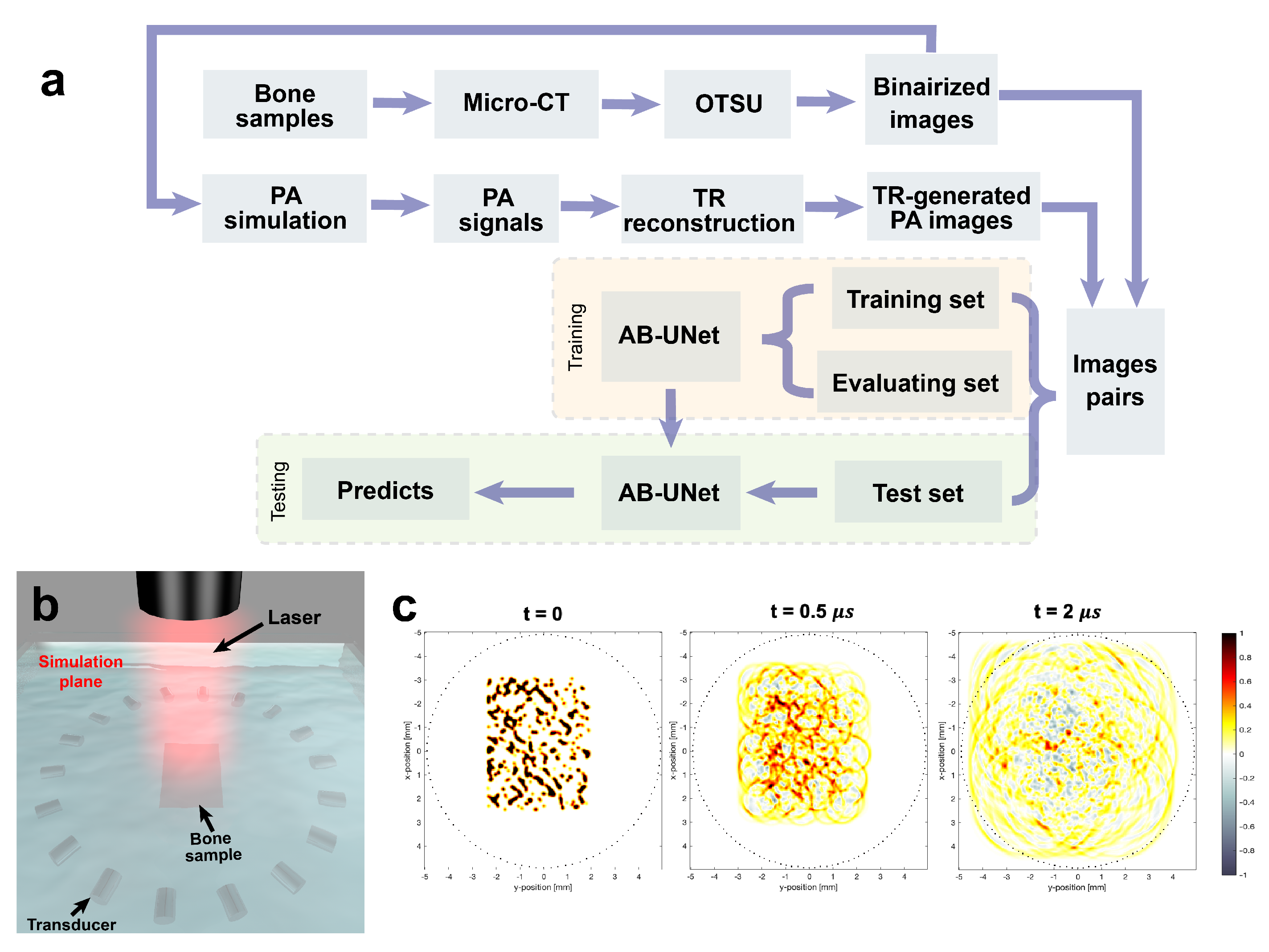
3.1. Dataset Generation

The bone samples used to prepare the dataset were collected from calcaneus of two human donators in Changhai Hospital, Shanghai. The age and sex of two human donators were unknown. The micro-structural image of the calcaneus bone specimen was obtained by micro-computed tomography (Skyscan 1076, Skyscan, Antwerp, Belgium), with a scanning resolution of 50 $\mathsf{\mu }$m. Then, a binary processing was implemented through an automatic threshold method OTSU to distinguish the trabecular bone from background [75]. The binarized micro-CT images of a cross-section in human calcaneus bone was used as the PA source. In the binarized micro-CT images, the white part is considered as the bone absorber with the initial PA pressure set as 1, while the black part was filled by water with the initial PA set as 0, simulating the initial pressure of trabecular bone produced by thermoelastic expansion when laser irradiates the bone sample. The propagating process of PA waves in bone was simulated by k-wave MATLAB toolbox, based on a space pseudo-spectral time domain solution to coupled first-order acoustic equations [69]. Then, detected PA signals were utilized to reconstruct images by TR, as shown in Figure 3.

For the PA imaging simulation setup, the computation domain was set as 10 × 10 mm${}^2$, where a circle of 128 ultrasound transducers with a radius of 4.9 mm is placed. An additional 2 mm perfectly matched layer was added to enclose the computational domain. We set the SOS and the density of the bone trabecula as 4000 m/s and 2000 kg/m${}^3$, respectively, while those of soft tissue (bone marrow) were 1500 m/s and 1000 kg/m${}^3$, respectively [39,76]. The center frequency of the transducer was taken as 7 MHz. The simulation time was set to 5 $\mathsf{\mu }$s, and the temporal sampling step was set to 3 ns.

Through TR, direct reconstruction images of bone were obtained, based on PA signals recorded. In TR settings, the average SOS and density of the medium used for PA image reconstruction were set to be the same as soft tissue 1500 m/s and 1000 kg/m${}^3$.

3.2. Training on Simulation Data

The CNN-based approach aims to extract features from low-quality images, then mapping those feature vectors to corresponding high dimensional space of high-resolution images. Therefore, by training the network through minimizing the loss function of initial direct reconstruction image $p_i^{*}$ and ground truth image $p_i$, problems like blurring, noisy patches, and modeling error from traditional PA reconstruction algorithms can be significantly mitigated. The optimization rule is expressed as follows [77]:

$$\underset{\mathsf{\Theta }}{argmin}L\left(f\left(p_i^{*};\mathsf{\Theta }\right)-p_i\right)$$

(9)

where L denotes the loss function of training data pairs $\left(p_i^{*},p_i\right)$. Parameter matrix $\mathsf{\Theta }$ is defined as the combination of weight matrix W and bias matrix B, represented by $\mathsf{\Theta }\triangleq W\circ B\triangleq \left(w_1\circ b_1\right)\circ \left(w_2\circ b_2\right)\circ \cdots \circ \left(w_l,b_l\right)$. Here, the substitute l denotes the layer of CNN.

For our network framework, significantly blurred and inaccurate modeling TR-reconstructed calcaneus images with gray transforming ${p_i}^{*}\in {\mathbb{R}}^{1\times 512\times 512}$ were fed in as the input, and binarized micro-CT images $p_i\in {\mathbb{R}}^{1\times 512\times 512}$ was taken as ground truth labels. Overall, 3800 collected micro-CT calcaneus scans were simulated to generate a set of pairs $\left(p_i^{*},p_i\right)$. Depending on the proportion of 60%, 20% and 20%, the dataset was divided into training set (2280 pairs), evaluating set (760 pairs) and test set (760 pairs). The resolution of all images is 512 × 512 pixels.

We implement our experiments on PyTorch [78], using an Intel Xeon Gold 6130 CPU and a Nvidia Quadro P4000 GPU. The training is run with Adam for 100 epochs, with a learning rate of 0.001 and batch size of 2.

4. Results

4.1. Reconstruction Results of Examples

Figure 4 presents visual results for calcaneus PA signal reconstruction by TR reconstruction and trained AB-U-Net.The cortical bone corresponds to the outer boundaries of the bone region, while the inner bone tissues are all cancellous bone. TR-reconstructed images show that the area of cortical bones is restored. However, there are significantly blurring and missing details at the inner part of the bone. It shows that, although TR tends to compensate for the perturbation caused by inhomogeneous medium to some extent, problems like strong scattering and the variation of sound speed are still unsolved and result in serious artifacts. In contrast, the AB-U-Net method successfully removes artifacts and restores the high-frequency information, such as the micro-structure of the trabecular bone. Compared with TR, the CNN-based network provides significant improvement in PSNR and SSIM, i.e., SSIM of sample 1 increases from 0.62 to 0.88, indicating an accurate modeling of the initial pressure.

The effect of the attention mechanism has been studied. Two types of CNN frameworks—U-Net and attention U-Net—were added to compare the reconstruction performance, shown in Figure 5. In addition, local details of a selected region were zoomed for a clearer interpretation. In the area with complex bone trabeculae, the initial pressure reconstructed by AB-U-Net (Figure 5d) is the best, as most of the micro-structures are well restored without inaccurate extra information.

To compare globally, SSIM-maps of results corresponding to three CNN models and TR are utilized, illustrating the SSIM value of each pixel on reconstructed PA images [79], as seen in Figure 6. It is noticeable that yellow areas (low SSIM) of AB-U-Net (Figure 6d) are the smallest, which represents better performance than the others. In addition, Figure 6b,c illustrate that the result of Attention U-Net is also better than that of U-Net, indicating that the added attention module helps to focus bone micro-structure information effectively. For PA imaging of bone tissue, it is suggested to add the attention module into the feature extraction part instead of in the decoder part.

4.2. Results of Global Test Set

To be more general, PSNR and SSIM for all test samples from the test set through different networks are listed in

Table 1. PSNR and SSIM under reconstructed images on Test Set.

Methods	Test Set (760 Samples)
	PSNR (dB)	SSIM
Time Reversal	12 ± 2.16	0.65 ± 0.09
U-Net	15.6 ± 1.97	0.81 ± 0.00
Attention U-Net	15.67 ± 1.95	0.81 ± 0.00
AB-U-Net	15.83 ± 2.04	0.82 ± 0.00

. CNN-based approaches achieve obviously better performance than TR, with PSNR and SSIM increased by more than 3 dB and 0.15, respectively. In comparison, among three CNN models, AB-U-Net performs the best satisfactory bone reconstruction. The evaluation indexes of U-Net are lower than others embedded with attention blocks. We believe that the attention mechanism is helpful to enhance model sensitivity and prediction accuracy.

There are perturbations of TR method between different bone samples, where the standard deviation of PSNR and SSIM go to 2.16 dB and 0.09 in the test set. Interestingly, after TR-obtained images processed by CNN, better robustness is achieved, i.e., a negligible variation of SSIM in Table 1. This result demonstrates that the post-processing method is more robust and shows its possibility to improve the image quality caused by the object structure and experimental conditions.

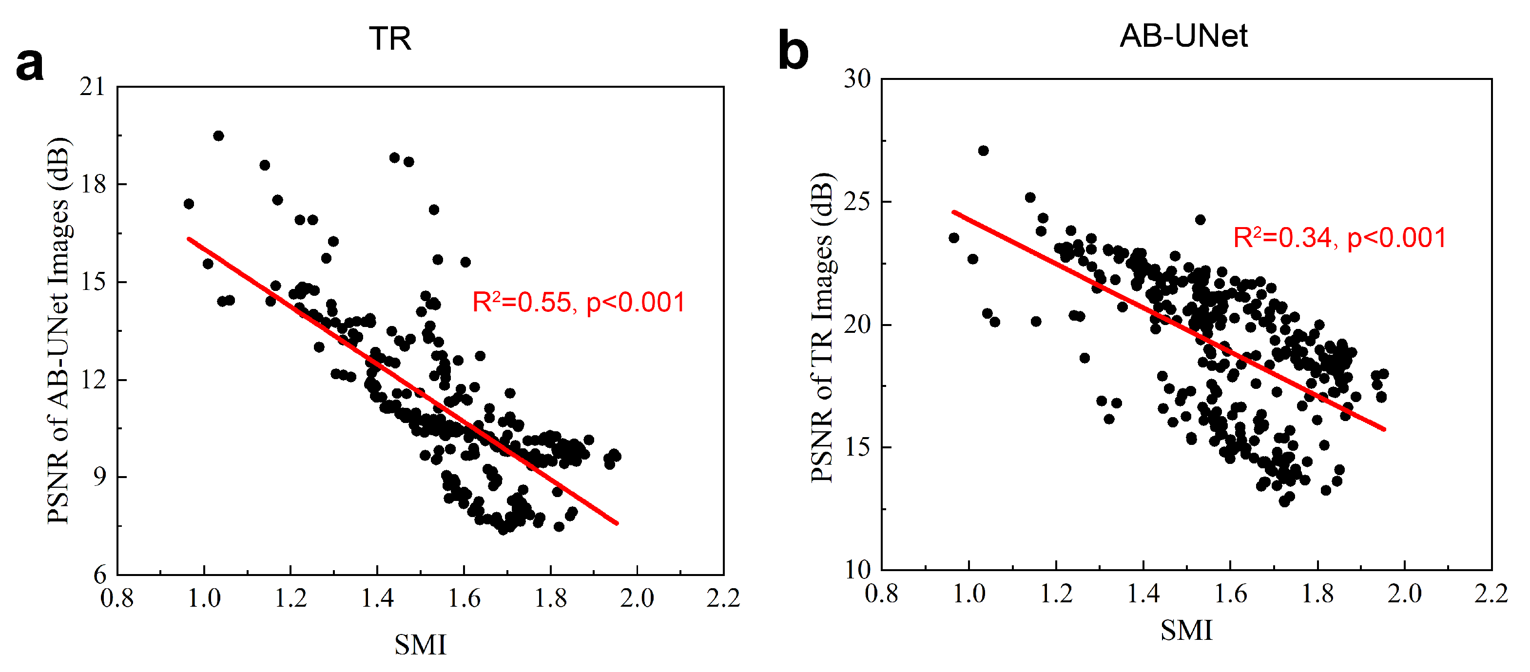
4.3. Statistical Significance Tests on the Results

Normal distribution tests were performed on the PSNR and SSIM values of all test images using a one-sample Kolmogorov–-Smirnov test (KS test) [80]. Comparing the empirical cumulative distribution function (CDF) of measured data with the predicted CDF of a normal model with normal-distribution-fitted parameters, the KS test rejected the null hypothesis at the 0.05 significance level, which indicated that the PSNR and SSIM values were not normally distributed. Since the PSNR and SSIM did not follow a normal distribution, a Wilcoxon signed-ranks test was used to test the significance of the improvement in PSNR and SSIM values for the proposed AB-U-Net reconstruction [81]. As shown in Figure 7, the AB-U-Net method showed a statistically improvement in reconstruction performance, with PSNR and SSIM significantly higher than those from TR, U-Net and Attention U-Net reconstructions (p < 0.05). In addition, the U-Net and attention U-Net also provided significant improvements in reconstruction performance than the TR method (p < 0.05). However, without a statistically significant improvement in the SSIM value (p > 0.05), the attention U-Net did not outperform the traditional U-Net for PA bone imaging.

5. Discussion

In this study, we investigated a method for PA bone imaging through deep learning post-processing. In traditional PA imaging, Fourier-domain and time-domain algorithms are proposed for initial pressure reconstruction [82,83,84,85]. Strict boundary conditions and the assumption of a constant SOS limit their applications in bone imaging [40]. In addition, most of the bone samples consist of cortical and trabecular bones. Considering the complex propagation of the PA signal in the cortical bone and trabecular bone, the PA signal of the cortical bone is difficult to be distinguished directly from the PA signal of trabecular bone. Therefore, in the PA imaging of bone, the complex propagation modes in cortical and trabecular bone will lead to PA images with low resolution if we use the traditional reconstruction method of PA imaging.

Inspired by the performance boost of CNNs in medical imaging (i.e., low-dose CT [86] and magnetic resonance imaging (MRI) acceleration [87]), we adopted the method through combining CNN and direct PA reconstruction algorithms. As the existing PA imaging technology is unable to provide high-resolution reconstructed images for bone, binarized micro-CT images are utilized as labels. The TR method was employed to produce low-quality PA images as the input of CNN, and was implemented as a comparison. Although model-based approaches have been reported to restore the initial pressure of PA source more accurately, they are at the cost of computational time [65]. Results prove that the proposed method successfully removes artifacts and partly corrects calculation errors, and outputs PA images closed to original micro-CT scans, with an inner micro-structure well restored. This improved result illustrates the promising future of PA bone imaging, where bone micro-structure can be presented without the suffering of radiation from micro-CT.

Besides the performance boost, it seems that the AB-U-Net effect of different bone samples changes. As seen in Figure 4, the reconstruction of sample 3 is much better than that of sample 2, as PSNR is 19.46 dB versus 14.10 dB and SSIM is 0.92 versus 0.79. Table 1 also reveals a fluctuation in reconstruction quality, either of TR or AB-U-Net. In order to explore what causes the fluctuations, main parameters of bone properties were calculated for bone samples from test set were using the CT analyzer software suite (CTAn, version1.14.4.1, Skyscan, Antwerp, Belgium). Result suggests that the structure model index (SMI) of bone samples has a direct influence on the reconstruction results. The SMI value is an important indicator for the trabecular micro-structure, describing the structure model of trabecular bones (0 for an ideal plate structure and 3 for an ideal cylindrical rod structure) [88]. Figure 8 showed the relationship between SMI and PSNR of PA reconstructed images by TR (Figure 8a) and AB-U-Net (Figure 8b). The PSNR of PA images by two methods yields significantly negative correlations with SMI (R${}^2$ = 0.55, p < 0.001 and R${}^2$ = 0.34, p < 0.001). The performance of reconstruction improved as the SMI of cancellous bone samples decreased. Bones with smaller SMI mean that its structure is a more regular plate-like, while bones with bigger SMI means relatively complicated rod-like trabecula. Trabecular micro-structure complexity increases the difficulty of reconstruction tasks. On the other hand, for AB-U-Net, its performance is related to the original TR reconstruction. The accuracy of feature recognition and the following restoration of CNN is also decreased in the more complex bone micro-structure. However, in comparison to Figure 8a,b, the correlation between AB-U-Net method and SMI decreases, indicating a mitigation of interference from trabecular micro-structure complexity. When reconstructing bone samples with various micro-structure complexities, the result in Figure 8 shows that the anti-interference ability of AB-U-Net is better than that of TR with steadier image quality.

We studied the influence of attention blocks in CNN reconstruction. Depending on their capabilities to focus on important information, attention modules have improved the performance of CNNs in the field of computational versions [89]. It is reasonable to believe that the addition of this module will enhance the quality of reconstruction. In this study, we embedded CBAM into the typical U-Net and designed a new network: AB-U-Net. Besides, U-Net (without attention module) and attention U-Net (attention module in the decoder part) were added for comparison to investigate the effect. Results demonstrate that attention blocks embedded into feature extraction modules implicitly learn useful features and suppress feature activations in irrelevant regions. Thus, for the reconstruction task of bones with complex interior structures, it is better to employ attention blocks in the encoder part to enhance CNN’s ability feature representative.

One advantage of the trained CNNs for medical image reconstruction is their ability to restore relatively accurate information in a short time, which meets the need of fast imaging. Specifically, the comparisons of the computational complexities and reconstruction times of the three CNN networks are summarized in

Table 2. The computational complexities of cnn models.

Models	Params (M)	FLOPs (G)	Training Time (100 Epochs)	Testing Time (Single Image)
U-Net	31	184	23 h	3 s
Attention U-Net	34	266	1 d 8 h	3 s
AB-U-Net	95	329	2 d 20 h	5 s

. ‘Params’ represents the number of model parameters. ‘FLOPs’ are floating point numbers, understood as the amount of computation. The computations were performed using an Intel Xeon Gold 6130 CPU and a Nvidia Quadro P4000 GPU. The training times for CNNs were calculated using the training set of 2280 image pairs (512 × 512 resolution) for 100 epochs with the batch size of 2, and the testing times for the trained CNNs of a single PA image (reconstruction time) were given. As shown in Table 2, the computational complexity of AB-U-Net (329 GFLOPs) is higher than U-Net (184 GFLOPs) and attention U-Net (266 GFLOPs). The complex computation leads to the AB-U-Net need to reduce the batch size of training and undertake longer training time than the others. However, once the network training is completed, the reconstruction for single PA image of AB-U-Net only takes 5 s. Although the testing time of AB-U-Net is still longer than U-Net and Attention U-Net, it is acceptable at the cost of only 2 s additional to achieve better performance.

A limitation of this study is that simulation data were used for training and testing the CNN framework for PA bone reconstruction. As a data-driven method, the CNN model requires a large amount of data for training and learning implicit information. It is not very effective and extremely time-consuming to measure massive in vitro or in vivo PA experimental signals from varied bone conditions. However, simulations were quite helpful and effective to generate sufficient PA data for training the CNN models. The simulation results showed that the proposed AB-U-Net significantly improved the quality of PA reconstructed bone images. To better combine the simulations with practical experiments, we will perform in vitro and in vivo experiments to validate the effect of CNN reconstruction in PA bone images. Transfer learning could be used to adopt and apply the simulation-trained CNN models to in vitro and in vivo experimental conditions [90]. With the best use of previously marked data, transfer learning can effectively shorten training time and improving model accuracy [90]. Another limitation is that as our study is an initial study, no in vivo environmental condition of PA simulation is considered. The numerical model we employed makes simplifications compared to real bone tissue, i.e., without considering several tissue layers on top of the bone (e.g., skin, fat) and vasculatures within the bone. When laser irradiates the tissue, the measured bone generated PA signals may be affected by ultrasonic attenuation and scattering effects in soft tissue overlying the bone. In this case, the reconstruction performance of both TR method and AB-U-Net might be decreased. However, through training the dataset including PA images of bone with several tissue layers, AB-U-Net is likely to extract and mitigate artifacts of soft tissues, and achieves a satisfying reconstruction quality. The analysis of bones with several tissue layers will be investigated in the follow-up work. We believe that deep learning technology can help photoacoustic technology in the accurate imaging of bone micro-structure, and then promote the development of bone disease detection.

6. Conclusions

In this paper, we proposed a new CNN framework named AB-U-Net for reconstructing bone micro-structure of numerically simulated PA data estimated from micro-CT data. Results demonstrate that the post-processing method can significantly improve the quality of PA reconstructed images, by removing artifacts and compensating computational errors. Additionally, relationships between reconstruction quality and SMI of cancellous bone samples are also investigated. In future work, a series of PA in vitro experiments are expected to be implemented to further validate our simulation results.

References

1. Griffith, J.F.; Yeung, D.K.; Antonio, G.E.; Lee, F.K.; Hong, A.W.; Wong, S.Y.; Lau, E.M.; Leung, P.C. Vertebral bone mineral density, marrow perfusion, and fat content in healthy men and men with osteoporosis: Dynamic contrast-enhanced MR imaging and MR spectroscopy. Radiology 2005, 236, 945–951. [Google Scholar] [CrossRef]
2. Harvey, N.; Dennison, E.; Cooper, C. Osteoporosis: Impact on health and economics. Nat. Rev. Rheumatol. 2010, 6, 99. [Google Scholar] [CrossRef]
3. Sim, L.; Van Doorn, T. Radiographic measurement of bone mineral: Reviewing dual energy X-ray absorptiometry. Australas. Phys. Eng. Sci. Med. 1995, 18, 65. [Google Scholar]
4. Blake, G.M.; Fogelman, I. Technical principles of dual energy x-ray absorptiometry. In Seminars in Nuclear Medicine; Elsevier: Amsterdam, The Netherlands, 1997; Volume 27, pp. 210–228. [Google Scholar]
5. Pisani, P.; Renna, M.D.; Conversano, F.; Casciaro, E.; Muratore, M.; Quarta, E.; Di Paola, M.; Casciaro, S. Screening and early diagnosis of osteoporosis through X-ray and ultrasound based techniques. World J. Radiol. 2013, 5, 398. [Google Scholar] [CrossRef] [PubMed]
6. Laugier, P.; Haïat, G. Bone Quantitative Ultrasound; Springer: Berlin/Heidelberg, Germany, 2011; Volume 576. [Google Scholar]
7. Fratzl, P.; Gupta, H.; Paschalis, E.; Roschger, P. Structure and mechanical quality of the collagen–mineral nano-composite in bone. J. Mater. Chem. 2004, 14, 2115–2123. [Google Scholar] [CrossRef]
8. Genant, H.; Engelke, K.; Prevrhal, S. Advanced CT bone imaging in osteoporosis. Rheumatology 2008, 47, iv9–iv16. [Google Scholar] [CrossRef] [PubMed] [Green Version]
9. Njeh, C.; Boivin, C.; Langton, C. The role of ultrasound in the assessment of osteoporosis: A review. Osteoporos. Int. 1997, 7, 7–22. [Google Scholar] [CrossRef] [PubMed]
10. Kaufman, J.J.; Einhorn, T.A. Ultrasound assessment of bone. J. Bone Miner. Res. 1993, 8, 517–525. [Google Scholar] [CrossRef] [PubMed]
11. Liu, C.; Dong, R.; Li, B.; Li, Y.; Xu, F.; Ta, D.; Wang, W. Ultrasonic backscatter characterization of cancellous bone using a general Nakagami statistical model. Chin. Phys. B 2019, 28, 024302. [Google Scholar] [CrossRef]
12. Liu, C.; Li, B.; Li, Y.; Mao, W.; Chen, C.; Zhang, R.; Ta, D. Ultrasonic Backscatter Difference Measurement of Bone Health in Preterm and Term Newborns. Ultrasound Med. Biol. 2020, 46, 305–314. [Google Scholar] [CrossRef]
13. Li, Y.; Li, B.; Li, Y.; Liu, C.; Xu, F.; Zhang, R.; Ta, D.; Wang, W. The ability of ultrasonic backscatter parametric imaging to characterize bovine trabecular bone. Ultrason. Imaging 2019, 41, 271–289. [Google Scholar] [CrossRef] [PubMed]
14. Liu, C.; Ta, D.; Fujita, F.; Hachiken, T.; Matsukawa, M.; Mizuno, K.; Wang, W. The relationship between ultrasonic backscatter and trabecular anisotropic microstructure in cancellous bone. J. Appl. Phys. 2014, 115, 064906. [Google Scholar] [CrossRef]
15. Wear, K.A. Mechanisms of Interaction of Ultrasound With Cancellous Bone: A Review. IEEE Trans. Ultrason. Ferroelectr. Freq. Control. 2019, 67, 454–482. [Google Scholar] [CrossRef]
16. Chaffaı, S.; Peyrin, F.; Nuzzo, S.; Porcher, R.; Berger, G.; Laugier, P. Ultrasonic characterization of human cancellous bone using transmission and backscatter measurements: Relationships to density and microstructure. Bone 2002, 30, 229–237. [Google Scholar] [CrossRef]
17. Liu, C.; Li, B.; Diwu, Q.; Li, Y.; Zhang, R.; Ta, D.; Wang, W. Relationships of ultrasonic backscatter with bone densities and microstructure in bovine cancellous bone. IEEE Trans. Ultrason. Ferroelectr. Freq. Control. 2018, 65, 2311–2321. [Google Scholar] [CrossRef]
18. Guillaume, R.; Pieter, K.; Didier, C.; Pascal, L. In vivo ultrasound imaging of the bone cortex. Phys. Med. Biol. 2018, 63, 125010. [Google Scholar]
19. Xu, M.; Wang, L.V. Photoacoustic imaging in biomedicine. Rev. Sci. Instruments 2006, 77, 041101. [Google Scholar] [CrossRef] [Green Version]
20. Beard, P. Biomedical photoacoustic imaging. Interface Focus 2011, 1, 602–631. [Google Scholar] [CrossRef]
21. Cao, F.; Qiu, Z.; Li, H.; Lai, P. Photoacoustic imaging in oxygen detection. Appl. Sci. 2017, 7, 1262. [Google Scholar] [CrossRef] [Green Version]
22. Feng, T.; Zhu, Y.; Morris, R.; Kozloff, K.; Wang, X. Functional Photoacoustic and Ultrasonic Assessment of Osteoporosis: A Clinical Feasibility Study. Biomed. Eng. Front. 2020, 2020, 15. [Google Scholar]
23. Wang, L.V.; Hu, S. Photoacoustic tomography: In vivo imaging from organelles to organs. Science 2012, 335, 1458–1462. [Google Scholar] [CrossRef] [PubMed] [Green Version]
24. Hoelen, C.; De Mul, F.; Pongers, R.; Dekker, A. Three-dimensional photoacoustic imaging of blood vessels in tissue. Opt. Lett. 1998, 23, 648–650. [Google Scholar] [CrossRef] [PubMed]
25. Jansen, K.; Van Der Steen, A.F.; van Beusekom, H.M.; Oosterhuis, J.W.; van Soest, G. Intravascular photoacoustic imaging of human coronary atherosclerosis. Opt. Lett. 2011, 36, 597–599. [Google Scholar] [CrossRef] [PubMed] [Green Version]
26. Kruger, R.A.; Lam, R.B.; Reinecke, D.R.; Del Rio, S.P.; Doyle, R.P. Photoacoustic angiography of the breast. Med. Phys. 2010, 37, 6096–6100. [Google Scholar] [CrossRef]
27. Mallidi, S.; Luke, G.P.; Emelianov, S. Photoacoustic imaging in cancer detection, diagnosis, and treatment guidance. Trends Biotechnol. 2011, 29, 213–221. [Google Scholar] [CrossRef] [Green Version]
28. Rao, A.P.; Bokde, N.; Sinha, S. Photoacoustic imaging for management of breast cancer: A literature review and future perspectives. Appl. Sci. 2020, 10, 767. [Google Scholar] [CrossRef] [Green Version]
29. Lashkari, B.; Mandelis, A. Coregistered photoacoustic and ultrasonic signatures of early bone density variations. J. Biomed. Opt. 2014, 19, 036015. [Google Scholar] [CrossRef]
30. Feng, T.; Kozloff, K.M.; Tian, C.; Perosky, J.E.; Hsiao, Y.S.; Du, S.; Yuan, J.; Deng, C.X.; Wang, X. Bone assessment via thermal photo-acoustic measurements. Opt. Lett. 2015, 40, 1721–1724. [Google Scholar] [CrossRef] [Green Version]
31. Gu, C.; Katti, D.R.; Katti, K.S. Microstructural and photoacoustic infrared spectroscopic studies of human cortical bone with osteogenesis imperfecta. JOM 2016, 68, 1116–1127. [Google Scholar] [CrossRef]
32. Wang, X.; Feng, T.; Cao, M.; Perosky, J.E.; Kozloff, K.; Cheng, Q.; Yuan, J. Photoacoustic measurement of bone health: A study for clinical feasibility. In Proceedings of the 2016 IEEE International Ultrasonics Symposium (IUS), Tours, France, 18–21 September 2016; pp. 1–4. [Google Scholar]
33. Wang, X.; Chamberland, D.L.; Jamadar, D.A. Noninvasive photoacoustic tomography of human peripheral joints toward diagnosis of inflammatory arthritis. Opt. Lett. 2007, 32, 3002–3004. [Google Scholar] [CrossRef]
34. Yang, L.; Lashkari, B.; Tan, J.W.; Mandelis, A. Photoacoustic and ultrasound imaging of cancellous bone tissue. J. Biomed. Opt. 2015, 20, 076016. [Google Scholar] [CrossRef] [PubMed]
35. Merrill, J.A.; Wang, S.; Zhao, Y.; Arellano, J.; Xiang, L. Photoacoustic microscopy for bone microstructure analysis. In Proceedings of the Biophotonics and Immune Responses XV. International Society for Optics and Photonics, Bellingham, WA, USA, 1–6 February 2020; Volume 11241, p. 112410H. [Google Scholar]
36. Syahrom, A.; bin Mohd Szali, M.A.F.; Harun, M.N.; Öchsner, A. Cancellous bone. In Cancellous Bone; Springer: Berlin/Heidelberg, Germany, 2018; pp. 7–20. [Google Scholar]
37. Shim, V.; Yang, L.; Liu, J.; Lee, V. Characterisation of the dynamic compressive mechanical properties of cancellous bone from the human cervical spine. Int. J. Impact Eng. 2005, 32, 525–540. [Google Scholar] [CrossRef]
38. Hans, D.; Wu, C.; Njeh, C.; Zhao, S.; Augat, P.; Newitt, D.; Link, T.; Lu, Y.; Majumdar, S.; Genant, H. Ultrasound velocity of trabecular cubes reflects mainly bone density and elasticity. Calcif. Tissue Int. 1999, 64, 18–23. [Google Scholar] [CrossRef] [PubMed]
39. Haiat, G.; Lhemery, A.; Renaud, F.; Padilla, F.; Laugier, P.; Naili, S. Velocity dispersion in trabecular bone: Influence of multiple scattering and of absorption. J. Acoust. Soc. Am. 2008, 124, 4047–4058. [Google Scholar] [CrossRef] [PubMed]
40. Xu, Y.; Wang, L.V. Effects of acoustic heterogeneity in breast thermoacoustic tomography. IEEE Trans. Ultrason. Ferroelectr. Freq. Control. 2003, 50, 1134–1146. [Google Scholar] [PubMed] [Green Version]
41. Haltmeier, M. Sampling conditions for the circular radon transform. IEEE Trans. Image Process. 2016, 25, 2910–2919. [Google Scholar] [CrossRef] [PubMed]
42. Wang, J.; Zhao, Z.; Song, J.; Chen, G.; Nie, Z.; Liu, Q.H. Reducing the effects of acoustic heterogeneity with an iterative reconstruction method from experimental data in microwave induced thermoacoustic tomography. Med. Phys. 2015, 42, 2103–2112. [Google Scholar] [CrossRef] [PubMed]
43. Jin, X.; Wang, L.V. Thermoacoustic tomography with correction for acoustic speed variations. Phys. Med. Biol. 2006, 51, 6437. [Google Scholar] [CrossRef]
44. Zhang, J.; Anastasio, M.A. Reconstruction of speed-of-sound and electromagnetic absorption distributions in photoacoustic tomography. In Photons Plus Ultrasound: Imaging and Sensing 2006: The Seventh Conference on Biomedical Thermoacoustics, Optoacoustics, and Acousto-optics; International Society for Optics and Photonics: Bellingham, WA, USA, 2006; Volume 6086, p. 608619. [Google Scholar]
45. Rui, W.; Liu, Z.; Tao, C.; Liu, X. Reconstruction of Photoacoustic Tomography Inside a Scattering Layer Using a Matrix Filtering Method. Appl. Sci. 2019, 9, 2071. [Google Scholar] [CrossRef] [Green Version]
46. LeCun, Y.; Bengio, Y.; Hinton, G. Deep learning. Nature 2015, 521, 436–444. [Google Scholar] [CrossRef]
47. Li, Q.; Cai, W.; Wang, X.; Zhou, Y.; Feng, D.D.; Chen, M. Medical image classification with convolutional neural network. In Proceedings of the 2014 13th International Conference on Control Automation Robotics & Vision (ICARCV), Singapore, 10–12 December 2014; pp. 844–848. [Google Scholar]
48. Chan, T.H.; Jia, K.; Gao, S.; Lu, J.; Zeng, Z.; Ma, Y. PCANet: A simple deep learning baseline for image classification? IEEE Trans. Image Process. 2015, 24, 5017–5032. [Google Scholar] [CrossRef] [PubMed] [Green Version]
49. Krizhevsky, A.; Sutskever, I.; Hinton, G.E. Imagenet classification with deep convolutional neural networks. In Proceedings of the Advances in Neural Information Processing Systems, Lake Tahoe, NV, USA, 3–6 December 2012; pp. 1097–1105. [Google Scholar]
50. Yu, S.; Jia, S.; Xu, C. Convolutional neural networks for hyperspectral image classification. Neurocomputing 2017, 219, 88–98. [Google Scholar] [CrossRef]
51. Dong, C.; Loy, C.C.; He, K.; Tang, X. Image super-resolution using deep convolutional networks. IEEE Trans. Pattern Anal. Mach. Intell. 2015, 38, 295–307. [Google Scholar] [CrossRef] [PubMed] [Green Version]
52. Kim, J.; Kwon Lee, J.; Mu Lee, K. Accurate image super-resolution using very deep convolutional networks. In Proceedings of the IEEE Conference on Computer Vision and Pattern Recognition, Las Vegas, NV, USA, 26 June–1 July 2016; pp. 1646–1654. [Google Scholar]
53. Zhang, Y.; Tian, Y.; Kong, Y.; Zhong, B.; Fu, Y. Residual dense network for image super-resolution. In Proceedings of the IEEE Conference on Computer Vision and Pattern Recognition, Salt Lake City, UT, USA, 18–23 June 2018; pp. 2472–2481. [Google Scholar]
54. Higaki, T.; Nakamura, Y.; Tatsugami, F.; Nakaura, T.; Awai, K. Improvement of image quality at CT and MRI using deep learning. Jpn. J. Radiol. 2019, 37, 73–80. [Google Scholar] [CrossRef]
55. Urase, Y.; Nishio, M.; Ueno, Y.; Kono, A.K.; Sofue, K.; Kanda, T.; Maeda, T.; Nogami, M.; Hori, M.; Murakami, T. Simulation Study of Low-Dose Sparse-Sampling CT with Deep Learning-Based Reconstruction: Usefulness for Evaluation of Ovarian Cancer Metastasis. Appl. Sci. 2020, 10, 4446. [Google Scholar] [CrossRef]
56. Liang, D.; Cheng, J.; Ke, Z.; Ying, L. Deep magnetic resonance image reconstruction: Inverse problems meet neural networks. IEEE Signal Process. Mag. 2020, 37, 141–151. [Google Scholar] [CrossRef]
57. Kovács, P.; Lehner, B.; Thummerer, G.; Mayr, G.; Burgholzer, P.; Huemer, M. Deep learning approaches for thermographic imaging. J. Appl. Phys. 2020, 128, 155103. [Google Scholar] [CrossRef]
58. Ramzi, Z.; Ciuciu, P.; Starck, J.L. Benchmarking MRI Reconstruction Neural Networks on Large Public Datasets. Appl. Sci. 2020, 10, 1816. [Google Scholar] [CrossRef] [Green Version]
59. Yang, C.; Lan, H.; Gao, F.; Gao, F. Deep learning for photoacoustic imaging: A survey. arXiv 2020, arXiv:2008.04221. [Google Scholar]
60. Hauptmann, A.; Cox, B. Deep Learning in Photoacoustic Tomography: Current approaches and future directions. J. Biomed. Opt. 2020, 25, 112903. [Google Scholar] [CrossRef]
61. Manwar, R.; Li, X.; Mahmoodkalayeh, S.; Asano, E.; Zhu, D.; Avanaki, K. Deep learning protocol for improved photoacoustic brain imaging. J. Biophotonics 2020, 13, e202000212. [Google Scholar] [CrossRef]
62. Allman, D.; Reiter, A.; Bell, M.A.L. Photoacoustic source detection and reflection artifact removal enabled by deep learning. IEEE Trans. Med. Imaging 2018, 37, 1464–1477. [Google Scholar] [CrossRef] [PubMed]
63. Davoudi, N.; Deán-Ben, X.L.; Razansky, D. Deep learning optoacoustic tomography with sparse data. Nat. Mach. Intell. 2019, 1, 453–460. [Google Scholar] [CrossRef]
64. Hariri, A.; Alipour, K.; Mantri, Y.; Schulze, J.P.; Jokerst, J.V. Deep learning improves contrast in low-fluence photoacoustic imaging. Biomed. Opt. Express 2020, 11, 3360–3373. [Google Scholar] [CrossRef]
65. Hauptmann, A.; Lucka, F.; Betcke, M.; Huynh, N.; Adler, J.; Cox, B.; Beard, P.; Ourselin, S.; Arridge, S. Model-based learning for accelerated, limited-view 3-d photoacoustic tomography. IEEE Trans. Med. Imaging 2018, 37, 1382–1393. [Google Scholar] [CrossRef] [Green Version]
66. Jin, K.H.; McCann, M.T.; Froustey, E.; Unser, M. Deep convolutional neural network for inverse problems in imaging. IEEE Trans. Image Process. 2017, 26, 4509–4522. [Google Scholar] [CrossRef] [Green Version]
67. Chen, L.; Zhang, H.; Xiao, J.; Nie, L.; Shao, J.; Liu, W.; Chua, T.S. Sca-cnn: Spatial and channel-wise attention in convolutional networks for image captioning. In Proceedings of the IEEE Conference on Computer Vision and Pattern Recognition, Honolulu, HI, USA, 21–26 July 2017; pp. 5659–5667. [Google Scholar]
68. Ronneberger, O.; Fischer, P.; Brox, T. U-net: Convolutional networks for biomedical image segmentation. In Proceedings of the International Conference on Medical Image Computing and Computer-Assisted Intervention, Munich, Germany, 5–9 October 2015; pp. 234–241. [Google Scholar]
69. Treeby, B.E.; Cox, B.T. k-Wave: MATLAB toolbox for the simulation and reconstruction of photoacoustic wave fields. J. Biomed. Opt. 2010, 15, 021314. [Google Scholar] [CrossRef]
70. Woo, S.; Park, J.; Lee, J.Y.; So Kweon, I. Cbam: Convolutional block attention module. In Proceedings of the European Conference on Computer Vision (ECCV), Munich, Germany, 8–14 September 2018; pp. 3–19. [Google Scholar]
71. Milletari, F.; Navab, N.; Ahmadi, S.A. V-net: Fully convolutional neural networks for volumetric medical image segmentation. In Proceedings of the 2016 fourth international conference on 3D vision (3DV), Stanford, CA, USA, 25–28 October 2016; pp. 565–571. [Google Scholar]
72. Andrew, G.; Gao, J. Scalable training of L 1-regularized log-linear models. In Proceedings of the 24th International Conference on Machine Learning, Corvallis, OR, USA, 20–24 June 2007; pp. 33–40. [Google Scholar]
73. Hore, A.; Ziou, D. Image quality metrics: PSNR vs. SSIM. In Proceedings of the 2010 20th International Conference on Pattern Recognition, Istanbul, Turkey, 23–26 August 2010; pp. 2366–2369. [Google Scholar]
74. Oktay, O.; Schlemper, J.; Folgoc, L.L.; Lee, M.; Heinrich, M.; Misawa, K.; Mori, K.; McDonagh, S.; Hammerla, N.Y.; Kainz, B. Attention u-net: Learning where to look for the pancreas. arXiv 2018, arXiv:1804.03999. [Google Scholar]
75. Otsu, N. A threshold selection method from gray-level histograms. IEEE Trans. Syst. Man, Cybern. 1979, 9, 62–66. [Google Scholar] [CrossRef] [Green Version]
76. Aula, A.; Töyräs, J.; Hakulinen, M.; Jurvelin, J. Effect of bone marrow on acoustic properties of trabecular bone-3d finite difference modeling study. Ultrasound Med. Biol. 2009, 35, 308–318. [Google Scholar] [CrossRef]
77. Antholzer, S.; Haltmeier, M.; Nuster, R.; Schwab, J. Photoacoustic image reconstruction via deep learning. In Proceedings of the Photons Plus Ultrasound: Imaging and Sensing 2018. International Society for Optics and Photonics, San Diego, CA, USA, 19–23 August 2018; Volume 10494, p. 104944U. [Google Scholar]
78. Paszke, A.; Gross, S.; Massa, F.; Lerer, A.; Bradbury, J.; Chanan, G.; Killeen, T.; Lin, Z.; Gimelshein, N.; Antiga, L. Pytorch: An imperative style, high-performance deep learning library. In Proceedings of the Advances in Neural Information Processing Systems, Vancouver, BC, Canada, 8–14 December 2019; pp. 8026–8037. [Google Scholar]
79. Rehman, A.; Rostami, M.; Wang, Z.; Brunet, D.; Vrscay, E.R. SSIM-inspired image restoration using sparse representation. EURASIP J. Adv. Signal Process. 2012, 2012, 16. [Google Scholar] [CrossRef]
80. Mishra, P.; Pandey, C.M.; Singh, U.; Gupta, A.; Sahu, C.; Keshri, A. Descriptive statistics and normality tests for statistical data. Ann. Card. Anaesth. 2019, 22, 67. [Google Scholar] [PubMed]
81. Trawiński, B.; Smętek, M.; Telec, Z.; Lasota, T. Nonparametric statistical analysis for multiple comparison of machine learning regression algorithms. Int. J. Appl. Math. Comput. Sci. 2012, 22, 867–881. [Google Scholar] [CrossRef]
82. Xu, Y.; Feng, D.; Wang, L.V. Exact frequency-domain reconstruction for thermoacoustic tomography. I. Planar geometry. IEEE Trans. Med. Imaging 2002, 21, 823–828. [Google Scholar]
83. Xu, M.; Wang, L.V. Time-domain reconstruction for thermoacoustic tomography in a spherical geometry. IEEE Trans. Med. Imaging 2002, 21, 814–822. [Google Scholar]
84. Xu, Y.; Wang, L.V. Time reversal and its application to tomography with diffracting sources. Phys. Rev. Lett. 2004, 92, 033902. [Google Scholar] [CrossRef] [Green Version]
85. Xu, M.; Wang, L.V. Universal back-projection algorithm for photoacoustic computed tomography. Phys. Rev. E 2005, 71, 016706. [Google Scholar] [CrossRef] [Green Version]
86. Chen, H.; Zhang, Y.; Zhang, W.; Liao, P.; Li, K.; Zhou, J.; Wang, G. Low-dose CT via convolutional neural network. Biomed. Opt. Express 2017, 8, 679–694. [Google Scholar] [CrossRef]
87. Lee, D.; Yoo, J.; Tak, S.; Ye, J.C. Deep residual learning for accelerated MRI using magnitude and phase networks. IEEE Trans. Biomed. Eng. 2018, 65, 1985–1995. [Google Scholar] [CrossRef] [Green Version]
88. Arlot, M.E.; Burt-Pichat, B.; Roux, J.P.; Vashishth, D.; Bouxsein, M.L.; Delmas, P.D. Microarchitecture influences microdamage accumulation in human vertebral trabecular bone. J. Bone Miner. Res. 2008, 23, 1613–1618. [Google Scholar] [CrossRef]
89. Zhao, T.; Wu, X. Pyramid feature attention network for saliency detection. In Proceedings of the IEEE Conference on Computer Vision and Pattern Recognition, Long Beach, CA, USA, 16–20 June 2019; pp. 3085–3094. [Google Scholar]
90. Cheng, P.M.; Malhi, H.S. Transfer learning with convolutional neural networks for classification of abdominal ultrasound images. J. Digit. Imaging 2017, 30, 234–243. [Google Scholar] [CrossRef] [PubMed]
Figure 1. Illustration of proposed attention block U-net (AB-U-Net). time reversal (TR)-reconstructed images are fed into the encoder module where the attention blocks embedded. The reconstruction images are outputted through the decoder part.
Applsci 10 08089 g001
Figure 2. Schematic of the attention block. It contains two sequentially sub-modules: channel attention module and spatial attention module.
Applsci 10 08089 g002
Figure 3. (a) The schematic of the data generation process. (b) The diagram of the simulation of PA signal propagation. (c) k-wave setup and propagation process of photoacoustic (PA) waves from t = 0 to t = 2 μ s.
Applsci 10 08089 g003
Figure 4. (ai) Visual comparison of the performance in three examples based on TR and AB-U-Net. Each row represents a different bone sample, from top to bottom: sample 1, sample 2 and sample 3. Every column represents different method, from left to right: ground truth, time-reversal reconstructed and AB-U-Net.
Applsci 10 08089 g004
Figure 5. The example of performance comparison based on different convolution neural network (CNN) architectures: (a) Ground Truth, (b) U-Net, (c) Attention U-Net and (d) AB-U-Net. A red rectangle area is selected and zoomed to intuitively compare reconstruction effects for the complex bone trabeculae.
Applsci 10 08089 g005
Figure 6. Comparison of structural similarity (SSIM) map based on different CNN architectures: (a) Time Reversal, (b) U-Net, (c) Attention U-Net and (d) AB-U-Net. Yellow corresponds to reconstructed areas with low SSIM, which indicates the poor reconstruction performance.
Applsci 10 08089 g006
Figure 7. Wilcoxon test on (a) PSNR and (b) SSIM of four methods for test set. The mean value of each data is represented by the height of the bar. The error bar indicates the range of data.
Applsci 10 08089 g007
Figure 8. (a) Scatter plots of the relationship between SMI and the performance of TR reconstruction, and (b) performance of AB-U-Net reconstruction. The red lines are the fitting curves of linear regression, where R 2 is the coefficient of determination, and p is the possibility value.
Applsci 10 08089 g008