Detection and Identification of Malicious Cyber-Attacks in Connected and Automated Vehicles’ Real-Time Sensors

 ,
,  , ,
, ,  , and
, and 
Abstract
1. Introduction
- Instant I: This form of anomaly is simulated as a Gaussian random variable.
- Bias B: The anomaly is simulated by adding a temporarily offset to the observation, which is different when compared with the normal sensor reading.
- Gradual Drift G: This type of anomaly is simulated by linearly adding set of values in decreasing/increasing order to the base sensor values.
Contributions
- We develop anomaly detection approach through combining Bayesian deep learning (BDL), with a well established filter techniques, discrete wavelet transform (DWT), applied to time series BSMs data obtained from multiple sensors.
- Extensive experimental evaluations are carried out to investigate the effects of anomaly type, magnitude, duration in single and multiple anomaly scenario (unseen anomaly) in real world BSMs dataset.
- We investigate the sensitivity and distribution of the selected anomalous BSMs sensor values used in the experiment with or without DWT.
2. Related Work
3. Misbehavior Scenarios and Alert Types
3.1. Emergency Electronic Brake Light (EEBL)
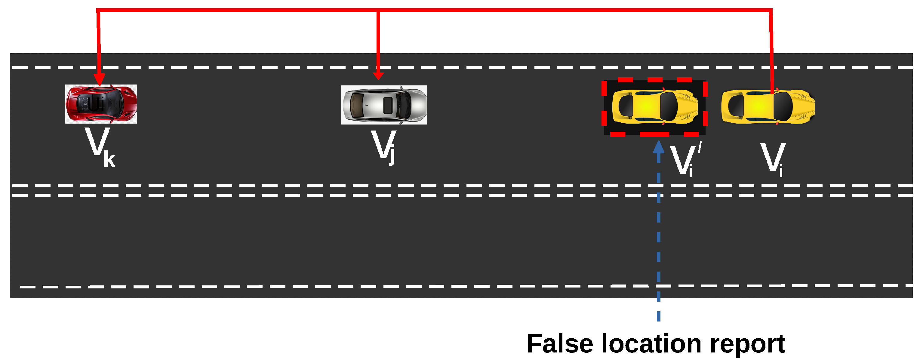
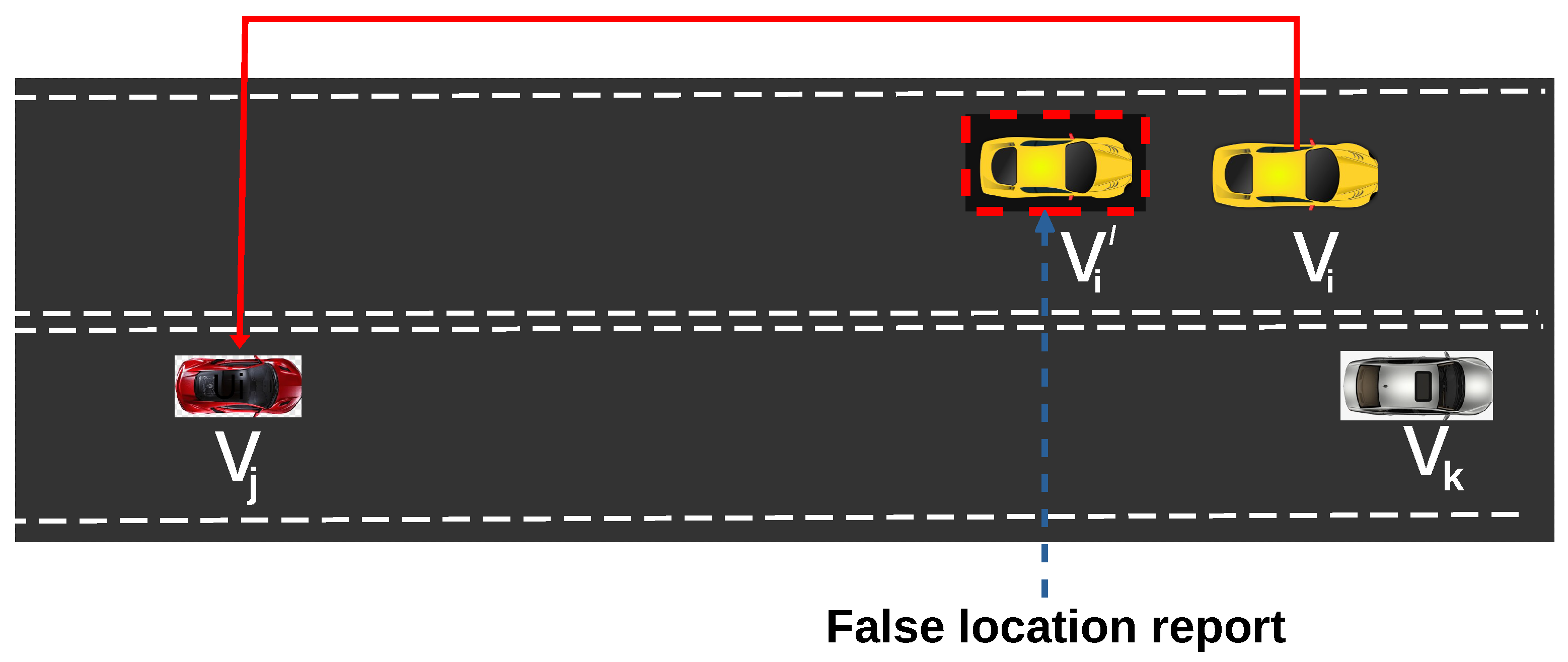
3.2. Change of Lane (CoL)
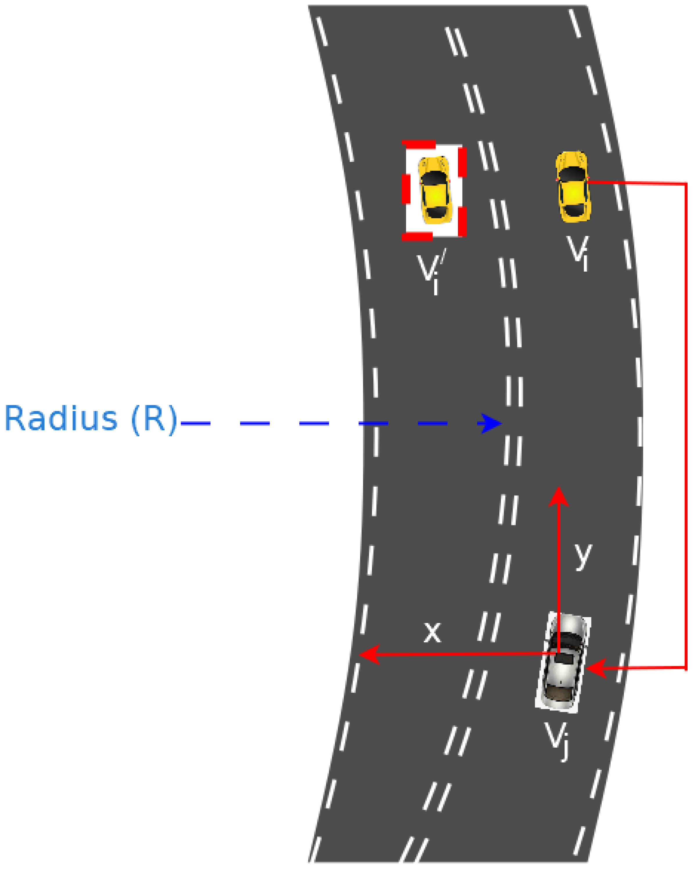
3.3. Path Deviation Alert (PDA)
4. Methods
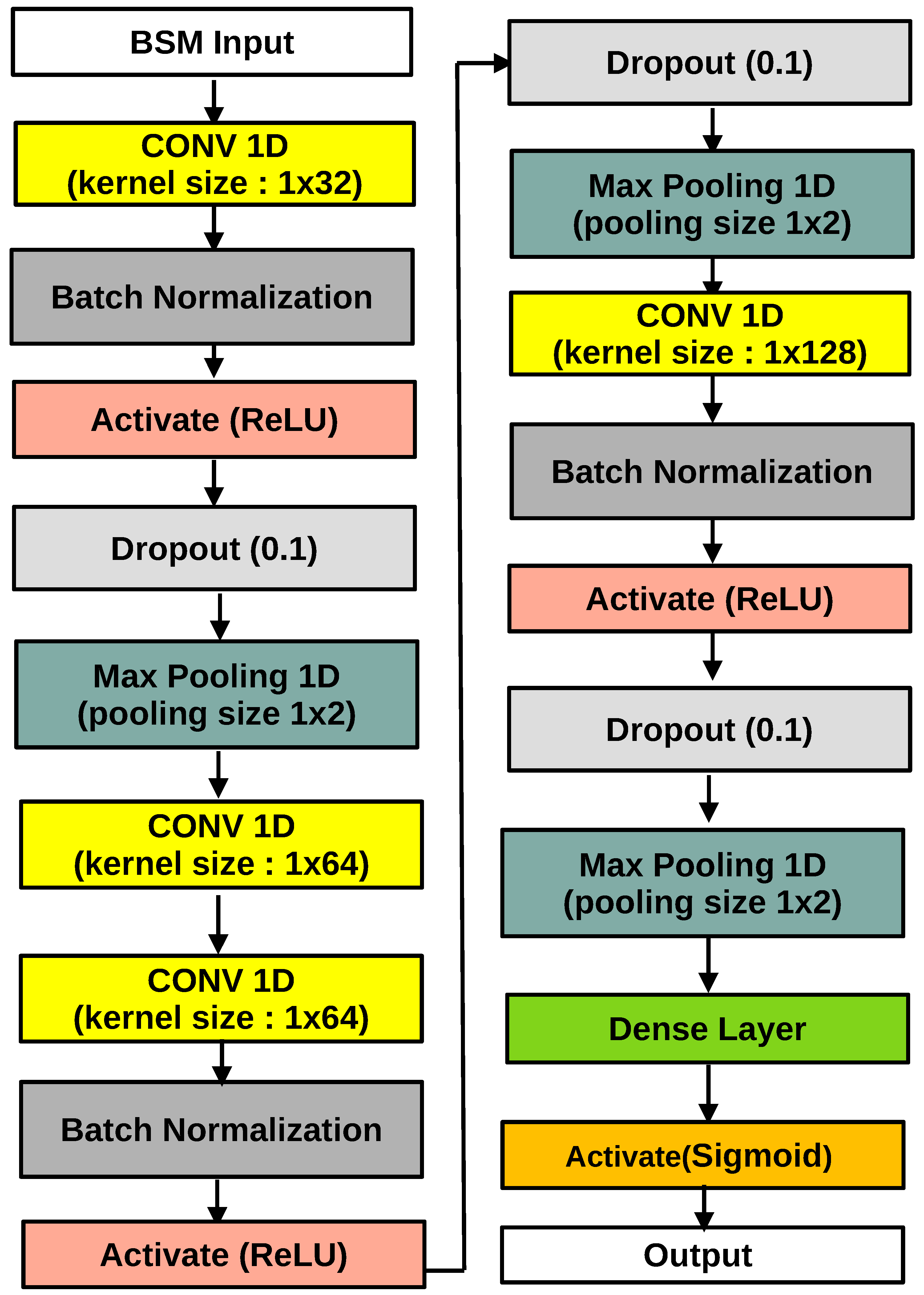
4.1. Convolutional Neural Network (CNN)
Classification Criterion of CNN Algorithm
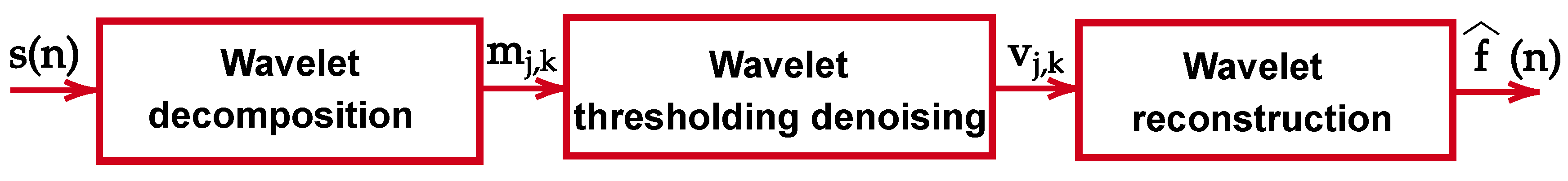
4.2. Discrete Wavelet Transform (DWT)
4.3. Connected and Automated Vehicles (CAVs) Data Characteristics and Anomaly Model
| Algorithm 1: Connected and Automated Vehicles (CAV) Cyber Attack Generation Process. |
|
DWT Pre-Analysis of the Data
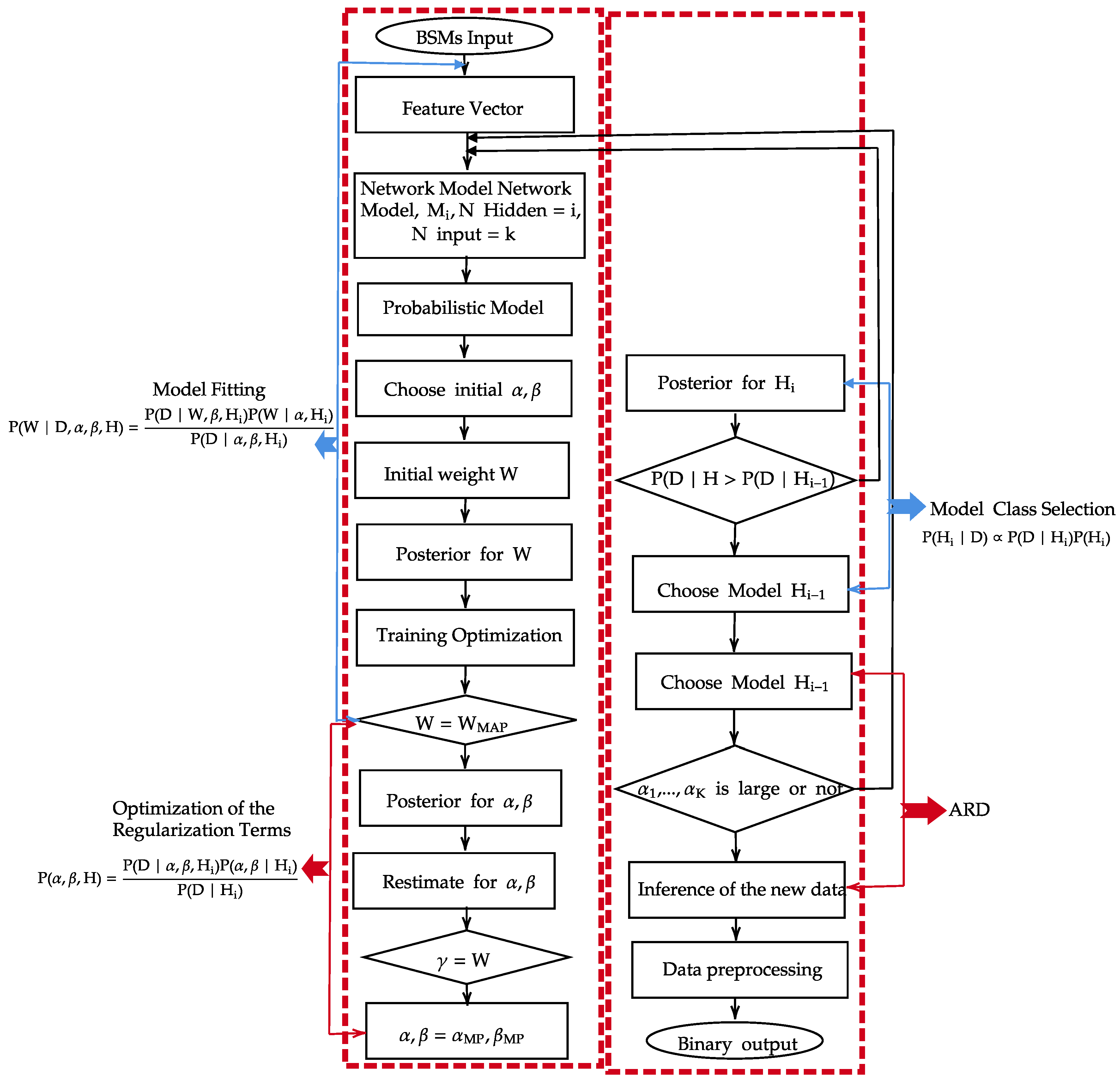
4.4. Bayesian Deep Learning (BDL)
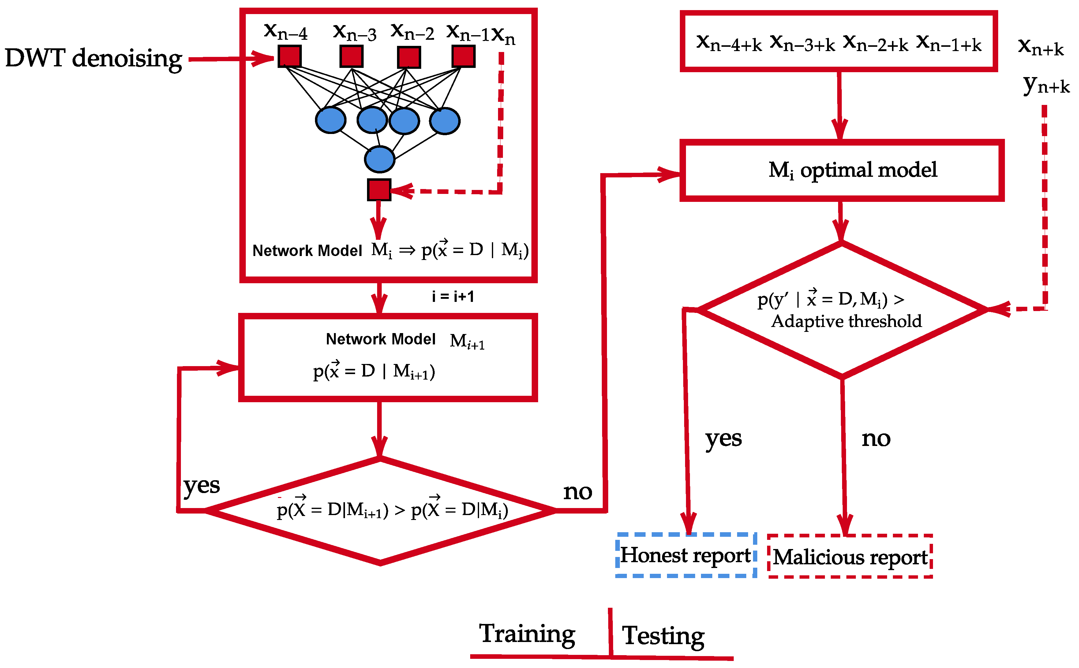
4.5. The Proposed Method
Classification Criterion of the Proposed Approach
5. Results and Discussion
5.1. Mechanisms Under Single Anomaly System
5.1.1. Impact of Network Density on Anomaly Detection
- (i)
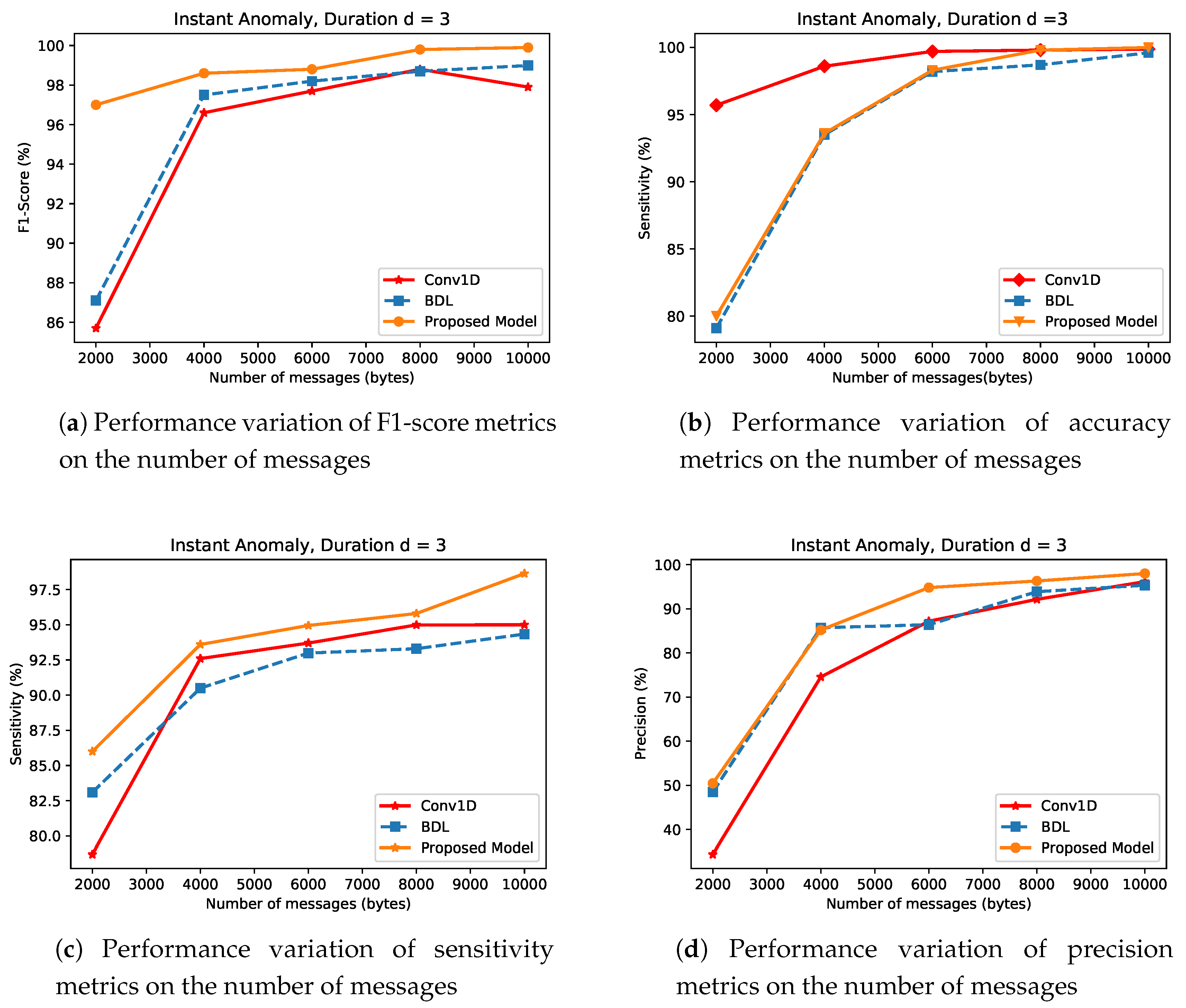
- Instant AnomalyIn this section, the impacts of the magnitude of network density m, on the performance of CNN, BDL and the proposed approach (DWT-BDL) are evaluated. Figure 9 indicates that at a low network density CNN, BDL and the proposed approach show poor performance. This is very much observed in the state-of-the-art approaches compared to the proposed approach. For instance at, m = 2000, CNN and BDL have the performance values of and and and in F1-score as plotted in Figure 9a and sensitivity metrics as plotted in Figure 9c, while the proposed approach improves over CNN and BDL in the same metric values with performance gains of and compared to CNN and and compared to BDL respectively. Similarly, Figure 9d illustrates the superiority of the proposed approach. However, the CNN approach in this scenario maintained a lead performance in some cases of m in the experiment as shown in Figure 9b.However, at high values of m, the overall strength of the detection approaches used in this analysis systematically improves. The proposed approach demonstrates a superior performance over BDL and CNN in all the performance metrics except at some accuracy values as shown in Figure 9b, where CNN has a better performance. However, the proposed approach outperforms CNN, BDL in the rest of the metrics in all the cases of m. For instance, at density m = 10,000, the sensitivity of the proposed approach shows performance gains of and when compared to BDL and CNN, respectively. This superior performance trend of the proposed approach is replicated in all the performance metrics as seen in Figure 9.It can be generalized that as the value of m decreases, the overall detection approaches systematically deteriorates. This clearly indicates the relevance of m in anomaly detection system. The consistent superior performances of the proposed approach, relatively in all the metrics as a result of combining the performance of the BDL and DWT. The proposed approach utilizes the decomposition and denoising qualities of DWT, coupled with the robust BDL mechanism in optimal decision making.
- (ii)
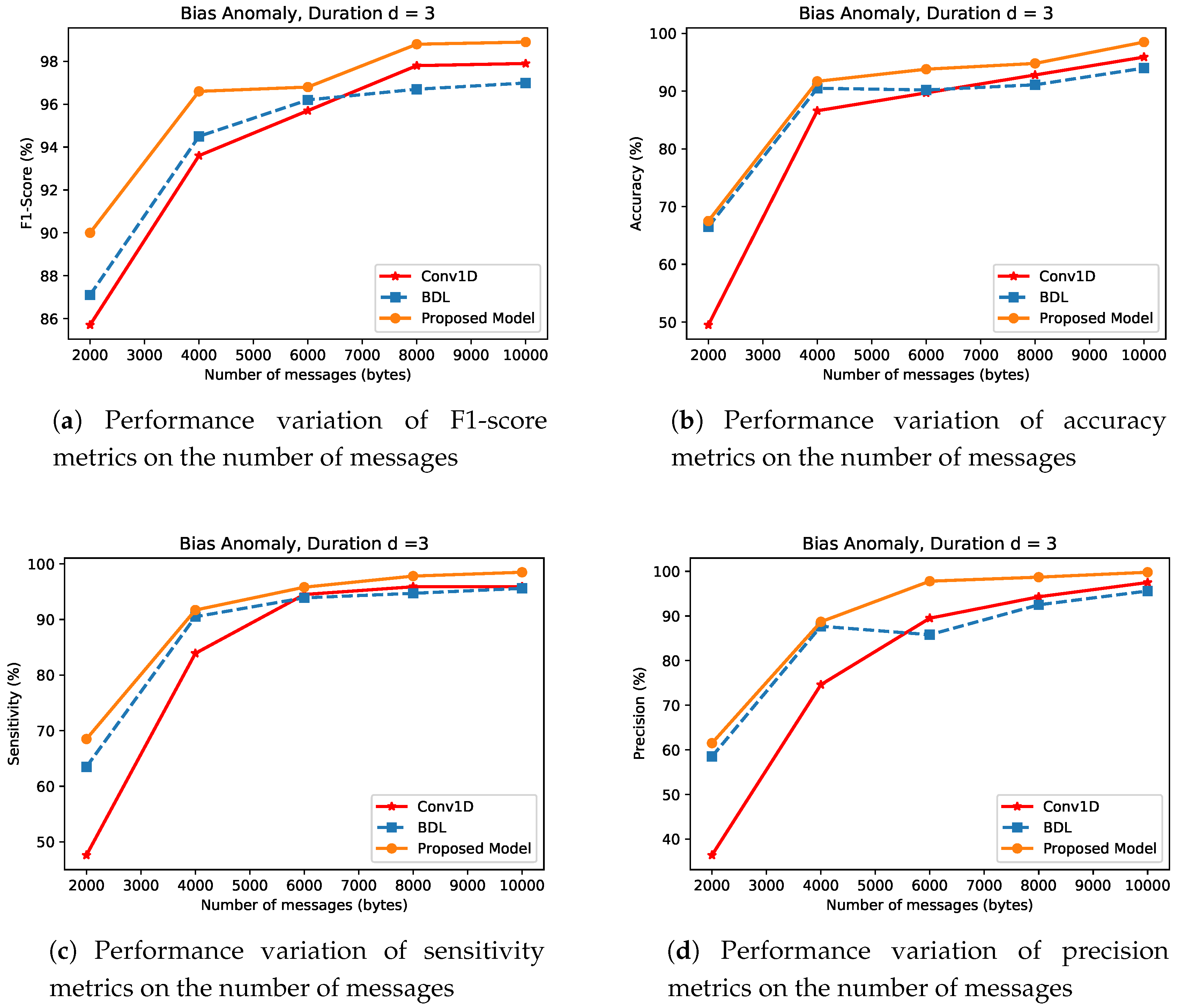
- Bias AnomalyFigure 10 presents the bias anomaly type results for BDL, CNN and the proposed mechanism. As demonstrated in the experiments, at a very small magnitude of m, the BDL approach performs better than the CNN, while the proposed approach outperforms both BDL and CNN mechanisms in all the metrics in small network density scenario. For example, BDL’s accuracy as shown in Figure 10b, by approximately higher than CNN’s, while the proposed approach has performance gain of and over BDL and CNN respectively, with m = 2000 samples drawn from .At m = 10,000 in the simulation, the efficiency of these approaches increase as the magnitude of network density increases. Detection mechanisms in this anomaly/attack case show a similar behavior as shown in instant anomaly case with the distribution drawn from a fixed random variable and duration . The proposed approach shows improvement in sensitivity metrics as illustrated in Figure 10c, more than BDL and CNN by values of and , respectively. Similarly, the performance evaluation on bias anomaly as demonstrated in Figure 10a,d support the superiority of the proposed approach over BDL and CNN.
- (iii)
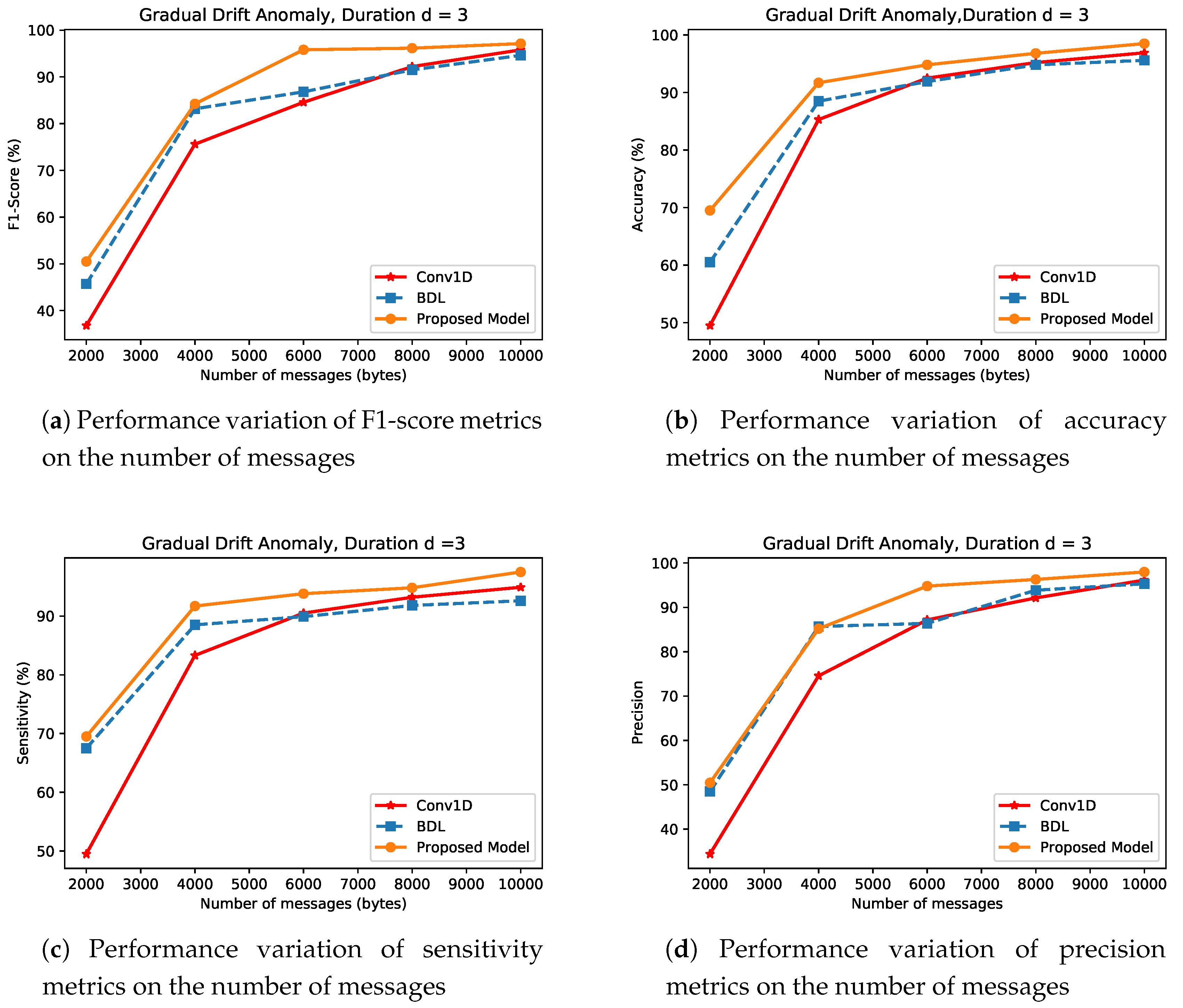
- Gradual Drift AnomalyFigure 11 shows the results of the BDL, CNN, and proposed approach for gradual drift anomaly type detection. This type of anomaly involves a gradual rise in sensor values making it difficult to identify and discern the onset of anomaly from normal sensor values. In general, for a small magnitude of network densities, BDL outperforms the CNN detection performance. For instance, in Figure 11a,d using BDL approach, at network density of 2000, the F1-score and precision respectively, increase by approximately and when compared to CNN mechanism. However, at high magnitude of network density, CNN consistently outperforms BDL in all the performance across the experiments. For instance, at m = 10,000, the F1-score and precision metrics of CNN, improve by and over BDL approach.Considering the anomaly detection performance of the proposed approach for gradual drift anomaly, the following is noted. The experiments indicate that the proposed approach provides a significant improvement in low and high density networks scenarios when compared to CNN and BDL. For instance, at low density network, the proposed approach in respect to F1-score, precision and sensitivity, as plotted in Figure 11a,c,d has performance gains of , and , respectively, over CNN approach and , and compared to BDL. At a high value of m, the detection performance of the various approaches used in this context increase across all the metrics. Furthermore, it is shown that in general, the proposed approach outperforms CNN and BDL. For instance, experiment carried out on network density of 10,000, again shows that F1-score, precision and sensitivity approach are increased by , and over the CNN mechanism, and by , and over BDL approach. Moreover, the proposed approach improves upon the detection performance of both DWT and BDL respectively.
Discussions of the Mechanisms Under Single Anomaly
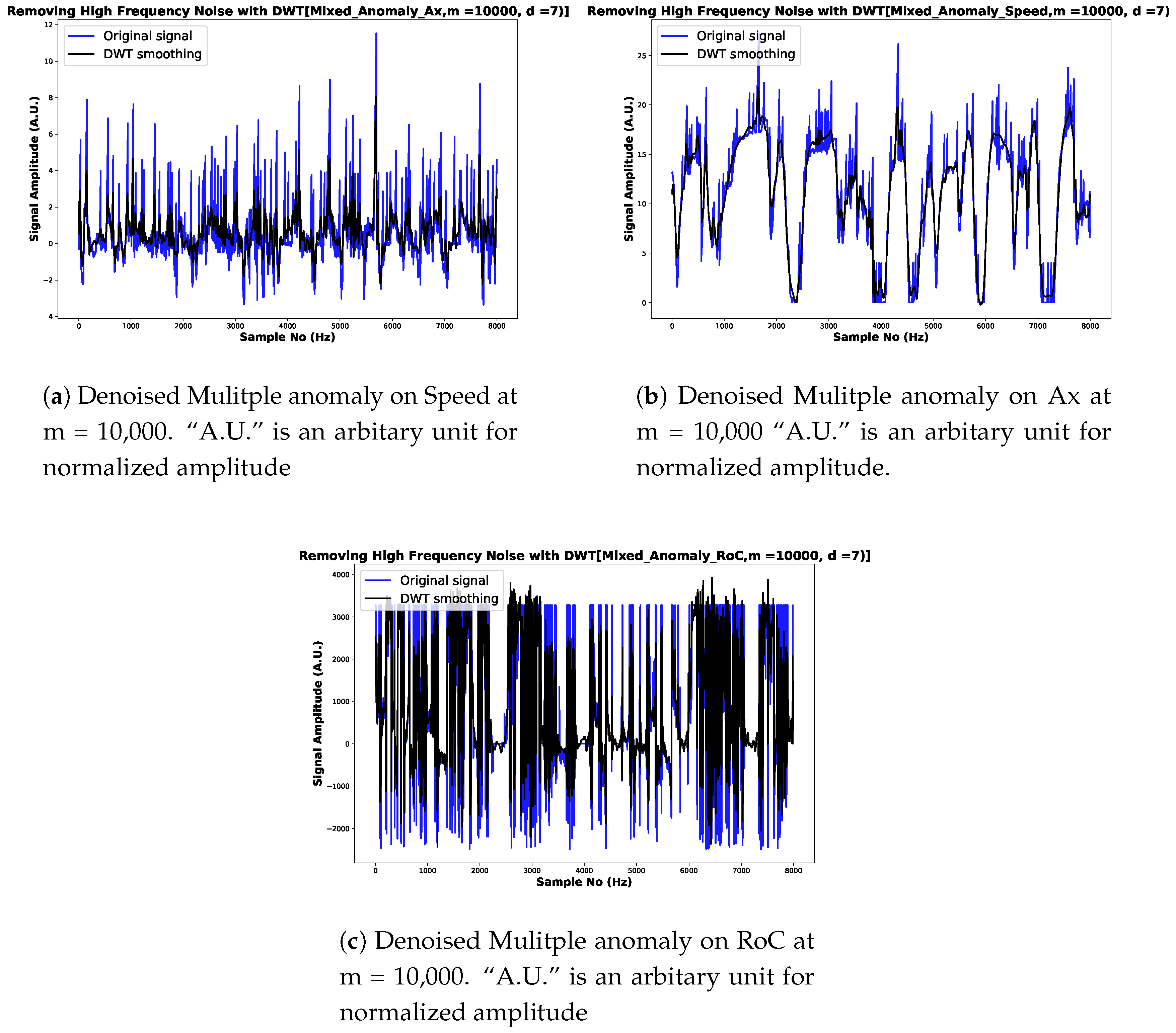
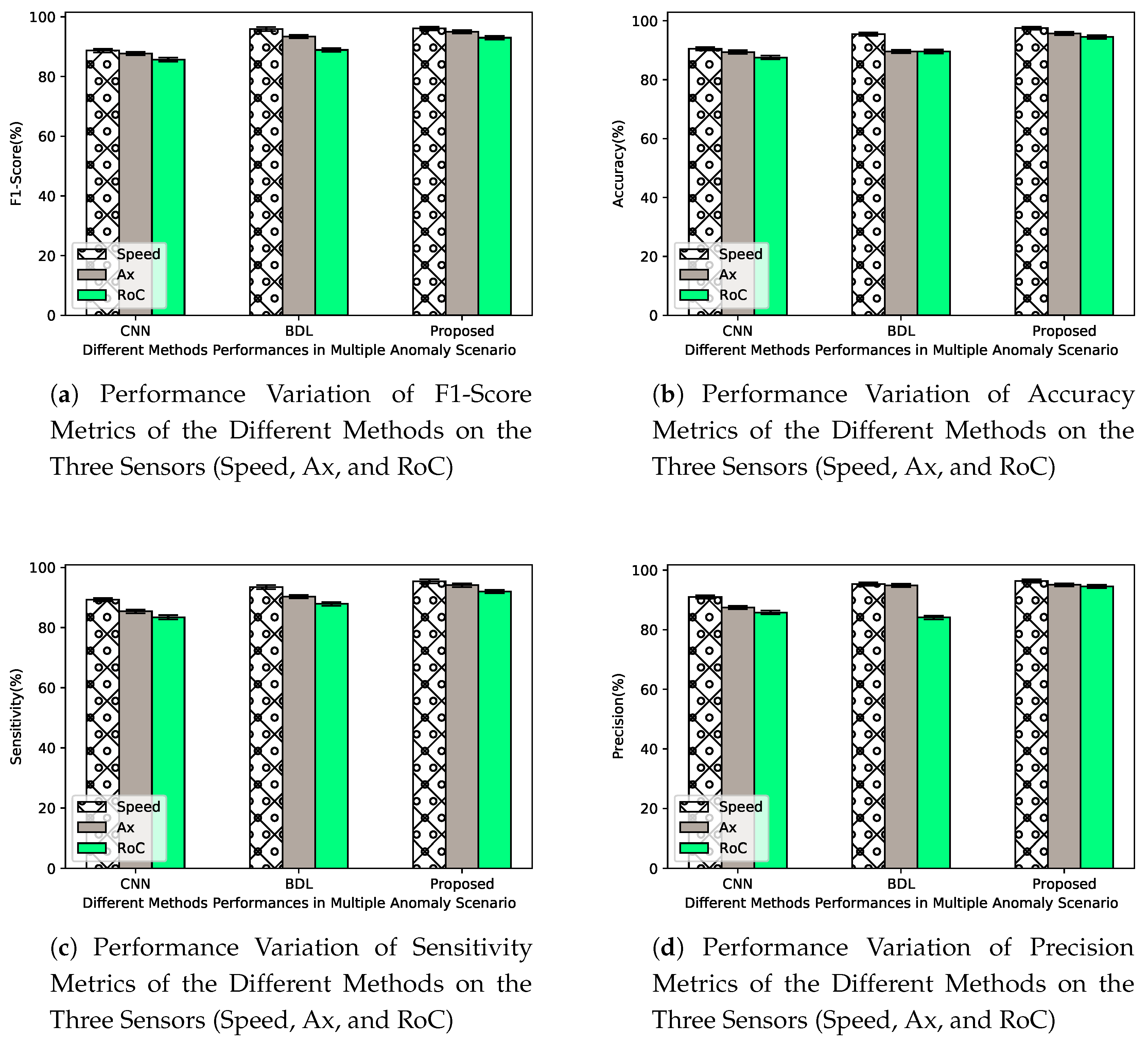
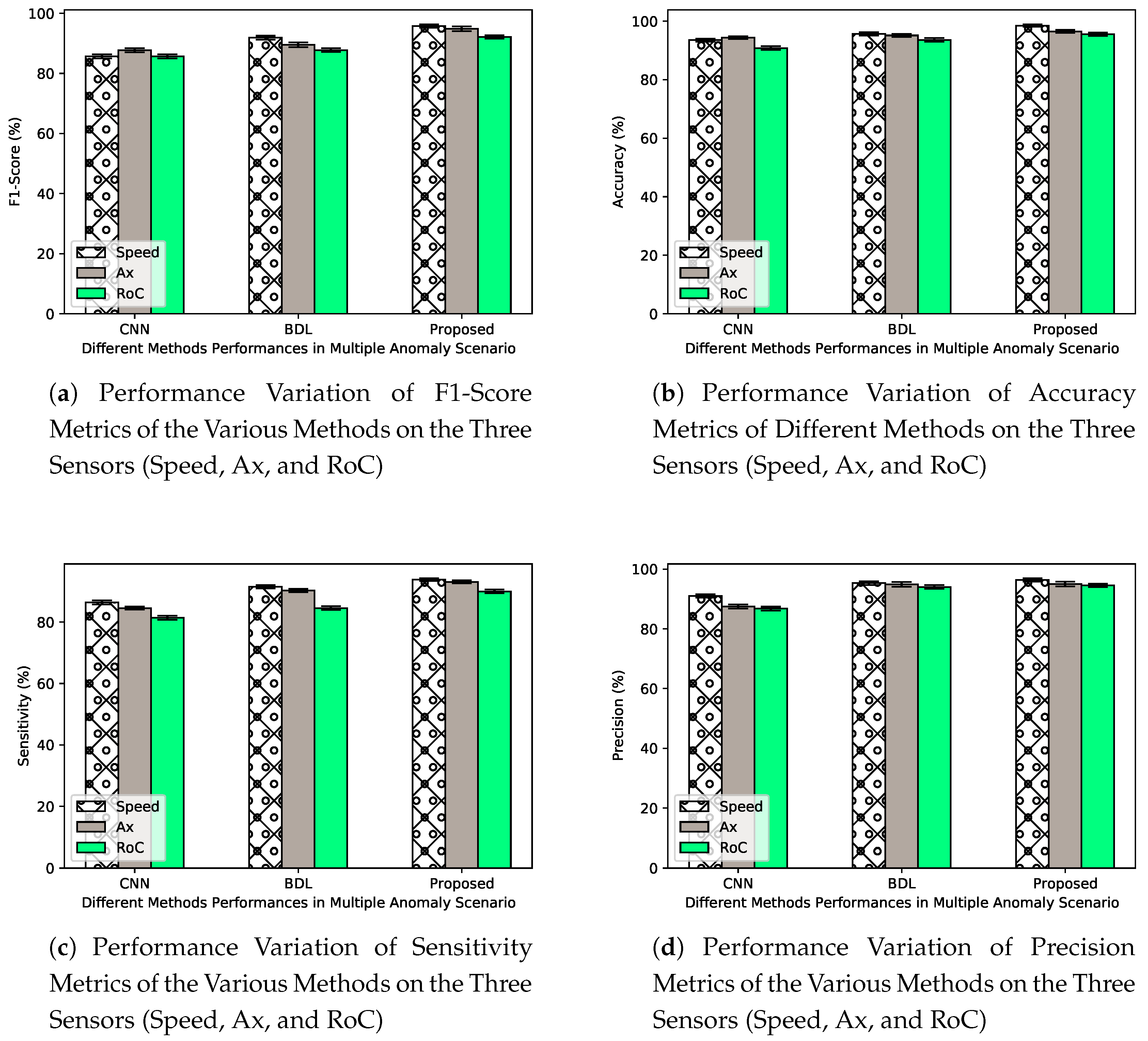
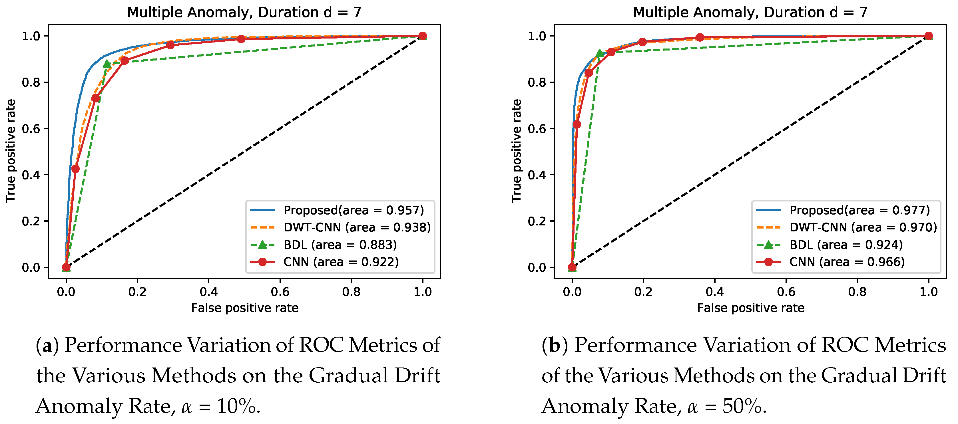
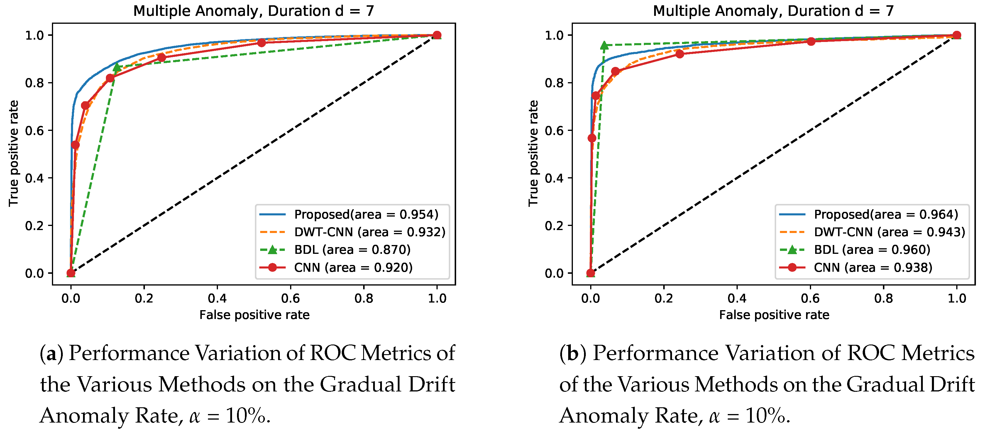
5.2. Mechanisms Under Multiple Anomaly System
Discussion of the Mechanisms Under Multiple Anomaly
6. Conclusions
Author Contributions
Funding
Acknowledgments
Conflicts of Interest
References
- Ahmed, S.; Tepe, K. Entropy-Based Recommendation Trust Model for Machine to Machine Communications. In Ad Hoc Networks; Springer: Berlin, Germany, 2017; pp. 297–305. [Google Scholar]
- Grace, N.; Thornton, P.; Johnson, J.; Blythe, K.; Oxley, C.; Merrefield, C.; Bartinique, I.; Morin, D.; Zhang, R.; Johnson-Moffet, L.; et al. Volpe Center Annual Accomplishments: Advancing Transportation Innovation for the Public Good—January 2018; Technical Report; National Transportation Systems Center (US): Cambridge, MA, USA, 2018.
- Den Hartog, J.; Zannone, N. Security and privacy for innovative automotive applications: A survey. Comput. Commun. 2018, 132, 17–41. [Google Scholar]
- Ahmed, S. Trust Establishment and Management in Adhoc Networks. Ph.D. Thesis, University of Windsor, Windsor, ON, Canada, 16 September 2016. [Google Scholar]
- Liu, J.; Khattak, A.J. Delivering improved alerts, warnings, and control assistance using basic safety messages transmitted between connected vehicles. Transp. Res. Part C Emerg. Technol. 2016, 68, 83–100. [Google Scholar] [CrossRef]
- Cai, R.; Zhang, Z.; Tung, A.K.; Dai, C.; Hao, Z. A general framework of hierarchical clustering and its applications. Inf. Sci. 2014, 272, 29–48. [Google Scholar] [CrossRef]
- Wang, Y.; Masoud, N.; Khojandi, A. Real-Time Sensor Anomaly Detection and Recovery in Connected Automated Vehicle Sensors. IEEE Trans. Intell. Transp. Syst. 2020. [Google Scholar] [CrossRef]
- Van Wyk, F.; Wang, Y.; Khojandi, A.; Masoud, N. Real-time sensor anomaly detection and identification in automated vehicles. IEEE Trans. Intell. Transp. Syst. 2019, 21, 1264–1276. [Google Scholar] [CrossRef]
- Ahmad, S.; Lavin, A.; Purdy, S.; Agha, Z. Unsupervised real-time anomaly detection for streaming data. Neurocomputing 2017, 262, 134–147. [Google Scholar] [CrossRef]
- Petit, J.; Feiri, M.; Kargl, F. Spoofed data detection in vanets using dynamic thresholds. In Proceedings of the 2011 IEEE Vehicular Networking Conference (VNC), Amsterdam, The Netherlands, 14–16 November 2011; pp. 25–32. [Google Scholar]
- Checkoway, S.; McCoy, D.; Kantor, B.; Anderson, D.; Shacham, H.; Savage, S.; Koscher, K.; Czeskis, A.; Roesner, F.; Kohno, T.; et al. Comprehensive experimental analyses of automotive attack surfaces. In Proceedings of the USENIX Security Symposium, San Francisco, CA, USA, 8–12 August 2011; Volume 4, pp. 447–462. [Google Scholar]
- Weimerskirch, A.; Gaynier, R. An Overview of Automotive Cybersecurity: Challenges and Solution Approaches. In Proceedings of the 5th International Workshop on Trustworthy Embedded Devices Co-Located with CCS 2015, University of Michigan, Ann Arbor, MI, USA, 16 September 2015; p. 53. [Google Scholar]
- Salahshoor, K.; Mosallaei, M.; Bayat, M. Centralized and decentralized process and sensor fault monitoring using data fusion based on adaptive extended Kalman filter algorithm. Measurement 2008, 41, 1059–1076. [Google Scholar] [CrossRef]
- Sewak, M.; Singh, S. IoT and distributed machine learning powered optimal state recommender solution. In Proceedings of the 2016 International Conference on Internet of Things and Applications (IOTA), Pune, India, 22–24 January 2016; pp. 101–106. [Google Scholar]
- Petit, J.; Shladover, S.E. Potential cyberattacks on automated vehicles. IEEE Trans. Intell. Transp. Syst. 2014, 16, 546–556. [Google Scholar] [CrossRef]
- Müter, M.; Asaj, N. Entropy-based anomaly detection for in-vehicle networks. In Proceedings of the 2011 IEEE Intelligent Vehicles Symposium (IV), Baden-Baden, Germany, 5–9 June 2011; pp. 1110–1115. [Google Scholar]
- Marchetti, M.; Stabili, D.; Guido, A.; Colajanni, M. Evaluation of anomaly detection for in-vehicle networks through information-theoretic algorithms. In Proceedings of the 2016 IEEE 2nd International Forum on Research and Technologies for Society and Industry Leveraging a Better Tomorrow (RTSI), Bologna, Italy, 7–9 September 2016; pp. 1–6. [Google Scholar]
- Ding, D.; Han, Q.L.; Xiang, Y.; Ge, X.; Zhang, X.M. A survey on security control and attack detection for industrial cyber-physical systems. Neurocomputing 2018, 275, 1674–1683. [Google Scholar] [CrossRef]
- Van der Heijden, R.W.; Lukaseder, T.; Kargl, F. Veremi: A dataset for comparable evaluation of misbehavior detection in vanets. In Proceedings of the International Conference on Security and Privacy in Communication Systems, Singapore, 8–10 August 2018; pp. 318–337. [Google Scholar]
- Škorić, B.; de Hoogh, S.J.; Zannone, N. Flow-based reputation with uncertainty: Evidence-based subjective logic. Int. J. Inf. Secur. 2016, 15, 381–402. [Google Scholar] [CrossRef]
- Eziama, E.; Tepe, K.; Balador, A.; Nwizege, K.S.; Jaimes, L.M. Malicious Node Detection in Vehicular Ad-Hoc Network Using Machine Learning and Deep Learning. In Proceedings of the 2018 IEEE Globecom Workshops (GC Wkshps), Abu Dhabi, UAE, 21 February 2018; pp. 1–6. [Google Scholar]
- Godsmark, P.; Kirk, B.; Gill, V.; Flemming, B. Automated Vehicles: The Coming of the Next Disruptive Technology; The Van Horne Institute: Calgary, AB, Canada, 22 January 2016. [Google Scholar]
- Yang, Y.; Feng, Q.; Sun, Y.L.; Dai, Y. RepTrap: A novel attack on feedback-based reputation systems. In Proceedings of the 4th International Conference on Security and Privacy in Communication Netowrks, Istanbul, Turkey, 22 September 2008; p. 8. [Google Scholar]
- Ozay, M.; Esnaola, I.; Vural, F.T.Y.; Kulkarni, S.R.; Poor, H.V. Machine learning methods for attack detection in the smart grid. IEEE Trans. Neural Netw. Learn. Syst. 2015, 27, 1773–1786. [Google Scholar] [CrossRef]
- Petrillo, A.; Pescape, A.; Santini, S. A secure adaptive control for cooperative driving of autonomous connected vehicles in the presence of heterogeneous communication delays and cyberattacks. IEEE Trans. Cybern. 2020. [Google Scholar] [CrossRef]
- Liu, X.; Datta, A.; Lim, E.P. Computational Trust Models and Machine Learning; CRC Press: Boca Raton, FL, USA, 2014. [Google Scholar]
- Zaidi, K.; Milojevic, M.B.; Rakocevic, V.; Nallanathan, A.; Rajarajan, M. Host-based intrusion detection for vanets: A statistical approach to rogue node detection. IEEE Trans. Veh. Technol. 2015, 65, 6703–6714. [Google Scholar] [CrossRef]
- Ahmed, S.; Al-Rubeaai, S.; Tepe, K. Novel Trust Framework for Vehicular Networks. IEEE Trans. Veh. Technol. 2017, 66, 9498–9511. [Google Scholar] [CrossRef]
- Zhang, H.; Huang, L.; Wu, C.Q.; Li, Z. An Effective Convolutional Neural Network Based on SMOTE and Gaussian Mixture Model for Intrusion Detection in Imbalanced Dataset. Comput. Netw. 2020, 177, 107315. [Google Scholar] [CrossRef]
- Li, M.; Wang, Z.; Luo, J.; Liu, Y.; Cai, S. Wavelet denoising of vehicle platform vibration signal based on threshold neural network. Shock Vib. 2017, 2017, 7962828. [Google Scholar] [CrossRef]
- Bezzina, D.; Sayer, J. Safety Pilot Model Deployment: Test Conductor Team Report; USDOT Report No. DOT HS 812 171; United State Department of Transportation: Washington, DC, USA, 2015.
- Bishop, C.M. Neural Networks for Pattern Recognition; Oxford University Press: Oxford, UK, 1995. [Google Scholar]
- Arangio, S.; Beck, J. Bayesian neural networks for bridge integrity assessment. Struct. Control Health Monit. 2012, 19, 3–21. [Google Scholar] [CrossRef]
- Gal, Y. Uncertainty in Deep Learning; University of Cambridge: Cambridge, UK, 2016. [Google Scholar]
- Ghahramani, Z. A history of bayesian neural networks. In Proceedings of the NIPS Workshop on Bayesian Deep Learning, Bercelona, Spain, 10 December 2016. [Google Scholar]
- Rodrigo, H.S. Bayesian Artificial Neural Networks in Health and Cybersecurity. Ph.D. Thesis, University of South Florida, Tempa, FL, USA, 2017. [Google Scholar]
- Raya, M.; Papadimitratos, P.; Gligor, V.D.; Hubaux, J.P. On data-centric trust establishment in ephemeral ad hoc networks. In Proceedings of the IEEE INFOCOM 2008—The 27th Conference on Computer Communications, Phoenix, AZ, USA, 13–18 April 2008; pp. 1238–1246. [Google Scholar]
- Goh, S.T. Machine Learning Approaches to Challenging Problems: Interpretable Imbalanced Classification, Interpretable Density Estimation, and Causal Inference. Ph.D. Thesis, Massachusetts Institute of Technology, Cambridge, MA, USA, 2018. [Google Scholar]
- Koyejo, O.O.; Natarajan, N.; Ravikumar, P.K.; Dhillon, I.S. Consistent binary classification with generalized performance metrics. In Proceedings of the Neural Information Processing Systems Conference (NIPS 2014), Montréal, QC, Canada, 8–13 December 2014; pp. 2744–2752. [Google Scholar]
- Silvestro, D.; Andermann, T. Prior choice affects ability of Bayesian neural networks to identify unknowns. arXiv 2020, arXiv:2005.04987. [Google Scholar]
- Maier, A.; Lorch, B.; Riess, C. Toward Reliable Models for Authenticating Multimedia Content: Detecting Resampling Artifacts With Bayesian Neural Networks. arXiv 2020, arXiv:2007.14132. [Google Scholar]


| Instant Anomaly (Network Size m) | (Anomaly) | (Anomaly) | (Wavelet dB(12)) | (Wavelet dB(12)) |
| 2000 | 10.307401 | 6.170231 | 10.300251 | 5.7634621 |
| 4000 | 10.307407 | 6.170261 | 10.300258 | 5.763563 |
| 6000 | 10.307414 | 6.170258 | 10.300262 | 5.7635907 |
| 8000 | 10.307417 | 6.1702566 | 10.300263 | 5.7635937 |
| 10,000 | 10.307415 | 6.170257 | 10.300264 | 5.7635903 |
| Bias Anomaly (Network Size m) | (Anomaly) | (Anomaly) | (Wavelet dB(12)) | (Wavelet dB(12)) |
| 2000 | 0.5829332 | 1.5610949 | 0.5813745 | 1.1946311 |
| 4000 | 0.53638434 | 1.581967 | 0.53705674 | 1.0952997 |
| 6000 | 0.6300388 | 1.7301117 | 0.6321792 | 1.0724595 |
| 8000 | 0.64839834 | 1.6975222 | 0.65079004 | 1.0431184 |
| 10,000 | 0.7417457 | 1.7784712 | 0.74250895 | 1.0478663 |
| Gradual Drift Anomaly (Network Size m) | (Anomaly) | (Anomaly) | (Wavelet dB(12)) | (Wavelet dB(12)) |
| 2000 | 0.07693122 | 0.910007 | 0.076246604 | 0.4898912 |
| 4000 | 0.07699456 | 0.9098382 | 0.0763265 | 0.49061427 |
| 6000 | 0.07699457 | 0.908578 | 0.07632571 | 0.49055964 |
| 8000 | 0.07699094 | 0.9098535 | 0.07632209 | 0.49055964 |
| 10,000 | 0.07699085 | 0.9098535 | 0.07632202 | 0.49055642 |
Publisher’s Note: MDPI stays neutral with regard to jurisdictional claims in published maps and institutional affiliations. |
© 2020 by the authors. Licensee MDPI, Basel, Switzerland. This article is an open access article distributed under the terms and conditions of the Creative Commons Attribution (CC BY) license (http://creativecommons.org/licenses/by/4.0/).
Share and Cite
Eziama, E.; Awin, F.; Ahmed, S.; Marina Santos-Jaimes, L.; Pelumi, A.; Corral-De-Witt, D. Detection and Identification of Malicious Cyber-Attacks in Connected and Automated Vehicles’ Real-Time Sensors. Appl. Sci. 2020, 10, 7833. https://doi.org/10.3390/app10217833
Eziama E, Awin F, Ahmed S, Marina Santos-Jaimes L, Pelumi A, Corral-De-Witt D. Detection and Identification of Malicious Cyber-Attacks in Connected and Automated Vehicles’ Real-Time Sensors. Applied Sciences. 2020; 10(21):7833. https://doi.org/10.3390/app10217833
Chicago/Turabian StyleEziama, Elvin, Faroq Awin, Sabbir Ahmed, Luz Marina Santos-Jaimes, Akinyemi Pelumi, and Danilo Corral-De-Witt. 2020. "Detection and Identification of Malicious Cyber-Attacks in Connected and Automated Vehicles’ Real-Time Sensors" Applied Sciences 10, no. 21: 7833. https://doi.org/10.3390/app10217833
APA StyleEziama, E., Awin, F., Ahmed, S., Marina Santos-Jaimes, L., Pelumi, A., & Corral-De-Witt, D. (2020). Detection and Identification of Malicious Cyber-Attacks in Connected and Automated Vehicles’ Real-Time Sensors. Applied Sciences, 10(21), 7833. https://doi.org/10.3390/app10217833