Abstract
In the past three decades, ultrafast pulse laser technology has greatly progressed and applied widely in many subjects, such as physics, chemistry, biology, materials, and so on. Accordingly, as well as for future developments, to measure or characterize the pulses temporally in femtosecond domain is indispensable but still challenging. Based on the operation principles, the measurement techniques can be classified into three categories: correlation, spectrogram, and spectral interferometry, which operate in time-domain, time-frequency combination, and frequency-domain, respectively. Here, we present a mini-review for these techniques, including their operating principles, development status, characteristics, and challenges.
1. Introduction
Since the 1990s, ultrashort pulse laser technology has greatly progressed. Nowadays, the peak power of laser pulse reaches up to PW [1], the intensity goes beyond 1022 W/cm2 [2,3], while the pulse width can be controlled at few-cycle even sub-cycle of light [4]. Simultaneously, ultrashort pulse lasers are widely applied in many subjects, such as physics, chemistry, biology, medicine, materials, and so on. Correspondingly, characterizing temporally laser pulse becomes more and more important no matter for the developments of ultrafast laser technology or its applications. To measure a transient physical quantity, we need another controllable faster quantity as a “time ruler” to compare with it. For example, in a streak camera [5], the time ruler is the electric-field gradient in the picosecond scale. However, ultrashort laser pulses in the femtosecond scale are so fast that it is difficult to arrange their ruler except themselves. So practically, characterizing ultrashort pulses usually works by “light measures light”, or by the comparison between a test pulse and a reference pulse. The reference can be the frequency-conversion [6], or spectral modulation [7,8] from the test pulse, as well as the test pulse itself [9]. Spectral interference [7,8] or optical nonlinearity [9] is induced for the comparison between the test and the reference. The measurement can be carried out in the time-domain [6,10], frequency-domain [7,8], or both [11,12]. In the time-domain, the most important parameter is the delay time between the test and the reference, which is controlled by their fly-time difference in the light paths. In the frequency-domain, spectrograph can be directly applied to spectral measurements for the output light, which benefits from the wide bandwidth of the ultrashort pulses. In the ultrashort pulse measurement, optical nonlinearity, as an all-rounder, e.g., frequency-conversion, correlation, spectral convolution, or time-filtering [6,7,8,9,10,11,12,13], plays a very important role.
In this article, we review the developments of the technologies to measure ultrashort light pulses in recent years, which divides into three types: correlation [6,10], spectrogram [11,12], and spectral interferometry [7,8], which are based on time-domain, time-frequency combining, and frequency-domain measurements, respectively. Correlation is a simple, robust, and high signal-to-noise ratio (SNR) method to obtain the pulse intensity information but without the phase information. It is not suitable for characterizing pulses with complicated structures, e.g., asymmetric airy pulses [14], white-light supercontinuum [15]. Spectrogram and spectral interferometry can measure the complete information of the pulse with both intensity and phase. Spectrogram usually can be seen as a frequency-resolved correlation measurement, light field information is retrieved from the 2-dimension (2D) time-frequency spectrogram by an iterative algorithm. Spectral Interferometry is based on direct spectral phase measurement by self-reference interferometry. All the three techniques have their single-shot versions which are suitable for pulses those with low repetitive rate. The article is arranged as follows: Section 2 shows the basics of the ultrashort laser pulse; Section 3, Section 4 and Section 5 introduce the techniques based on correlation, spectrogram, and spectral interferometry, respectively; Section 6 is the Conclusion and Prospects.
2. The Basics
For the sake of simplicity, we consider the electric field of the laser pulse as a linearly polarized plane wave, so we can write it in scalar form without space coordinates [12]
where t is time in the reference frame of the pulse, ω0 is the carrier angular frequency, I(t) and ϕ(t) are the time-dependent intensity and phase, c.c. means complex conjugate. Except where otherwise stated, we use its complex form in this article for convenience: ε(t) = 1/2I(t)0.5 exp[iω0t − iϕ(t)]. Here, both I(t) and exp[iϕ(t)] usually vary much slower than the carrier term exp(iω0t). In laser pulse measurement, we usually ignore the carrier term and use electric field complex amplitude to describe the laser pulse:
εR(t) = 1/2I(t)0.5 exp[iω0t − iϕ(t)] + c.c.
E(t) = I(t)0.5 exp[−iϕ(t)].
In the frequency domain, the spectrum of the electric field is the Fourier transform of ε(t): ε(ω) = ∫ε(t)exp(−iω’t)dt = E(ω’ − ω0), which means that the spectrum structure of the pulse is decided by its amplitude. Separating E(ω’ − ω0) into its intensity and phase and let ω = ω’ − ω0 which is the relative frequency around the carrier frequency, yields
E(ω) = S(ω)0.5 exp[−iφ(ω)].
Equations (2) and (3) are the equivalent descriptions for a laser pulse. In these two sets of parameters {I(t), ϕ(t)} and {S(ω), φ(ω)}, if we know one, another is easy to obtain by applying Fourier transform. Only S(ω) can be measured by a spectrometer directly, so the restoring of E(t) or ε(t) is turned into the question of reconstructing φ(ω). We can write a Taylor series for spectral phase φ(ω) = φ0 + φ1ω + φ2ω2/2 + φ3ω3/6 + ... [16]. The zeroth-order term is the absolute phase, the first-order term shifts the pulse in time without changing the shape, the second-order term induces a linear chirp, and the third-order term causes an asymmetric structure to the pulse [14]. The zero and first orders of the phase do not impact the shape of the pulse and can be ignored in measurement, what we take care of is the high-order terms. Correlation method measures or estimates I(t) in time-domain. A typical spectrogram method Frequency-Resolved Optical Gating (FROG) [11,12], measures the information of the combine of I(t) and S(ω) for “piecing together” φ(ω). Spectral interferometry, e.g., Spectral Phase Interferometry for Direct Electric-field Reconstruction (SPIDER) [7,8], measures the spectral phase φ(ω) directly.
3. Correlation Measurement
Correlation is a technique to estimate the pulse intensity I(t) in time-domain without obtaining the phase information, so it does not implement a complete measurement. However, correlation is irreplaceable for its simple, robust, and ultrahigh signal-to-noise ratio (SNR). The simplest correlator, called field-autocorrelator (or linear autocorrelator), is composed of a Michelson interferometer (MI) and an integrating detector. It operates in the time domain, and the acquiring signal is Γ(2)(τ) = ∫E(t)E*(t − τ)dt when neglecting the constant term, where τ is the delay between two pulses from two arms in MI. The Fourier transform of Γ(2) is just the spectrum S(ω) of the test pulse, so the field-autocorrelator can also work as a Fourier-transform spectrometer [17,18] which cannot give us the time information of the pulse. An effective method to give us the time information of the femtosecond pulses is intensity-autocorrelator, for which we only need to make a minor alter to the field-autocorrelator, by introducing a nonlinear crystal before the detector for second-harmonic generation (SHG). For convenience, when we mention autocorrelator later in the article, it means intensity-autocorrelator. The measured signal is expressed as
and its intensity is related to the temporal overlap of the pulse replicas, so autocorrelation can reflect the pulse length. It is easy to see A(2)(τ) is an even function and symmetric with τ = 0. However, because the probe and the test pulse are divided from the same pulses, A(2)(τ) is not an accurate method to describe, because it is affected by the pulse shapes. The correction factors between pulse-widths to A(2)(τ)-widths, called the deconvolution factor, are given in Ref. [19]. Autocorrelator can realize measurement in single-shot based on space-time correlation of tilt incidence pulses, i.e., time-to-space encoding. If we use a collinear design for Autocorrelator, the sum-frequency (SF) term superposes with the self-frequency-doubling terms, the output signal is
which gives an autocorrelation signal with interferometric fringes [20,21], called interferometric autocorrelation. From the structure of fringes, the chirp of the pulse can be estimated. Nowadays, autocorrelation is a proven technique, and have been applied widely due to its simplicity and cost-of-effectivity. It has been realized with many commercial versions [22,23,24], based on single-shot or scanning, with a wavelength from 200 nm to 12 μm, pulse widths from sub-10 fs to 500 ps, using a photodiode detector, photomultiplier, or two-photon detector as the detector.
A(2)(τ) = ∫I(t)I(t − τ)dt,
Aint(2)(τ) = ∫|[E(t) + E(t − τ)]2|2dt,
For a laser with peak power higher than terawatt, its contrast, which defines as the ratio of the pulse peak to the peaks of the pre- or post-subpulses, is one of the primary parameters, because the laser is so intense at its focus spot even the pre-subpulses can ionize the target and break the original construction before the main peak comes. The contrast of intense pulse is usually required to be higher than 106 in terawatt laser, even 1010 in petawatt systems [25]. The dynamic range of Spectrogram or Spectral Interferometry methods, based on frequency-resolved measurement, cannot be higher than ~106 [25]. For such high contrast, correlation is the irreplaceable method for its simple and robust structure, and more importantly, the phase-matching requirement of SHG which highly improves the measuring SNR. However, the symmetry of A(2)(τ) limits its applications because it cannot distinguish the pre-subpulses from the post-subpulses. Cross-correlation measures the correlation signal between the test pulse I(t) and a gate pulse Ig(t) which is different from I(t), expressed as
can break the symmetry of the correlation signal. If the gate signal is the harmonic of the test pulse, the cross-correlation is called high-order autocorrelation. For example, third-order autocorrelation [6,10] uses frequency-doubling pulse as the gate pulse, and the signal is written as A(3)(τ) = ∫I(t)I2(t − τ)dt. Scanning cross-correlation, benefiting by the multi-shot measurement, easily realizes high contrast [26,27]. However, the typically reported dynamic range of traditional single-shot cross-correlation is 106–107 [28,29,30]. In 2014, Y. Wang firstly realized a dynamic range higher than 1010 in a 50-ps time window in a single-shot cross-correlator based on time-to-space encoding and fiber-array-based detection. Most recently, a dynamic range of ~1011 within a time window of 65 ps was obtained by using a single-shot four-order autocorrelator, as shown in Figure 1. The gate pulse, generated in a frequency-degenerate four-wave mixing process [31], has the same frequency as the test pulse, which can avoid group-velocity mismatching and realize time resolution up to ~160 fs.
C(2)(τ) = ∫I(t)Ig(t − τ)dt,
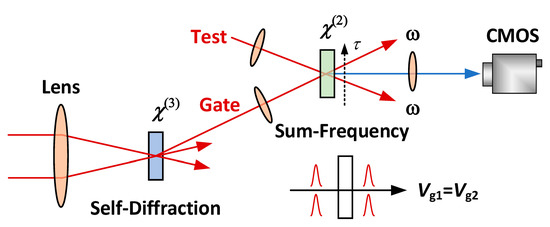
Figure 1.
Schematic of a single-shot four-order autocorrelator. The gate pulse is generated by frequency-degenerate four-wave mixing process.
4. Spectrogram
FROG is a typical method based on spectrogram measurement [32], where the recorded trace is
where g(t − τ) is the gate function with a delay τ relative to the test field E(t). FROG can also be seen as a frequency-resolved correlation. D. Kane and R. Trebino [11] pointed out that the problem of inverting the FROG trace is equivalent to the two-dimensional phase-retrieval problem [33], which can yield essentially unique results, compared to the unsolvable one-dimensional phase-retrieval. In FROG, the input pulse is divided into two parts, one is the test pulse, the other is used to generate an ultrafast time gate that is induced by χ(2)- or χ(3)-nonlinear effects. Many different nonlinear gating mechanisms can be used for FROG, such as polarization-gating (PG) [11], self-diffraction (SD) [34], transient-grating (TG) [35], SHG, third-harmonic generation (THG), and so on. Different versions of FROG generate different kinds of FROG traces and have different strengths and weaknesses. Table 1 shows the comparison of different nonlinearities applied for FROG.

Table 1.
Comparison of different nonlinearities applied for FROG [12,36].
The original version of FROG is a PG-FROG, using time-to-space encoding by cross-incidence, which is designed by D. Kane and R. Trebino [11], as shown in Figure 2. The PG generator is composed of crossed polarizers and a Kerr medium. When the test pulse passes through the PG generator, which is triggered by a delayed pulse, the trace is given by SFROGPG(ω,τ) = |∫E(t)|E(t − τ)|2exp(−iωt) dt|2. Using a cross incident configuration, a single-shot function can be gotten for the time-space correlation between test and gate pulses like that in a single-shot autocorrelator.
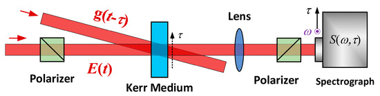
Figure 2.
Schematic of PG-FROG. Time-to-space encoded scanning is caused by cross incidence.
The most common commercial version is SHG-FROG [22,37]. SHG-FROG is a frequency-resolved autocorrelator, so it can be easily realized only by replacing the detector in the autocorrelator with a spectrometer. Another advantage of SHG-FROG’s is its high sensitivity, because it is based on χ(2)-nonlinear effect instead of χ(3)-nonlinear effect used in most other versions of FROG. However, the symmetry of the SHG-FROG traces, like in autocorrelation, brings an ambiguity, or cannot distinguish the sign of the chirp in the measured pulses. To remove this ambiguity, additional steps should be made, such as place a piece of medium in the beam, to introduce a positive chirp. Similar to interferential autocorrelation, SHG-FORG can also operate in a collinear geometry, called interferential FROG, or iFROG [38], to avoid a loss of temporal resolution via geometric effects in the characterization of few-cycle pulses.
FROG works on a 2D spectrograph, so it requires higher energy than those based on spectral interferometry (such as SPIDER), especially when it uses a χ(3)-nonlinear. To improve the sensitivity, cross-correlation FROG (XFROG) was proposed [39]. In an XFROG, the reference pulse is a known pulse that does not need to be spectrally overlapping with the unknow test pulse. The recorded signal is obtained by sum or difference frequency generation of the two pulses. When we use intense reference pulses, this method can be very sensitive. Blue/UV ultrashort pulses or ultrafast fluorescence which is excited by the near-IR pulses are usually very weak. In this case, the intense near-IR pulses are available to serve as a reference pulse using difference-frequency configuration.
Commonly, FROG is expensive relatively and difficult to alignment for the pulse splitting and scanning, phase-matching alignment, and spectral measurement. To simplify FROG, a new version called Grating-eliminated no-nonsense observation of ultrafast incident laser light E-fields (GRENOUILLE) [9] is proposed. As shown in Figure 3, a Fresnel biprism is introduced to replace the beam splitter, delay line, and the beam combiner, a thick crystal is introduced acts as not only the nonlinear medium but also a spectrograph for its angle-independent phase-matching angle and narrow bandwidth. The size of the commercial version is controlled at 26 × 4.5 × 11.5 cm3 [40]. GRENOUILLE is an all-transmission device thus is simple to align and very stable. However, the large thickness of the crystal which required much longer than the group-velocity mismatch length may limit its capability in measuring complex pulse.
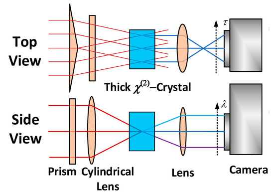
Figure 3.
Schematic of the GRENOUILLE beam geometry. Top view: Time-to-space encoded scanning geometry. Side view: sum-frequency spectrum generation by angle-independent phase-matching.
The trace of FROG can be seen as a joint time-frequency distribution of the pulse, which makes it has some advantages in characterizing complex-pulses compared with autocorrelation or SPIDER that is based on 1D-measurement, such as when applies for “coherent artifact” [41,42]. When multi-shot measurements are made for an unstable, complex pulse train, the autocorrelation trace consists of a narrow spike atop a broad structureless background. The spike, or coherent artifact, reflects the coherent, nonrandom component of the pulse and is usually narrower than the correct pulse length. The broad background indicates the instability, complexity in the pulse train. More important, coherent artifacts may also exist in a pump-probe measurement. M. Rhodes et al. [41] compared several different techniques in measuring unstable pulse trains. The results show that FROGs (SHG-FROG, PG-FROG, and XFROG) perform much better than both Autocorrelator and SPIDER, which only yield coherent artifacts. FROGs retrieve the correct pulse length, distinguish a stable train of short pulses from an unstable train of much longer pulses, benefit by their time-frequency over-determine. PG-FROG and XFROG can even yield the structure roughly.
As mentioned above, 1D phase-retrieval problem is unsolvable, to obtain the spectral phase, FROG introduces a delay scanning dimension τ in spectral measurement, to construct a solvable 2D spectrogram S(ω,τ). Here, τ is not irreplaceable. If appropriately replace τ with another parameter ξ, we may construct another solvable trace S(ω,ξ), we call this trace generalized spectrogram. Nowadays, some generalized spectrogram methods are proposed, such as Multiphoton intrapulse interference phase scan (MIIPS) [43,44,45,46], dispersion scan (d-scan) [47,48,49,50,51], Time-domain ptychography (TDP) [52,53], chirp-scan [54], and so on. MIIPS, based on multiphoton intrapulse interference [55], uses a pulse shaper to scans the phase φ of a periodic function to modulate the SHG spectrum, and the unknown spectral phase can be retrieved from the trace SMIIPS(ω, φ). Simultaneously, the chirp in the pulse can also be compensated by the shaper. However, MIIPS with a 4f-shaper is complex and lowly efficient, meanwhile difficult to apply for pulses with very broad bandwidths. D-scan is an efficient method for the few-cycle pulse measurement and chirp compensation. Moreover, it has a very simple construction consisting of a double chirped mirror, a pair of wedges, an SHG crystal, and a spectrograph without any light split. The scan parameter of d-scan is the thickness d (or the dispersion) of the wedges, the measured trace is Sd-scan(ω, d). To get an effective trace, the inserted medium should introduce a sufficiently large dispersion to influence the SHG spectrum, so d-scan is suitable for pulses those with broad bandwidth, especially few-cycle pulses. Learned from spatial ptychography, D. Spangenberg [52] developed a pulse measurement technique: TDP. TDP uses a correlation setup similar to SHG-FROG but one of the arms is spectrally filtered.
All the spectrogram techniques (both FROGs and generalized spectrograms) use a similar method: firstly, the test pulse E(t) is spectrally modulated with a scan parameter ξ, yields the modulated field
where ξ is the spectral modulation operator, and −1 represent the Fourier and inverse Fourier transforms. For example, the delayed pulse in SHG-FROG can be expressed as Em(t,ξ) = −1{exp(iωτ)[E(t)]}. Secondly, a nonlinear effect is applied to Em(t,ξ) and E(t), generate a new field
where is the nonlinear operator. In the viewpoint of frequency-domain, the time-domain nonlinear is equivalent to a spectral convolution. Finally, make a spectral measurement to Enl(t,ξ), obtain the trace
Em(t,ξ) = −1[ξ[[E(t)]]],
Enl(t,ξ) = [Em,E],
S(ω,ξ) = |[Enl(t,ξ)]|2.
The retrieval algorithm is to get E(t) by solving S(ω,ξ). Basing on this common characteristic, C. GEIB et al. [56] developed a common pulse retrieval algorithm for this kind of methods.
5. Spectral Interferometry
As mentioned in Part II, the spectral phase is the key quantity for the complete measurement of an ultrashort pulse. Compared to the Spectrogram method based on a 2D combining measurement, the spectral interferometry method is a 1D frequency-domain measurement, which is implemented simply by using a reference pulse with a well-known phase to interfere with the test pulse. However, the determination of the reference phase relies on another measurement. Accordingly, what we need firstly is a self-reference spectral interferometry. This kind of interferometry was firstly proposed by C. Iaconis et al. [7,8], which is called SPIDER, based on shearing interferometry. Now, it already becomes an alternative measuring technique. In the original version of SPIDER, the laser divides into three, one is stretched sufficiently into a chirped pulse, the other two are combined with a delay τ, as shown in Figure 4. Then the pulse replicas are frequency-up-conversed in a χ(2)-crystal with the different quasi continuous wave (CW) frequency part of the chirped pulse, generating two SF-pulses with a frequency difference (or a frequency shear) Ω. The interferogram of the SF-pulses is given by
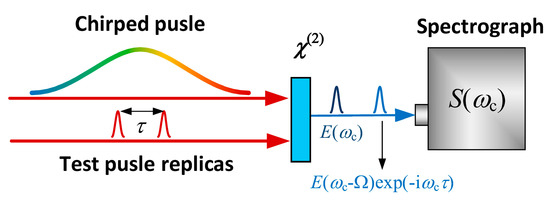
Figure 4.
Schematic of SPIDER. χ(2) is a nonlinear crystal. The fundamental (FH) pulse replicas are frequency-conversed in the nonlinear crystal with a shear Ω.
S(ω) = |E(ω)|2 + |E(ω − Ω)|2 + 2|E(ω)||E(ω − Ω)|cos[ωτ + φ(ω) − φ(ω − Ω)].
From S(ω), the differential phase θτ(ω) = φ(ω) − φ(ω − Ω) + ωτ can be easily extracted by Fourier domain filtering which was first suggested by Takeda et al. for applications in holography [57]:
where the integral region [τ − twin/2, τ + twin/2] is to filter the positive (or negative) alternating current (AC) term of the spectrum, twin is the width of the filter windows. The linear phase ωτ should be calibrated experimentally, to determine the differential phase θ(ω) = φ(ω) − φ(ω − Ω), by recording a reference interferogram without spectral shear additionally. The spectral phase φ(ω) can be obtained by concatenating θ(ω) [8]. If Ω is small sufficiently within that the spectral phase does not vary obviously, φ(ω) ≈ ∫θ(ω)dω/Ω. The algorithm of SPIDER is simple, robust, and direct compared to FROG, more easily supporting real-time display at a much higher frame rate.
There are two important development directions for SPIDER recently. One is to improve the capability for retrieving pulses those with complex temporal/spectral structure, e.g., few-cycle pulse, white-light supercontinuum. The other is to improve the usability or practicability of SPIDER, e.g., compactness, stability, robust, and cost.
In the original SPIDER, the pulse replicator based on MI brings unbalanced dispersions to the replicas then limits its application for ultra-broadband pulses. Zero-additional phase (ZAP) [58] SPIDER uses one FH test pulse and two chirped-pulse replicas, avoiding dispersive distortion by the unbalanced pulse replicator, and broaden the measuring spectral range of SPIDER to hundreds of nanometers.
Promoting the spectral resolution is much more challenging for shearing spectral interferometry. One of the causes is that spectral interferometry encodes the differential spectral phase into the interval of interferential fringes, so SPIDER should operate at a high spectral sampling rate typically 5~10 times of the Nyquist limit [59]. When we extract the phase from the interferogram, the spectral resolution is determined by the width of the temporal filtering window: Δωres~twin−1. Wavelet transform has been suggested [60,61] as a substitute of Fourier transform for phase retrieval, and proven to increase the filtering window thus the minimum of the required sampling rate by 20%. However, the wavelet transform has lower computational efficiency compared to the Fourier transform.
To relax the spectral resolution requirement of the spectrograph, a technique called spatially encoded arrangement for SPIDER (SEA-SPIDER) [59,62] is proposed, where two SF-beams cross into the spectrograph, and the interferential fringes are resolved in space-dimension. This method can operate for single-shot measurement. However, the measurement based on spatial interference is easily affected by the beam quality or imaging aberrations. Comparatively, two-dimensional spectral shearing interferometry (2DSI) [42,63,64], as shown in Figure 5, introduces a time-dimension instead of the space-dimension to resolve the interferential fringes, which can avoid the affection of the beam quality. Its “time interference”, causing by the minor delay between two pulse replicas, is similar to that in an interferential autocorrelator. The 2DSI-SPIDER need not determine the normal fringes-spacing for calibration. A disadvantage of 2DSI-SPIDER is that it cannot operate for single-shot measurement. Both SEA-and 2DSI-SPIDER are based on 2D measurement, needs inevitably more complex structures and expensive devices, e.g., imaging spectrograph for SEA-SPIDER, or motor-controlled element for 2DSI-SPIDER. Moreover, the recorded 2D data means a longer time required to process than the usual 1D data. Recently, we have successfully combined two-step phase-shifting (TSPS) into SPIDER [65], which can expend the filtering window to the positive (or negative) semi-axis in the Fourier domain by using 1D measurement. A quarter waveplate is inserted into one arm of the MI pulse replicator to control the zero-order additional phase at θ0 or θ0 + π, respectively, to generate two spectral interferograms with π phase-shifting. By combining these two interferograms, we can get the difference of two interferograms: ΔS(ω) = S(ω) − Sπ(ω) = 4|E(ω)||E(ω − Ω)|cos[ωτ + φ(ω) − φ(ω − Ω)], where the strong direct current (DC) term is canceled, helping to expend the width of the filtering window.
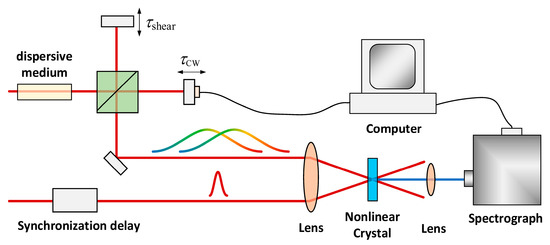
Figure 5.
Schematic of 2DSI optics. The SPIDER is based on a collinear ZAP geometry, in the vertical arm of MI, a minor delay is introduced to generate time interferential fringes.
There is another parameter, spectral shear Ω, that determines the resolution of the spectral phase. We obtain the spectral phase φ(ω) by concatenating the differential phase θ(ω) with an interval Ω. Smaller Ω means better spectral resolution. However, the choice of Ω is limited by the measured SNR. If Ω is chosen too small, the differential phase becomes unmeasurably small due to the detection noise [66]. Moreover, this noise is also accumulated in the course of phase concatenations. Small Ω leads to a large concatenation number, at the wavelengths far away from the central wavelength, the recovered phase noise becomes very large. For finite SNRs, SPIDERs usually work at relative shear Ω/ΔωBW = 4.6%~20% [7,8,60,62,63,66], where ΔωBW is the spectral bandwidth. D. Austin et al. [67] proposed a method called multiple-shearing spectral interferometry, where interferential data with different shears are combined to suppress the accumulating phase noise and improve the spectral resolution. This method is relatively complex, involving shear changes in the measurements. It also asks for a relatively high consistency of the multi-shear data. To improve the SNR of the SPIDER, we develop a complete-TSPS SPIDER (CTP-SPIDER) [68], where both the test spectrum and reference spectrum can introduce TSPS, as shown in Figure 6. Here, complete TSPS acts as a balanced detection that can not only remove the effect of the DC term of the interferogram but also reduce the measurement noises. Available shear can be down to 1.5% of the spectral width in this device.
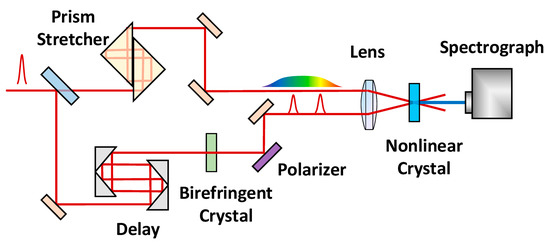
Figure 6.
Schematic of a compact SPIDER with a birefringent pulse replicator and a compact stretcher consisting of two oppositely placed rectangular prisms [68].
To improve the compactness and the robustness of the SPIDER, people propose some simplifications for SPIDER. The MI pulse replicator has two orthogonal light paths, which is take up more space. Moreover, it is very sensitive to the environment, easily causing jitters or shift between two pulse replicas, which is required to be controlled at a sub-fs level (or even 10 as for few-cycle pulses) [63]. A glass plate (or etalon) [66,69] causing multiple reflections is a substitute for MI. However, the output is a fade-out pulse train where the fade-in additional dispersions introducing to the sub-pulses. All-transmission pulse replicator [70,71] based on birefringence is a better substitute, where the optical axis of the birefringence crystal is set at 45° relative to the polarization of the input light. The o-ray and e-ray pulses separate with a delay for their different group-velocities. In this replicator, the dispersion difference between the o-ray and e-ray inducing an additional dispersion, which is much lower than that by etalon or beamsplitter of MI, thus can be applied to characterize the few-cycle pulses [71]. Reference [71] also shows that such common-path, all-transmission pulse replicator can improve the SNR by a factor of 3.7. Table 2 shows a comparison of some SPIDER geometries on the operating mode, data-dimension, spectral resolution, shear, phase error, et al.
An approach based on the asymmetric phase-matching function [8] to generate spectral shear without a pulse stretcher was proposed [70,72,73]. The pulse stretcher can be removed in this configuration. The highly asymmetric phase-matching function is due to group-velocity matching between FH o-ray with SF and group-velocity mismatching between FH e-ray with SF for a type-II χ(2)-medium. In such a medium, the acceptance bandwidth can be designed very large at the o-axis whereas very narrow at the e-axis. Thus, the e-polarized FH acts as quasi-monochromatic light to carry the o-polarized FH to high frequency without altering the spectral phase. The phase-matching function is angularly dependent, two beams at slightly different propagation angles will therefore generate spectrally sheared upconverted replicas.
Table 2.
Comparison of some SPIDER geometries.
Table 2.
Comparison of some SPIDER geometries.
| SPIDER Geometry | Traditional | TSPS/CTP [65,68] | CP [71] | 2DSI [13] |
|---|---|---|---|---|
| Operating Mode | Single-shot | Single-shot | Single-shot | Multi-shot Scanning |
| Acquire data | 1D | 1D × 21 | 1D/1D × 2 | 2D |
| Spectral resolution 2 | 5~10 Δωres | ~2 Δωres | ~2 Δωres | ~ Δωres |
| Shear 3 | 0.1~0.2 ΔωBW | ~0.015 ΔωBW | ~0.03 ΔωBW | ~0.05 ΔωBW |
| Phase error (3dB bandwidth) | ~44 mrad [74] | 74.2 mrad (TSPS) 19.3 mrad (CTP) | 2.6 mrad | Unspecified |
1 Two 1D-interferograms. 2 Δωres is the resolution of the used spectrograph. 3 ΔωBW is the spectral width of the pulses.
In 2010, a new method called Self-Referenced Spectral Interferometry (SRSI) [13] for femtosecond pulses characterization was introduced. Different from the shearing interferometry, SRSI is a linear method like traditional interferometry with no need for neither shear nor SF generation. In SRSI, the reference pulse is generated from the unknown test pulse based on Crossed-Polarized Wave generation (XPW), and the reference field can be written as Eref(t)~|Etest(t)|2Etest(t), where Etest(t) is the test field. Here, the XPW acts as a time filter [75], and flatten the spectral phase. The phase extracted directly from the interferogram can get a rough estimation of the phase. To obtain an accurate result, several iterations of algorithms are needed. The use of third-order nonlinear optical processes, need not consider the phase-matching compared to SPIDER using χ(2)-nonlinear, however, has a higher energy requirement. Except XPW [13,31], other χ(3)-nonlinear generation can also be considered in SRSI, such as SD [76,77] or TG [78,79].
6. Conclusions and Prospect
In the paper, we classify the self-reference measurements for ultrashort pulse into three categories: Correlation, Spectrogram, and Spectral Interferometry. Correlation is a time-domain technique. It obtains rough time information of the pulse by delaying the interactional pulses in a nonlinear crystal. For its simple geometry and measurement, correlation has very high measuring SNR, which makes it irreplaceable in the measurement of contrast for high power lasers. The Spectrogram technique is a 2D ω-ξ-combined measurement, ξ can be the time delay (FROG) or other scanning parameters (e.g., dispersion in d-scan, phase of spectral modulation function in MIIPS). Benefiting by their time-frequency over-determine, FROG has its superiority in drawing complex pulses, meanwhile, the pulse retrieval needs a time-consuming iteration algorithm. Spectral Interferometry (including SPIDER and SRSI) is based on spectral measurement by coding the spectral phase into the interferential fringes. Spectral Interferometry has a direct, robust retrieval algorithm supporting real-time display at a very high frame rate. Interferometry, especially shearing interferometry, has a high requirement for the resolution of the spectrograph when applied to complex pulses.
In the future, ultrashort pulse lasers will have higher peak power, more complex pulses, and/or more diverse wavelengths, which bring higher and new requirements for their measurements. In high power laser region, 10 PW level lasers with a focused intensity of ~1022 W/cm2 have been realized in many countries or regions, and to build 100-PW-level lasers is on the agenda. This demands the Correlator can work with ultrahigh SNR (>1012), single-shot, space-resolved technique (a recent study [80] shows that spatiotemporal noise also impacts the far-field contrast). Nowadays, with the developments of the ultrafast laser technology and the optical manipulations, the forms of ultrashort light fields become more and more abundant. In some scenes, such as few-/single-cycle pulses generation, white-light supercontinuum induced by Kerr effects, spectral coherent synthesis, and spectral modulation for quantum coherent control, the pulse structures have comparative complex in the temporal domain, which requires the measurements to have a high temporal resolution. While in some other scenes, the identity of the pulse characteristics in space is broken, where spatiotemporal measurement capability becomes important. For example, in optical parametric amplification (OPA) or optical rectification for THz generation, the pulse-front title is induced to realize velocity-matching to improve the energy conversion efficiency or the bandwidth; for vortex beams or other optical fields by spatial manipulation, the pulse characteristics depend on spatial distribution; for few-cycle pulses, the spatiotemporal coupling effect becomes sensitive for its very broad bandwidth. In the past, measurement techniques are mostly designed for ultrafast lasers in the near-infrared (IR). Nowadays, more requirements in other wavebands are put forward. Mid-IR lasers [81,82] are found to have their unique advantages in some fields, such as particle acceleration or high-order harmonic generation. In the mid-IR region, due to the lack of elements, nonlinear crystal, and difficulty for coating, the development of measurement techniques is far behind that in the near-IR. In the ultraviolet (UV) region, the ultrashort pulse characterization meets the challenges by nonlinear optics. Common nonlinear crystals, e.g., potassium dihydrogen phosphate (KDP), beta-barium borate (BBO), or lithium triborate (LBO), the minimal FH wavelengths for frequency-doubling are no shorter than 410 nm, which limited the application of frequency up-conversion in the ultrashort pulse measurements. In visible or UV regions, the dispersion as well as the group-velocity mismatching inside the crystals is usually much larger than that near-IR, which limits the bandwidth of frequency conversion. In recent years, fiber ultrafast lasers have greatly progressed, for the high stability and average power, and have been largely applied in many fields, especially in the manufacturing industry. Fiber ultrafast lasers have longer pulse widths, up to ~100fs or longer, compared to solid ultrafast lasers, which means it has narrower bandwidths. To completely characterizing such pulses, the resolution of the spectrograph becomes critical. FROG, as a time-frequency combination measurement has its disadvantage in the real-time display for the time-consuming algorithm, which can be alleviated by improving the computer performance. For SPIDER, SEA/TSPS can improve the capability in the measurement of long pulses or the pulses with complex structures without degrading the real-time performance. Considering the cost, TSPS-SPIDER may be a better candidate.
Author Contributions
Conceptualization, writing, drawing, funding acquisition, Y.C.; writing, editing, Z.C.; project administration, X.Z.; editing, H.S.; review, funding acquisition, X.L.; review, Q.S.; project administration, Y.A.; review, funding acquisition, S.X.; funding acquisition, J.L. All authors have read and agreed to the published version of the manuscript.
Funding
This work was supported by Natural Science Foundation of China (61775142, 61827815, 61705132, 62075138), Shenzhen Fundamental Research Project (JCYJ20190808164007485, JCYJ20190808121817100, JCYJ20190808115601653), and Postgraduate innovation development fund project of Shenzhen University (315-0000470506).
Conflicts of Interest
The authors declare no conflict of interest.
References
- Li, W.Q.; Gan, Z.B.; Yu, L.H.; Wang, C.; Liu, Y.Q.; Guo, Z.; Xu, L.; Xu, M.; Hang, Y.; Xu, Y.; et al. 339 j high-energy ti:Sapphire chirped-pulse amplifier for 10 pw laser facility. Opt. Lett. 2018, 43, 5681–5684. [Google Scholar] [CrossRef] [PubMed]
- Guo, Z.; Yu, L.H.; Wang, J.Y.; Wang, C.; Liu, Y.Q.; Gan, Z.B.; Li, W.Q.; Leng, Y.X.; Liang, X.Y.; Li, R.X. Improvement of the focusing ability by double deformable mirrors for 10-pw-level ti: Sapphire chirped pulse amplification laser system. Opt. Express 2018, 26, 26776–26786. [Google Scholar] [CrossRef]
- Yoon, J.W.; Jeon, C.; Shin, J.; Lee, S.K.; Lee, H.W.; Choi, I.W.; Kim, H.T.; Sung, J.H.; Nam, C.H. Achieving the laser intensity of 5.5×10^22 w/cm2 with a wavefront-corrected multi-pw laser. Opt. Express 2019, 27, 20412–20420. [Google Scholar] [CrossRef] [PubMed]
- Wirth, A.; Hassan, M.T.; Grguras, I.; Gagnon, J.; Moulet, A.; Luu, T.T.; Pabst, S.; Santra, R.; Alahmed, Z.A.; Azzeer, A.M.; et al. Synthesized light transients. Science 2011, 334, 195–200. [Google Scholar] [CrossRef] [PubMed]
- Bradley, D.J.; Liddy, B.; Sleat, W.E. Direct linear measurement of ultrashort light pulses with a picosecond streak camera. Opt. Commun. 1971, 2, 391–395. [Google Scholar] [CrossRef]
- Etchepare, J.; Grillon, G.; Orszag, A. Third order autocorrelation study of amplified subpicosecond laser pulses. IEEE J. Quantum Electron. 1983, 19, 775–778. [Google Scholar] [CrossRef]
- Iaconis, C.; Walmsley, I.A. Spectral phase interferometry for direct electric-field reconstruction of ultrashort optical pulses. Opt. Lett. 1998, 23, 792–794. [Google Scholar] [CrossRef]
- Iaconis, C.; Walmsley, I.A. Self-referencing spectral interferometry for measuring ultrashort optical pulses. IEEE J. Quantum Electron. 1999, 35, 501–509. [Google Scholar] [CrossRef]
- O’Shea, P.; Kimmel, M.; Gu, X.; Trebino, R. Highly simplified device for ultrashort-pulse measurement. Opt. Lett. 2001, 26, 932–934. [Google Scholar] [CrossRef]
- Janszky, J.; Corradi, G. Full intensity profile analysis of ultrashort laser pulses using four-wave mixing or third harmonic generation. Opt. Commun. 1986, 60, 251–256. [Google Scholar] [CrossRef]
- Kane, D.J.; Trebino, R. Single-shot measurement of the intensity and phase of an arbitrary ultrashort pulse by using frequency-resolved optical gating. Opt. Lett. 1993, 18, 823–825. [Google Scholar] [CrossRef] [PubMed]
- Trebino, R.; DeLong, K.W.; Fittinghoff, D.N.; Sweetser, J.N.; Krumbugel, M.A.; Richman, B.A.; Kane, D.J. Measuring ultrashort laser pulses in the time-frequency domain using frequency-resolved optical gating. Rev. Sci. Instrum. 1997, 68, 3277–3295. [Google Scholar] [CrossRef]
- Oksenhendler, T.; Coudreau, S.; Forget, N.; Crozatier, V.; Grabielle, S.; Herzog, R.; Gobert, O.; Kaplan, D. Self-referenced spectral interferometry. Appl. Phys. B 2010, 99, 7–12. [Google Scholar] [CrossRef]
- Hu, Y.; Tehranchi, A.; Wabnitz, S.; Kashyap, R.; Chen, Z.; Morandotti, R. Improved intrapulse Raman scattering control via asymmetric airy pulses. Phys. Rev. Lett. 2015, 114, 073901. [Google Scholar] [CrossRef] [PubMed]
- Husakou, A.V.; Herrmann, J. Supercontinuum generation of higher-order solitons by fission in photonic crystal fibers. Phys. Rev. Lett. 2001, 87, 203901. [Google Scholar] [CrossRef]
- Trebino, R. Frequency-Resolved Optical Gating: The Measurement of Ultrashort Laser Pulses; Kluwer Academic Publishers: Boston, MA, USA, 2002; pp. 16–17. [Google Scholar]
- Oriana, A.; Réhault, J.; Preda, F.; Polli, D.; Cerullo, G. Scanning Fourier transform spectrometer in the visible range based on birefringent wedges. J. Opt. Soc. Am. A 2016, 33, 1415–1420. [Google Scholar] [CrossRef]
- Adler, F.; Maslowski, P.; Foltynowicz, A.; Cossel, K.C.; Briles, T.C.; Hartl, I.; Ye, J. Mid-infrared fourier transform spectroscopy with a broadband frequency comb. Opt. Express 2010, 18, 21861–21872. [Google Scholar] [CrossRef]
- Diels, J.-C.M.; Fontaine, J.J.; McMichael, I.C.; Simoni, F. Control and measurement of ultrashort pulse shapes (in amplitude and phase) with femtosecond accuracy. Appl. Opt. 1985, 24, 1270–1282. [Google Scholar] [CrossRef]
- Diels, J.-C.; Van Stryland, E.; Benedict, G. Generation and measurement of 200 femtosecond optical pulses. J. Opt. Soc. Am. 1978, 68, 666. [Google Scholar] [CrossRef]
- Diels, J.-C.; Rudolph, W. Ultrashort Laser Pulse Phenomena, 2nd ed.; Academic Press: San Diego, CA, USA, 1996. [Google Scholar]
- Available online: https://www.ape-berlin.de/en/autocorrelator/ (accessed on 22 October 2020).
- Available online: http://www.lightcon.com/Products/autocorrelators.html (accessed on 22 October 2020).
- Available online: https://www.edmundoptics.com/f/edmund-optics-ultrafast-autocorrelator-by-ape/39533/ (accessed on 22 October 2020).
- Wang, Y.; Ma, J.; Wang, J.; Yuan, P.; Xie, G.; Ge, X.; Liu, F.; Yuan, X.; Zhu, H.; Qian, L. Single-shot measurement of >1010 pulse contrast for ultra-high peak-power lasers. Sci. Rep. 2014, 4, 3818. [Google Scholar] [CrossRef]
- Luan, S.; Hutchinson, M.H.R.; Smith, R.A.; Zhou, F. High dynamic range third-order correlation measurement of picosecond laser pulse shapes. Meas. Sci. Technol. 1993, 4, 1426–1429. [Google Scholar] [CrossRef]
- Divall, E.J.; Ross, I.N. High dynamic range contrast measurements by use of an optical parametric amplifier correlator. Opt. Lett. 2004, 29, 2273–2275. [Google Scholar] [CrossRef] [PubMed]
- Dorrer, C.; Bromage, J.; Zuegel, J.D. High-dynamic-range single-shot cross-correlator based on an optical pulse replicator. Opt. Express 2008, 16, 13534–13544. [Google Scholar] [CrossRef] [PubMed]
- Shah, R.C.; Johnson, R.P.; Shimada, T.; Hegelich, B.M. Large temporal window contrast measurement using optical parametric amplification and low-sensitivity detectors. Eur. Phys. J. D 2009, 55, 305–309. [Google Scholar] [CrossRef]
- Wang, Y.Z.; Yuan, P.; Ma, J.G.; Qian, L.J. Scattering noise and measurement artifacts in a single-shot cross-correlator and their suppression. Appl. Phys. B 2013, 111, 501–508. [Google Scholar] [CrossRef]
- Wang, P.; Shen, X.; Liu, J.; Li, R. Single-shot fourth-order autocorrelator. Adv. Photonics 2019, 1, 056001. [Google Scholar] [CrossRef]
- Cohen, L. Time-Frequency Analysis: Theory and Applications; Prentice Hall: Englewood Cliffs, NJ, USA, 1995. [Google Scholar]
- Stark, H. Image Recovery: Theory and Application; Academic Press: Orlando, FL, USA, 1987. [Google Scholar]
- Clement, T.S.; Taylor, A.J.; Kane, D.J. Single-shot measurement of the amplitude and phase of ultrashort laser pulses in the violet. Opt. Lett. 1995, 20, 70–72. [Google Scholar] [CrossRef]
- Sweetser, J.N.; Fittinghoff, D.N.; Trebino, R. Transient-grating frequency-resolved optical gating. Opt. Lett. 1997, 22, 519–521. [Google Scholar] [CrossRef]
- Trebino, R. Frequency-Resolved Optical Gating: The Measurement of Ultrashort Laser Pulses; Kluwer Academic Publishers: Boston, MA, USA, 2000; pp. 117–137. [Google Scholar]
- Available online: http://www.swampoptics.com/index.html (accessed on 22 October 2020).
- Stibenz, G.; Steinmeyer, G. Interferometric frequency-resolved optical gating. Opt. Express 2005, 13, 2617–2626. [Google Scholar] [CrossRef]
- Linden, S.; Kuhl, J.; Giessen, H. Amplitude and phase characterization of weak blue ultrashort pulses by downconversion. Opt. Lett. 1999, 24, 569–571. [Google Scholar] [CrossRef]
- Available online: http://www.swampoptics.com/ (accessed on 22 October 2020).
- Rhodes, M.; Steinmeyer, G.; Ratner, J.; Trebino, R. Pulse-shape instabilities and their measurement. Laser Photonics Rev. 2013, 7, 557–565. [Google Scholar] [CrossRef]
- Rhodes, M.; Mukhopadhyay, M.; Birge, J.; Trebino, R. Coherent artifact study of two-dimensional spectral shearing interferometry. J. Opt. Soc. Am. B 2015, 32, 1881–1888. [Google Scholar] [CrossRef]
- Lozovoy, V.V.; Pastirk, I.; Dantus, M. Multiphoton intrapulse interference. Iv. Ultrashort laser pulse spectral phase characterization and compensation. Opt. Lett. 2004, 29, 775–777. [Google Scholar] [CrossRef]
- Lozovoy, V.V.; Xu, B.; Coello, Y.; Dantus, M. Direct measurement of spectral phase for ultrashort laser pulses. Opt. Express 2008, 16, 592–597. [Google Scholar] [CrossRef]
- Xu, B.W.; Gunn, J.M.; Dela Cruz, J.M.; Lozovoy, V.V.; Dantus, M. Quantitative investigation of the multiphoton intrapulse interference phase scan method for simultaneous phase measurement and compensation of femtosecond laser pulses. J. Opt. Soc. Am. B 2006, 23, 750–759. [Google Scholar] [CrossRef]
- Comin, A.; Ciesielski, R.; Piredda, G.; Donkers, K.; Hartschuh, A. Compression of ultrashort laser pulses via gated multiphoton intrapulse interference phase scans. J. Opt. Soc. Am. B 2014, 31, 1118–1125. [Google Scholar] [CrossRef]
- Miranda, M.; Fordell, T.; Arnold, C.; L’Huillier, A.; Crespo, H. Simultaneous compression and characterization of ultrashort laser pulses using chirped mirrors and glass wedges. Opt. Express 2012, 20, 688–697. [Google Scholar] [CrossRef]
- Miranda, M.; Arnold, C.L.; Fordell, T.; Silva, F.; Alonso, B.; Weigand, R.; L’Huillier, A.; Crespo, H. Characterization of broadband few-cycle laser pulses with the d-scan technique. Opt. Express 2012, 20, 18732–18743. [Google Scholar] [CrossRef]
- Canhota, M.; Silva, F.A.D.; Weigand, R.; Crespo, H. Inline self-diffraction dispersion-scan of over octave-spanning pulses in the single-cycle regime. Opt. Lett. 2017, 42, 3048–3051. [Google Scholar] [CrossRef] [PubMed]
- Tajalli, A.; Kalousdian, T.K.; Kretschmar, M.; Kleinert, S.; Morgner, U.; Nagy, T. Full characterization of 8 fs deep uv pulses via a dispersion scan. Opt. Lett. 2019, 44, 2498–2501. [Google Scholar] [CrossRef]
- Tajalli, A.; Ouille, M.; Vernier, A.; Bohle, F.; Escoto, E.; Kleinert, S.; Romero, R.; Csontos, J.; Morgner, U.; Steinmeyer, G. Propagation effects in the characterization of 1.5-cycle pulses by xpw dispersion scan. IEEE J. Sel. Top. Quant. 2019, 25, 1–7. [Google Scholar] [CrossRef]
- Spangenberg, D.; Rohwer, E.G.; Brugmann, M.; Feurer, T. Ptychographic ultrafast pulse reconstruction. Opt. Lett. 2015, 40, 1002–1005. [Google Scholar] [CrossRef] [PubMed]
- Witting, T.; Greening, D.; Walke, D.; Matia-Hernando, P.; Barillot, T.; Marangos, J.P.; Tisch, J.W.G. Time-domain ptychography of over-octave-spanning laser pulses in the single-cycle regime. Opt. Lett. 2016, 41, 4218. [Google Scholar] [CrossRef] [PubMed]
- Loriot, V.; Gitzinger, G.; Forget, N. Self-referenced characterization of femtosecond laser pulses by chirp scan. Opt. Express 2013, 21, 24879. [Google Scholar] [CrossRef] [PubMed]
- Meshulach, D.; Silberberg, Y. Coherent quantum control of two-photon transitions by a femtosecond laser pulse. Nature 1998, 396, 239–242. [Google Scholar] [CrossRef]
- Geib, N.C.; Zilk, M.; Pertsch, T.; Eilenberger, F. Common pulse retrieval algorithm: A fast and universal method to retrieve ultrashort pulses. Optica 2019, 6, 495–505. [Google Scholar] [CrossRef]
- Takeda, M.; Ina, H.; Kobayashi, S. Fourier-transform method of fringe-pattern analysis for computer-based topography and interferometry. J. Opt. Soc. Am. 1982, 72, 156–160. [Google Scholar] [CrossRef]
- Baum, P.; Lochbrunner, S.; Riedle, E. Zero-additional-phase spider: Full characterization of visible and sub-20-fs ultraviolet pulses. Opt. Lett. 2004, 29, 210–212. [Google Scholar] [CrossRef]
- Kosik, E.M.; Radunsky, A.S.; Walmsley, I.A.; Dorrer, C. Interferometric technique for measuring broadband ultrashort pulses at the sampling limit. Opt. Lett. 2005, 30, 326–328. [Google Scholar] [CrossRef]
- Bethge, J.; Grebing, C.; Steinmeyer, G. A fast gabor wavelet transform for high-precision phase retrieval in spectral interferometry. Opt. Express 2007, 15, 14313–14321. [Google Scholar] [CrossRef]
- Deng, Y.; Wang, C.; Chai, L.; Zhang, Z. Determination of gabor wavelet shaping factor for accurate phase retrieval with wavelet-transform. Appl. Phys. B 2005, 81, 1107–1111. [Google Scholar] [CrossRef]
- Wyatt, A.S.; Walmsley, I.A.; Stibenz, G.; Steinmeyer, G. Sub-10 fs pulse characterization using spatially encoded arrangement for spectral phase interferometry for direct electric field reconstruction. Opt. Lett. 2006, 31, 1914–1916. [Google Scholar] [CrossRef] [PubMed]
- Birge, J.R.; Ell, R.; Kärtner, F.X. Two-dimensional spectral shearing interferometry for few-cycle pulse characterization. Opt. Lett. 2006, 31, 2063–2065. [Google Scholar] [CrossRef] [PubMed]
- Birge, J.R.; Kärtner, F.X. Analysis and mitigation of systematic errors in spectral shearing interferometry of pulses approaching the single-cycle limit [invited]. J. Opt. Soc. Am. B 2008, 25, A111–A119. [Google Scholar] [CrossRef]
- Zheng, S.; Cai, Y.; Pan, X.; Zeng, X.; Li, J.; Li, Y.; Zhu, T.; Lin, Q.; Xu, S. Two-step phase-shifting SPIDER. Sci. Rep. 2016, 6, 33837. [Google Scholar] [CrossRef]
- Gero Stibenz, G.S. Optimizing spectral phase interferometry for direct electric-field reconstruction. Rev. Sci. Instrum. 2006, 77, 073105. [Google Scholar] [CrossRef]
- Austin, D.R.; Witting, T.; Walmsley, I.A. High precision self-referenced phase retrieval of complex pulses with multiple-shearing spectral interferometry. J. Opt. Soc. Am. B 2009, 26, 1818–1830. [Google Scholar] [CrossRef]
- Cai, Y.; Chen, Z.K.; Zheng, S.Q.; Lin, Q.G.; Zeng, X.K.; Li, Y.; Li, J.Z.; Xu, S.X. Accurate reconstruction of electric field of ultrashort laser pulse with complete two-step phase-shifting. High. Power Laser Sci. 2019, 7, e13. [Google Scholar] [CrossRef]
- Anderson, M.E.; Witting, T.; Walmsley, I.A. Gold-spider: Spectral phase interferometry for direct electric field reconstruction utilizing sum-frequency generation from a gold surface. J. Opt. Soc. Am. B 2008, 25, A13–A16. [Google Scholar] [CrossRef]
- Gorza, S.P.; Radunsky, A.S.; Wasylczyk, P.; Walmsley, I.A. Tailoring the phase-matching function for ultrashort pulse characterization by spectral shearing interferometry. J. Opt. Soc. Am. B 2007, 24, 2064–2074. [Google Scholar] [CrossRef]
- Cai, Y.; Chen, Z.; Zheng, S.; Shangguan, H.; Zeng, X.; Lu, X.; Wang, H.; Xu, S. A compact, highly stable spectral shearing interferometer to accurately reconstruct ultrafast laser fields. Opt. Lasers Eng. 2020, 130, 106081. [Google Scholar] [CrossRef]
- Radunsky, A.S.; Kosik Williams, E.M.; Walmsley, I.A.; Wasylczyk, P.; Wasilewski, W.; U’Ren, A.B.; Anderson, M.E. Simplified spectral phase interferometry for direct electric-field reconstruction by using a thick nonlinear crystal. Opt. Lett. 2006, 31, 1008–1010. [Google Scholar] [CrossRef] [PubMed]
- Radunsky, A.S.; Walmsley, I.A.; Gorza, S.-P.; Wasylczyk, P. Compact spectral shearing interferometer for ultrashort pulse characterization. Opt. Lett. 2007, 32, 181–183. [Google Scholar] [CrossRef]
- Gallmann, L.; Sutter, D.H.; Matuschek, N.; Steinmeyer, G.; Keller, U. Techniques for the characterization of sub-10-fs optical pulses: A comparison. Appl. Phys. B 2000, 70, S67–S75. [Google Scholar] [CrossRef]
- Oksenhendler, T. Self-referenced spectral interferometry theory. arXiv 2012, arXiv:1204.4949. [Google Scholar]
- Liu, J.; Jiang, Y.; Kobayashi, T.; Li, R.; Xu, Z. Self-referenced spectral interferometry based on self-diffraction effect. J. Opt. Soc. Am. B 2012, 29, 29–34. [Google Scholar] [CrossRef]
- Birkholz, S.; Steinmeyer, G.; Koke, S.; Gerth, D.; Bürger, S.; Hofmann, B. Phase retrieval via regularization in self-diffraction-based spectral interferometry. J. Opt. Soc. Am. B 2015, 32, 983–992. [Google Scholar] [CrossRef]
- Liu, J.; Li, F.J.; Jiang, Y.L.; Li, C.; Leng, Y.X.; Kobayashi, T.; Li, R.X.; Xu, Z.Z. Transient-grating self-referenced spectral interferometry for infrared femtosecond pulse characterization. Opt. Lett. 2012, 37, 4829–4831. [Google Scholar] [CrossRef]
- Shen, X.; Wang, P.; Liu, J.; Li, R.X. Compact transient-grating self-referenced spectral interferometry for sub-nanojoule femtosecond pulse characterization. Appl. Opt. 2017, 56, 582–586. [Google Scholar] [CrossRef]
- Ma, J.; Yuan, P.; Wang, J.; Wang, Y.; Xie, G.; Zhu, H.; Qian, L. Spatiotemporal noise characterization for chirped-pulse amplification systems. Nat. Commun. 2015, 6, 6192. [Google Scholar] [CrossRef]
- Pires, H.; Baudisch, M.; Sanchez, D.; Hemmer, M.; Biegert, J. Ultrashort pulse generation in the mid-ir. Prog. Quantum Electron. 2015, 43, 1–30. [Google Scholar] [CrossRef]
- Shumakova, V.; Malevich, P.; Ališauskas, S.; Voronin, A.; Zheltikov, A.M.; Faccio, D.; Kartashov, D.; Baltuška, A.; Pugžlys, A. Multi-millijoule few-cycle mid-infrared pulses through nonlinear self-compression in bulk. Nat. Commun. 2016, 7, 12877. [Google Scholar] [CrossRef] [PubMed]


Publisher’s Note: MDPI stays neutral with regard to jurisdictional claims in published maps and institutional affiliations. |
© 2020 by the authors. Licensee MDPI, Basel, Switzerland. This article is an open access article distributed under the terms and conditions of the Creative Commons Attribution (CC BY) license (http://creativecommons.org/licenses/by/4.0/).