Comparative Study on Exponentially Weighted Moving Average Approaches for the Self-Starting Forecasting


Abstract
1. Introduction
2. Background
2.1. Exponentially Weighted Moving Average Model
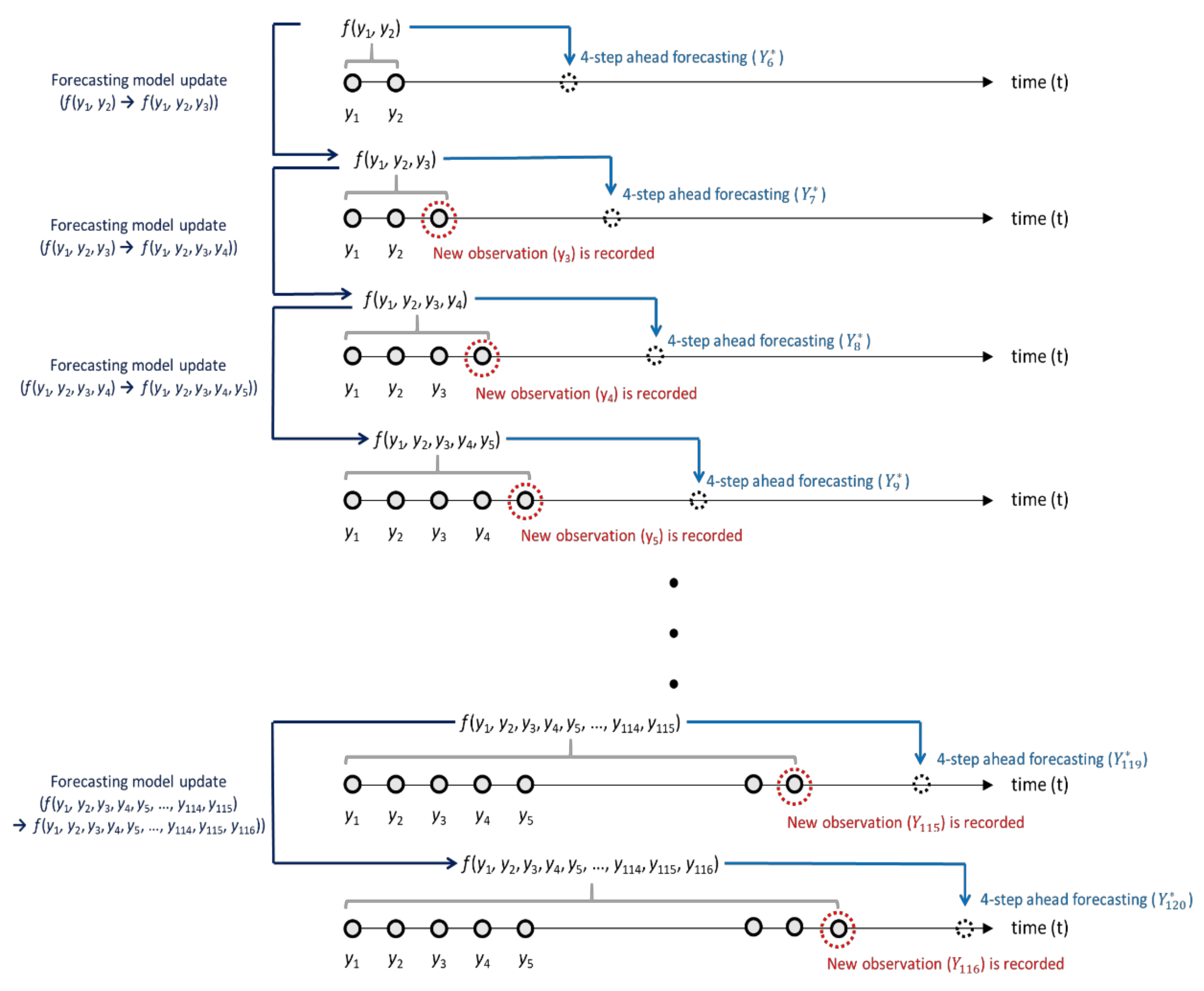
2.2. Self-Starting Forecasting Process with EWMA Model
3. Simulation Study
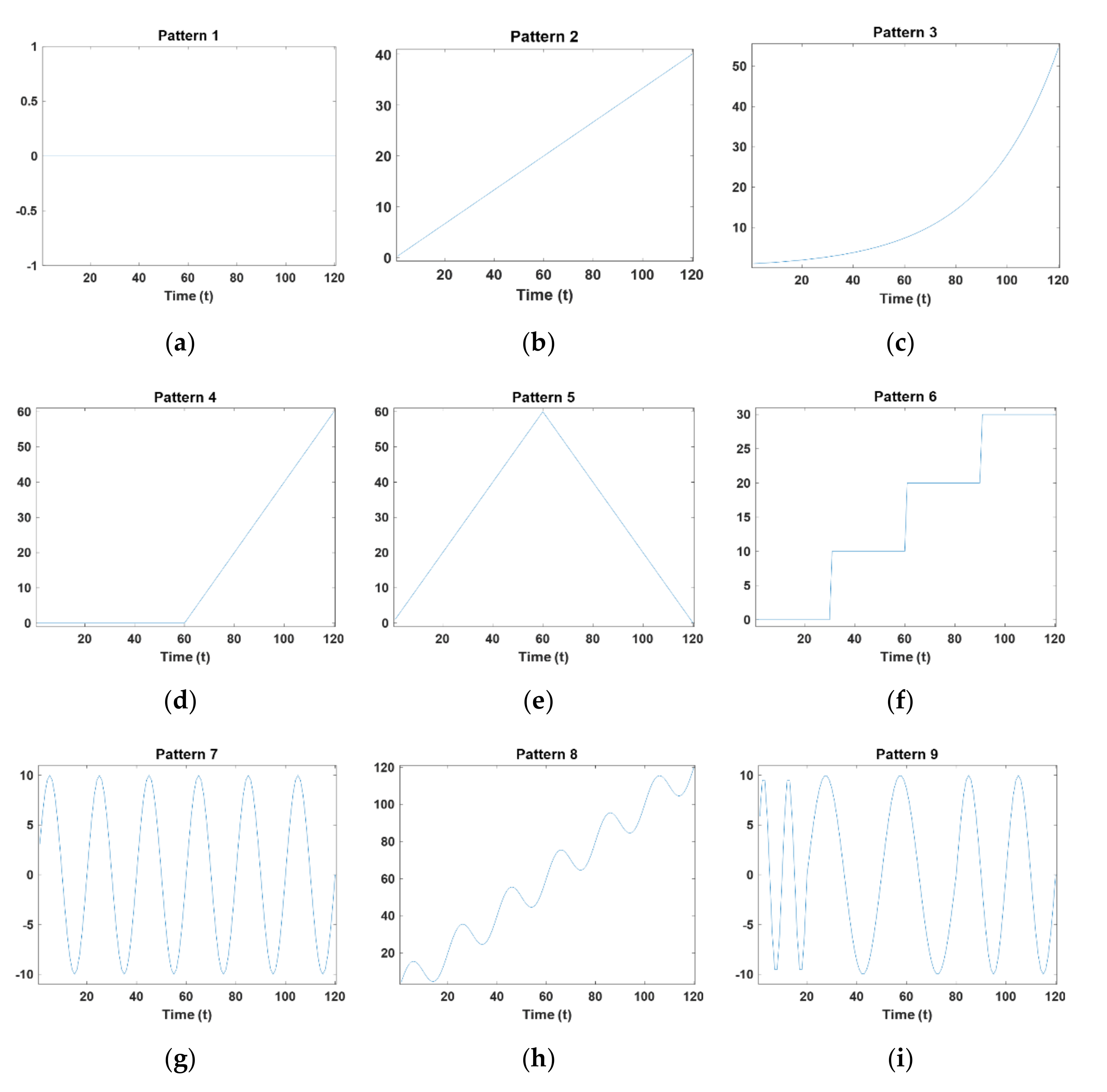
3.1. Simulation Setup
- Pattern 1: ;
- Pattern 2: ;
- Pattern 3: ;
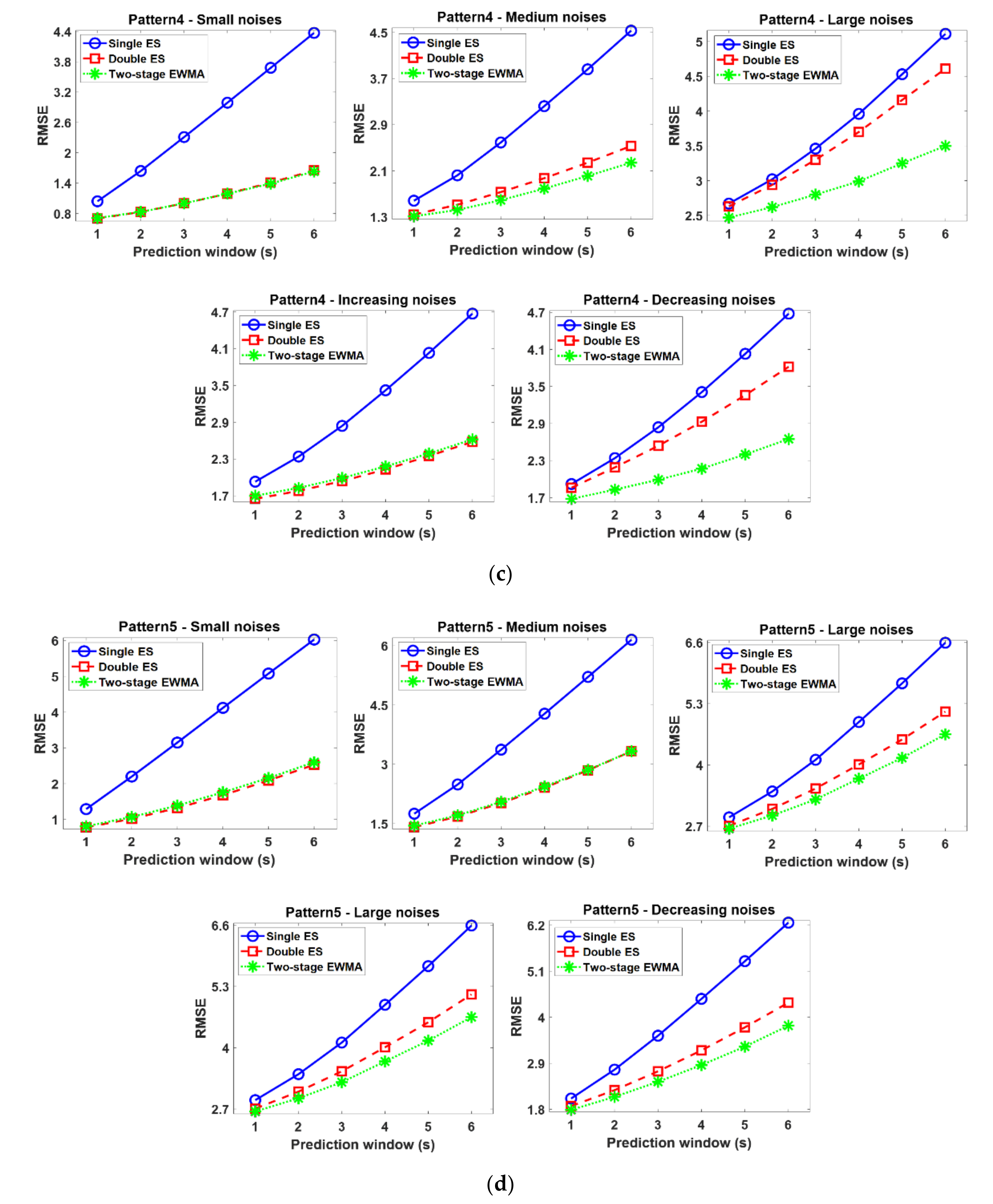
- Pattern 4:;
- Pattern 5: ;
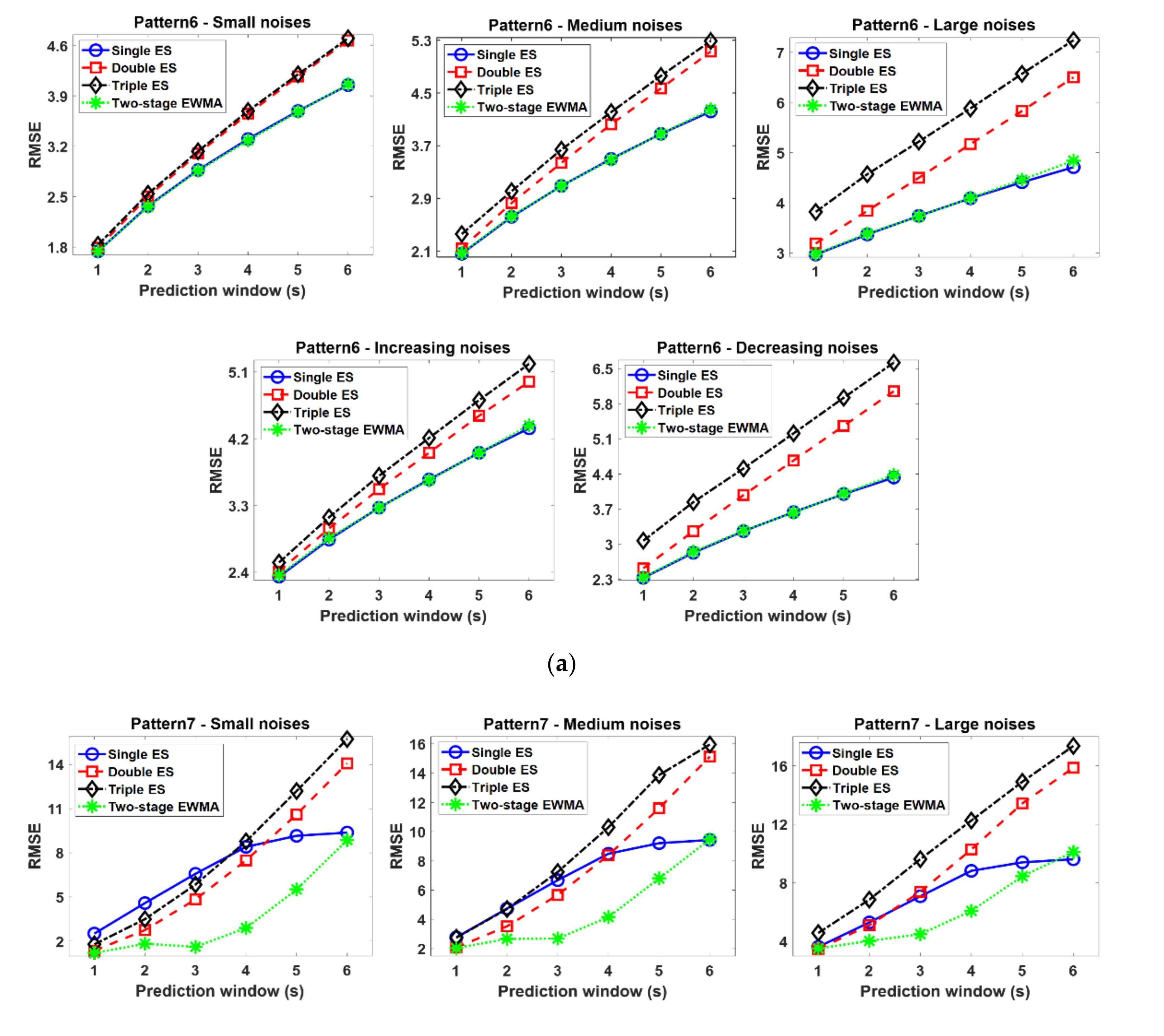
- Pattern 6: ;
- Pattern 7: ;
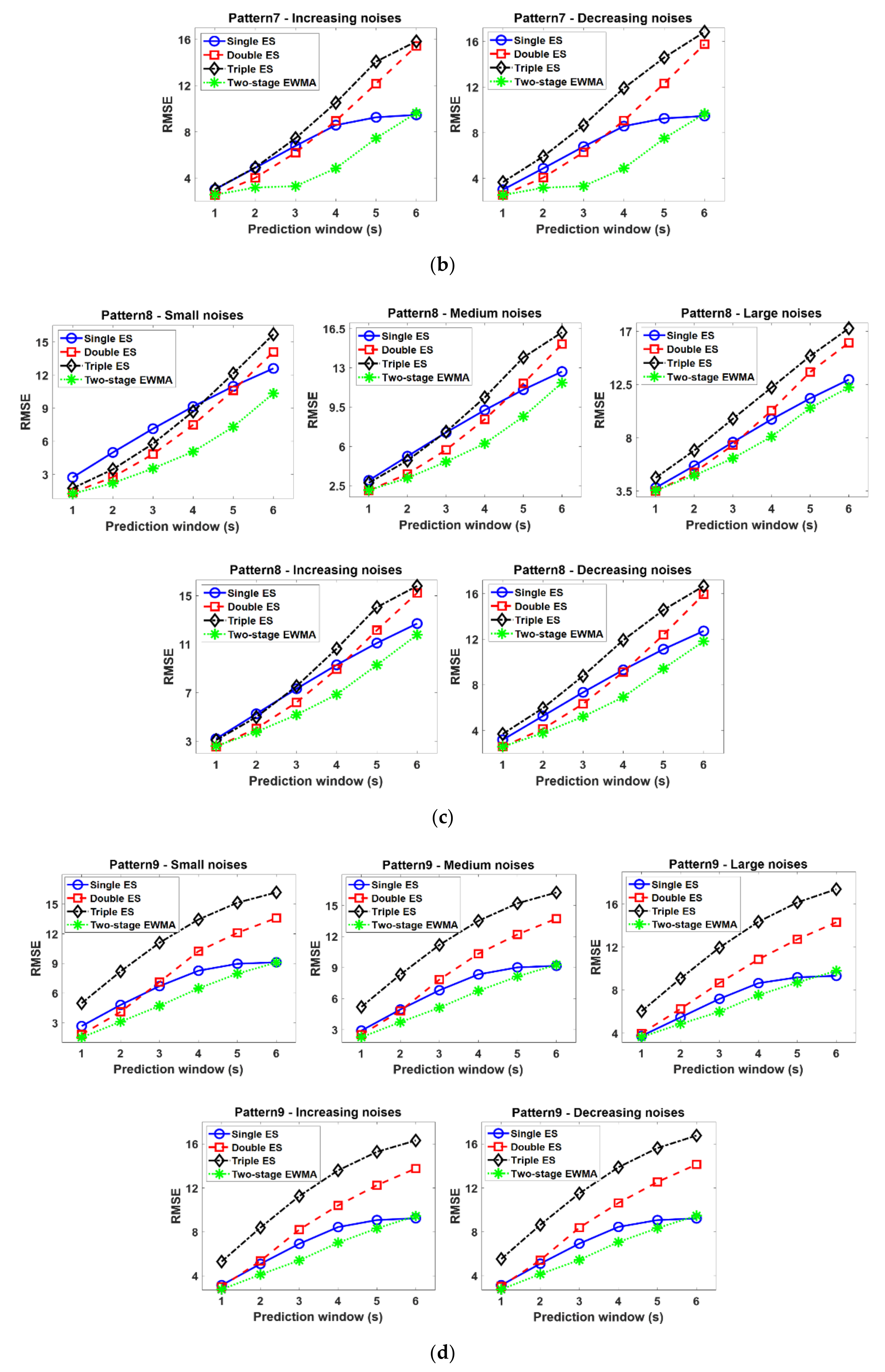
- Pattern 8: ;
- Pattern 9: .
- Small noise (homoscedastic): ;
- Medium noise (homoscedastic): ;
- Large noise (homoscedastic):
- Increasing noise (heteroscedastic): ;
- Deceasing noise (heteroscedastic): .
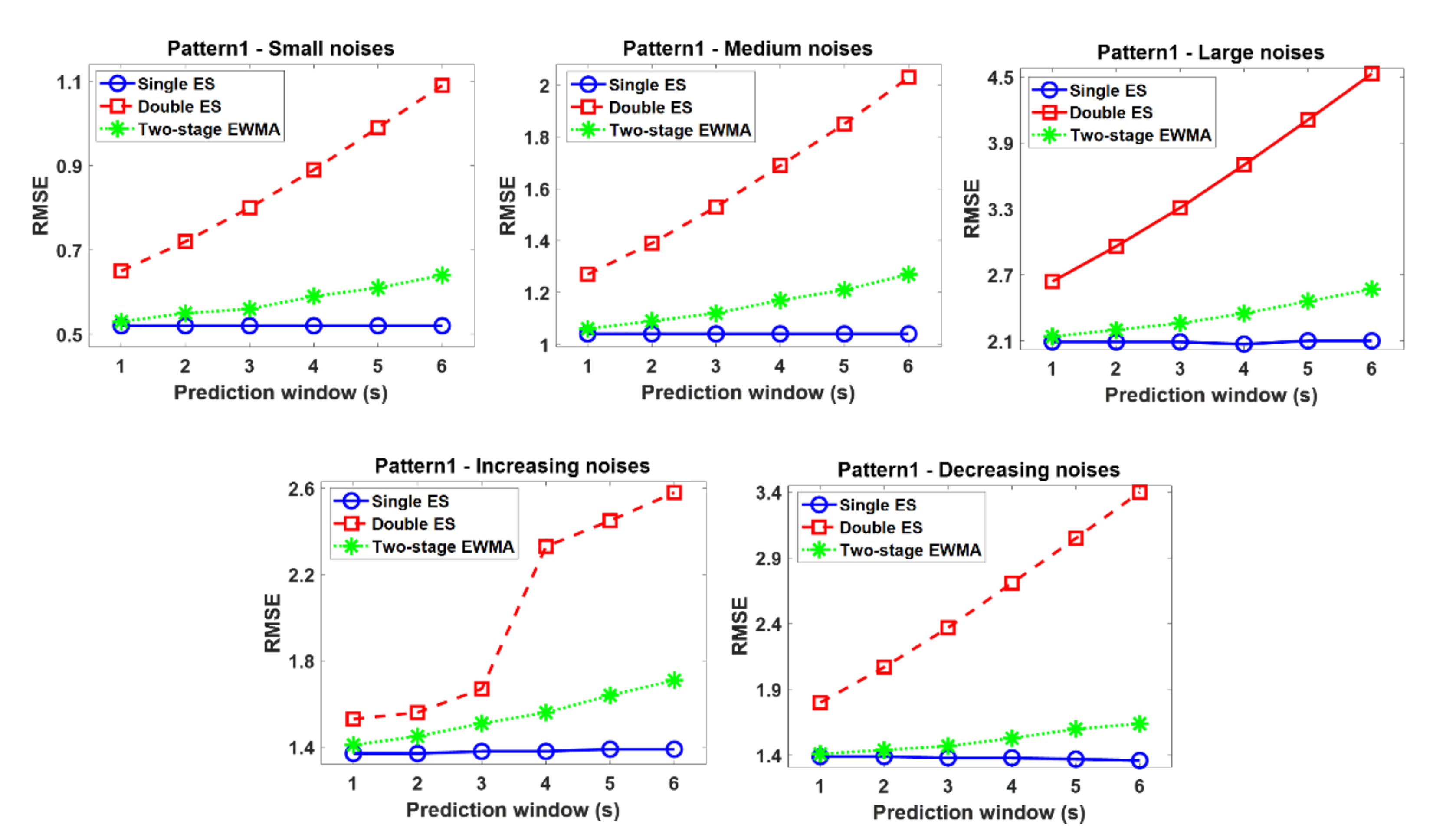
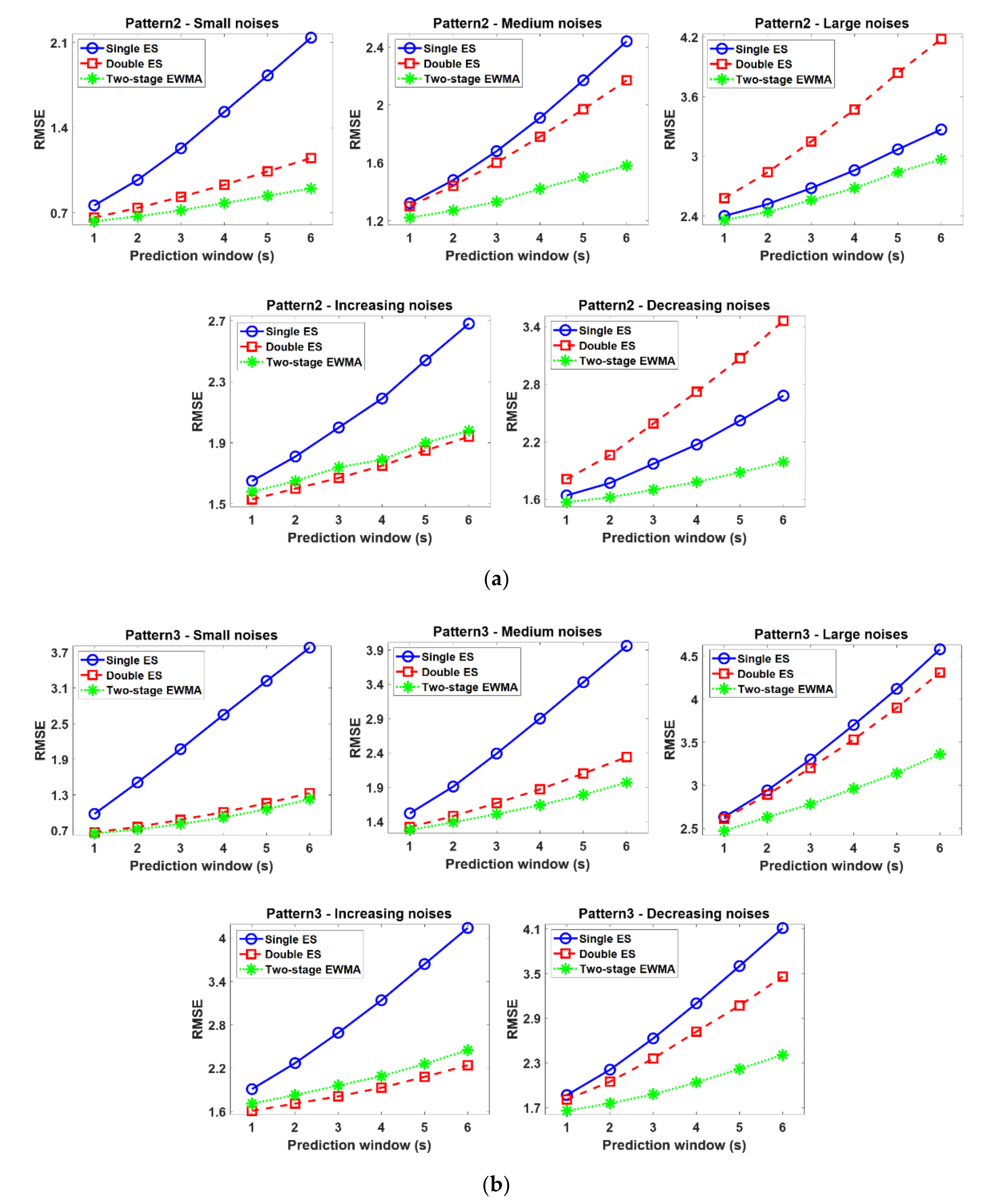
3.2. Simulation Results
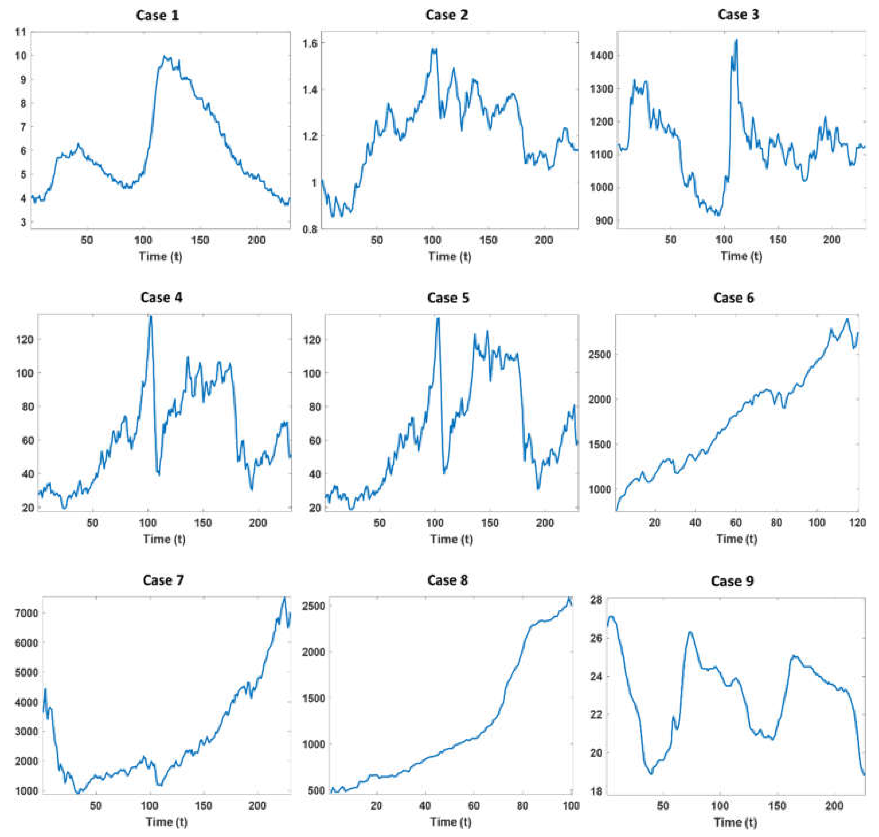
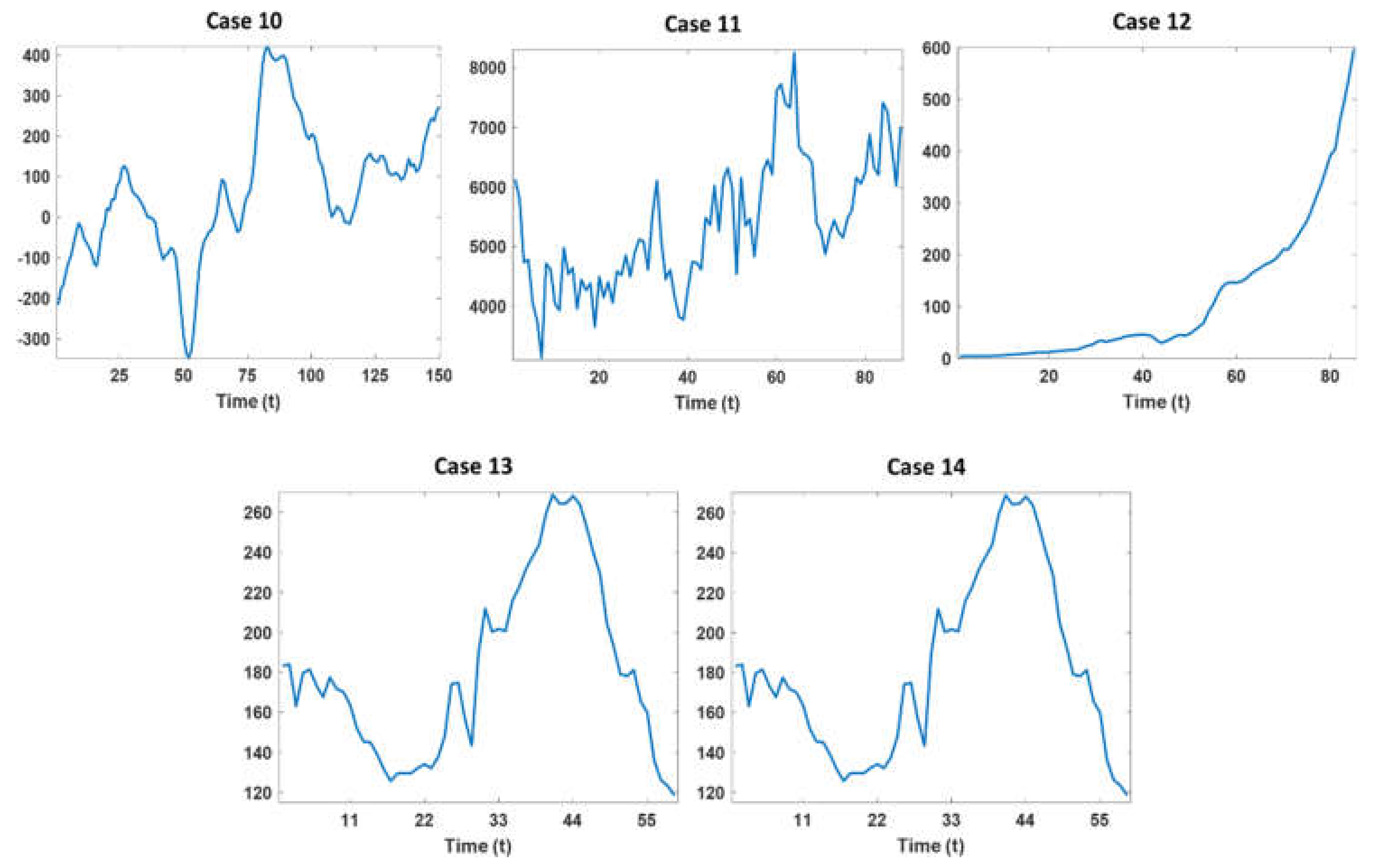
4. Case Study
5. Conclusions
- Single ES performs best only in the stationary time series and yields unsatisfactory results in nonstationary patterns. Thus, this model is not proper for the base model for the self-starting forecasting process in that, in many real situations, there is no assurance that the time series data is changed with stationary patterns.
- Double ES shows comparable or better performances than other EMWA models when the time series observations are monotonically increased or decreased. However, this model is vulnerable to the noises when there are no sufficient time series observations to compensate the effect of noise. In other words, the trend factor in the double ES model cannot be accurately estimated when large-sized noises are added to the insufficient time series observations, and these poorly estimated trend factors sequentially influence the successive model update process of the double ES model. Therefore, the double ES model might not be proper for a base model of the self-starting forecasting process in that the time series data in many real situations often contain large-sized noises.
- The seasonal factor in the triple ES model should be carefully estimated for the sake of more accurate forecasting. However, the seasonal factors are poorly estimated when the initial time series observations are not sufficient, and thus, the triple ES shows the worst performance although this model is designed for handling seasonality patterns. In addition, prior knowledge on the true period is not available when time series observations are not sufficiently accumulated. For these reasons, the tripe ES model is not appropriate to be used for a base model of the self-starting forecasting process.
- Conversely, the two-stage EWMA model tends to yield comparable or better performance than other EWMA models in all cases. In particular, this model outperforms other EWMA models as a base model for the self-starting forecasting process in the complex time series (i.e., non-stationary and noisy time series) because of the drift factor and adjustment factor. That is to say, the drift factor calculated as the first-order difference of two successive observations helps to accommodate the dynamics of the time series, and the adjustment factor helps to lessen the intrinsic bias caused by the noises and insufficient initial time series data. Finally, these appropriately estimated factors also lead to desirable EWMA model updates in the self-starting process.
Author Contributions
Funding
Conflicts of Interest
References
- Bowerman, B.L.; O’Connell, R.T.; Koehler, A.B. Forecasting, Time Series, and Regression: An Applied Approach; Thomson Brooks/Cole: Pacific Grove, CA, USA, 2005. [Google Scholar]
- Hunter, J.S. The Exponentially Weighted Moving Average. J. Qual. Technol. 1986, 18, 203–210. [Google Scholar] [CrossRef]
- Crowder, S.V.A. Simple Method for Studying Run Length Distributions of Exponentially Weighted Moving Average Control Charts. Technometrics 1987, 29, 401–407. [Google Scholar]
- Crowder, S.V. Design of Exponentially Weighted Moving Average Schemes. J. Qual. Technol. 1989, 21, 155–162. [Google Scholar] [CrossRef]
- Lucas, J.M.; Saccucci, M.S. Exponentially Weighted Moving Average Control Schemes: Properties and Enhancements. Technometrics 1990, 32, 1–12. [Google Scholar] [CrossRef]
- Friker, R.D.; Knitt, M.C.; Hu, C.X. Comparing Directionally Sensitive MCUSUM and MEWMA Procedures with Application to Biosurveillance. Qual. Eng. 2008, 20, 478–494. [Google Scholar] [CrossRef]
- Joner, M.D.; Woodall, W.H.; Reynolds, M.R.; Fricker, R.D.A. One-sided MEWMA Chart for Health Surveillance. Qual. Reliab. Eng. Int. 2008, 24, 503–519. [Google Scholar] [CrossRef]
- Han, S.W.; Tsui, K.-L.; Ariyajunyab, B.; Kim, S.B. A Comparison of CUSUM, EWMA, and Temporal Scan Statistics for Detection of Increases in Poisson Rates. Qual. Reliab. Eng. Int. 2010, 26, 279–289. [Google Scholar] [CrossRef]
- Snyder, R.D.; Koehler, A.B.; Ord, J.K. Forecasting for Inventory Control with Exponential Smoothing. Int. J. Forecast. 2002, 18, 5–18. [Google Scholar] [CrossRef]
- De Faria, E.L.; Albuquerque, M.P.; Gonzalez, J.L.; Cavalcante, J.T.P.; Albuquerque, M.P. Predicting the Brazilian Stock Market through Neural Networks and Adaptive Exponential Smoothing Methods. Expert Syst. Appl. 2009, 36, 12506–12509. [Google Scholar] [CrossRef]
- Rundo, F.; Trenta, F.; di Stallo, A.L.; Battiato, S. Machine Learning for Quantitative Finance Applications: A Survey. Appl. Sci. 2019, 9, 5574. [Google Scholar] [CrossRef]
- Jiang, H.; Fang, D.; Spicher, K.; Cheng, F.; Li, B. A New Period-Sequential Index Forecasting Algorithm for Time Series Data. Appl. Sci. 2019, 9, 4386. [Google Scholar] [CrossRef]
- Shilbayeh, S.A.; Abonamah, A.; Masri, A.A. Partially versus Purely Data-Driven Approaches in SARS-CoV-2 Prediction. Appl. Sci. 2020, 10, 5696. [Google Scholar] [CrossRef]
- Taylor, J.W. Short-term Electricity Demand Forecasting using Double Seasonal Exponential Smoothing. J. Oper. Res. Soc. 2003, 54, 799–805. [Google Scholar] [CrossRef]
- Brown, R.G. Exponential Smoothing for Predicting Demand; Arthur, D., Ed.; Little Inc.: Cambridge, MA, USA, 1956. [Google Scholar]
- Brown, R.G. Statistical Forecasting for Inventory Control; McGraw-Hill: New York, NY, USA, 1959. [Google Scholar]
- Holt, C.C. Forecasting Seasonals and Trends by Exponentially Weighted Moving Averages. Int. J. Forecast. 2004, 20, 5–10. [Google Scholar] [CrossRef]
- Winters, P.R. Forecasting Sales by Exponentially Weighted Moving Averages. Manag. Sci. 1960, 6, 324–342. [Google Scholar] [CrossRef]
- Box, G.E.; Jenkins, G.M.; Reinsel, G.C.; Ljung, G.M. Time Series Analysis: Forecasting and Control; John Wiley & Sons: Hoboken, NJ, USA, 2015. [Google Scholar]
- Akgiray, V. Conditional Heteroscedasticity in Time Series of Stock Returns: Evidence and Forecasts. J. Bus. 1989, 62, 55–80. [Google Scholar] [CrossRef]
- Sims, C.A. Macroeconomics and Reality. Econom. J. Econom. Soc. 1980, 48, 1–48. [Google Scholar] [CrossRef]
- Watson, M.W. Vector Autoregressions and Cointegration. Handb. Econom. 1994, 4, 2843–2915. [Google Scholar]
- Hochreiter, S.; Schmidhuber, J. Long Short-Term Memory. Neural Comput. 1997, 9, 1735–1780. [Google Scholar] [CrossRef]
- LeCun, Y.; Bengio, Y.; Hinton, G. Deep learning. Nature 2015, 521, 436–444. [Google Scholar] [CrossRef]
- Yang, H.; Pan, Z.; Tao, Q. Robust and Adaptive Online Time Series Prediction with Long Short-Term Memory. Comput. Intell. Neurosci. 2017, 2017, 1–9. [Google Scholar] [CrossRef] [PubMed]
- Divina, F.; Torres Maldonado, J.F.; García-Torres, M.; Martínez-Álvarez, F.; Troncoso, A. Hybridizing Deep Learning and Neuroevolution: Application to the Spanish Short-Term Electric Energy Consumption Forecasting. Appl. Sci. 2020, 10, 5487. [Google Scholar] [CrossRef]
- Hao, Y.; Gao, Q. Predicting the Trend of Stock Market Index Using the Hybrid Neural Network Based on Multiple Time Scale Feature Learning. Appl. Sci. 2020, 10, 3961. [Google Scholar] [CrossRef]
- Montgomery, D.C. Statistical Quality Control, 5th ed.; Wiley: New York, NY, USA, 2004. [Google Scholar]
- Ryu, E.S.; Han, S.W. The Slice Group Based SVC Rate Adaptation Using Channel Prediction Model. IEEE COMSOC MMTC E Lett. 2011, 6, 39–41. [Google Scholar]
- Ryu, E.S.; Han, S.W. Two-Stage EWMA-Based H.264 SVC Bandwidth Adaptation. Electron. Lett. 2012, 48, 127–1272. [Google Scholar] [CrossRef]
- Thomassey, S.; Fiordaliso, A. A Hybrid Sales Forecasting System Based on Clustering and Decision Trees. Decis. Support Syst. 2006, 42, 408–421. [Google Scholar] [CrossRef]
- Zou, C.; Zhou, C.; Wang, Z.; Tsung, F. A Self-starting Control Chart for Linear Profiles. J. Qual. Technol. 2007, 39, 364–375. [Google Scholar] [CrossRef]
- Hawkins, D.M. Self-starting CUSUM charts for Location and Scale. J. R. Stat. Soc. Ser. D 1987, 36, 299–316. [Google Scholar] [CrossRef]
- Menzefricke, U. Control Charts for the Variance and Coefficient of Variation Based on Their Predictive Distribution. Commun. Stat. Theory Methods 2010, 39, 2930–2941. [Google Scholar] [CrossRef]
- Linden, A.; Adams, J.L.; Roberts, N. Evaluating Disease Management Program Effectiveness: An Introduction to Time-Series Analysis. Dis. Manag. 2003, 6, 243–255. [Google Scholar] [CrossRef]
- Hyndman, R.J.; Kostenko, A.V. Minimum Sample Size Requirements for Seasonal Forecasting Models. Foresight 2007, 6, 12–15. [Google Scholar]
- Kang, J.H.; Yu, J.; Kim, S.B. Adaptive Nonparametric Control Chart for Time-varying and Multimodal Processes. J. Process Control. 2016, 37, 34–45. [Google Scholar] [CrossRef]


| Case | Duration of Time Series | Time Scale |
|---|---|---|
| Case 1: Unemployment rate in USA | 2000.01–2019.01 | Monthly |
| Case 2: USD–EUR exchange rate | 2000.01–2019.02 | Monthly |
| Case 3: USD–KRW exchange rate | 2000.01–2019.02 | Monthly |
| Case 4: WTI crude oil price | 2000.01–2019.01 | Monthly |
| Case 5: Brent crude oil price | 2000.01–2019.01 | Monthly |
| Case 6: S&P 500 index | 2009.01–2019.01 | Monthly |
| Case 7: NASDAQ-100 index | 2000.01–2019.02 | Monthly |
| Case 8: Australian expenditure on financial services | 1969.09–1994.03 | Quarterly |
| Case 9: Chemical process temperature readings | NA | Minute |
| Case 10: Changes in the Earth’s rotation day length | 1821–1970 | Yearly |
| Case 11: Total building and construction activities in Australia | 1973.09–1995.03 | Quarterly |
| Case 12: Money supply in USA | 1890–1974 | Yearly |
| Case 13: Birth per 10,000 of 23 year old people | 1961–2019 | Yearly |
| Case 14: Numbers on unemployment benefit in USA | 1984.01–2019.01 | Monthly |
| Case | EMWA Model | s = 1 | s = 2 | s = 3 | s = 4 | s = 5 | s = 6 | Average |
|---|---|---|---|---|---|---|---|---|
| Case 1 | Single ES | 0.17 | 0.26 | 0.35 | 0.44 | 0.53 | 0.62 | 0.40 |
| Double ES | 0.15 | 0.22 | 0.28 | 0.35 | 0.42 | 0.51 | 0.32 | |
| Two-stage EWMA | 0.15 | 0.21 | 0.28 | 0.33 | 0.39 | 0.47 | 0.31 | |
| Case 2 | Single ES | 0.03 | 0.05 | 0.06 | 0.07 | 0.08 | 0.09 | 0.06 |
| Double ES | 0.03 | 0.05 | 0.07 | 0.08 | 0.09 | 0.11 | 0.07 | |
| Two-stage EWMA | 0.03 | 0.05 | 0.06 | 0.07 | 0.08 | 0.09 | 0.06 | |
| Case 3 | Single ES | 28.46 | 45.93 | 57.41 | 66.86 | 76.29 | 85.51 | 60.08 |
| Double ES | 28.91 | 48.23 | 61.96 | 74.09 | 87.02 | 100.51 | 66.79 | |
| Two-stage EWMA | 25.48 | 45.35 | 56.37 | 65.63 | 73.43 | 82.76 | 58.17 | |
| Case 4 | Single ES | 5.74 | 9.35 | 12.37 | 14.78 | 16.78 | 18.39 | 12.90 |
| Double ES | 5.67 | 9.90 | 13.58 | 16.82 | 19.77 | 22.38 | 14.69 | |
| Two-stage EWMA | 5.08 | 8.34 | 11.46 | 13.77 | 15.59 | 17.54 | 11.96 | |
| Case 5 | Single ES | 5.92 | 9.58 | 12.50 | 14.81 | 16.75 | 18.42 | 13.00 |
| Double ES | 5.99 | 10.10 | 13.63 | 16.66 | 19.43 | 22.01 | 14.64 | |
| Two-stage EWMA | 5.33 | 8.95 | 11.86 | 14.41 | 16.09 | 17.86 | 12.42 | |
| Case 6 | Single ES | 53.49 | 80.72 | 99.46 | 115.55 | 129.62 | 144.23 | 103.85 |
| Double ES | 54.49 | 85.14 | 106.53 | 124.03 | 140.21 | 156.16 | 111.09 | |
| Two-stage EWMA | 49.47 | 76.97 | 93.08 | 105.16 | 114.09 | 122.17 | 93.49 | |
| Case 7 | Single ES | 151.05 | 230.85 | 289.31 | 340.43 | 390.81 | 442.15 | 307.43 |
| Double ES | 158.75 | 265.42 | 342.90 | 407.23 | 477.73 | 552.12 | 367.36 | |
| Two-stage EWMA | 139.70 | 222.72 | 275.33 | 321.19 | 361.35 | 402.55 | 287.14 | |
| Case 8 | Single ES | 40.40 | 67.80 | 96.53 | 125.10 | 153.53 | 181.59 | 110.83 |
| Double ES | 31.51 | 44.53 | 61.65 | 80.38 | 102.38 | 121.51 | 73.66 | |
| Two-stage EWMA | 29.64 | 41.23 | 56.46 | 72.36 | 91.03 | 107.80 | 66.42 | |
| Case 9 | Single ES | 0.25 | 0.46 | 0.66 | 0.85 | 1.03 | 1.19 | 0.74 |
| Double ES | 0.14 | 0.31 | 0.49 | 0.68 | 0.87 | 1.07 | 0.59 | |
| Two-stage EWMA | 0.14 | 0.28 | 0.44 | 0.60 | 0.76 | 0.92 | 0.52 | |
| Case 10 | Single ES | 29.57 | 53.40 | 74.62 | 92.72 | 108.53 | 122.14 | 80.16 |
| Double ES | 19.87 | 44.42 | 74.80 | 102.48 | 124.28 | 144.99 | 85.14 | |
| Two-stage EWMA | 17.46 | 36.79 | 60.13 | 81.02 | 98.35 | 111.90 | 67.61 | |
| Case 11 | Single ES | 599.66 | 713.71 | 805.95 | 853.11 | 1050.50 | 1049.90 | 845.47 |
| Double ES | 621.67 | 778.90 | 925.22 | 1047.40 | 1371.00 | 1546.80 | 1048.50 | |
| Two-stage EWMA | 608.68 | 721.59 | 795.26 | 777.03 | 998.28 | 1048.70 | 824.92 | |
| Case 12 | Single ES | 15.05 | 26.93 | 37.78 | 47.55 | 55.69 | 64.03 | 41.17 |
| Double ES | 5.70 | 10.40 | 16.23 | 22.91 | 25.54 | 31.73 | 18.75 | |
| Two-stage EWMA | 5.45 | 9.57 | 14.72 | 21.13 | 24.10 | 30.23 | 17.53 | |
| Case 13 | Single ES | 12.65 | 19.88 | 25.26 | 30.32 | 35.89 | 41.92 | 27.65 |
| Double ES | 12.05 | 18.28 | 22.11 | 26.27 | 32.51 | 40.55 | 25.30 | |
| Two-stage EWMA | 11.69 | 18.52 | 22.98 | 26.14 | 28.04 | 32.01 | 23.23 | |
| Case 14 | Single ES | 14404 | 24111 | 30938 | 36193 | 41164 | 46366 | 32196.00 |
| Double ES | 13835 | 23541 | 30264 | 35100 | 39573 | 44480 | 31132.17 | |
| Two-stage EWMA | 11485 | 22070 | 29333 | 33969 | 38237 | 42563 | 29609.50 |
Publisher’s Note: MDPI stays neutral with regard to jurisdictional claims in published maps and institutional affiliations. |
© 2020 by the authors. Licensee MDPI, Basel, Switzerland. This article is an open access article distributed under the terms and conditions of the Creative Commons Attribution (CC BY) license (http://creativecommons.org/licenses/by/4.0/).
Share and Cite
Yu, J.; Kim, S.B.; Bai, J.; Han, S.W. Comparative Study on Exponentially Weighted Moving Average Approaches for the Self-Starting Forecasting. Appl. Sci. 2020, 10, 7351. https://doi.org/10.3390/app10207351
Yu J, Kim SB, Bai J, Han SW. Comparative Study on Exponentially Weighted Moving Average Approaches for the Self-Starting Forecasting. Applied Sciences. 2020; 10(20):7351. https://doi.org/10.3390/app10207351
Chicago/Turabian StyleYu, Jaehong, Seoung Bum Kim, Jinli Bai, and Sung Won Han. 2020. "Comparative Study on Exponentially Weighted Moving Average Approaches for the Self-Starting Forecasting" Applied Sciences 10, no. 20: 7351. https://doi.org/10.3390/app10207351
APA StyleYu, J., Kim, S. B., Bai, J., & Han, S. W. (2020). Comparative Study on Exponentially Weighted Moving Average Approaches for the Self-Starting Forecasting. Applied Sciences, 10(20), 7351. https://doi.org/10.3390/app10207351