Automatic Classification of Text Complexity

Abstract

This work introduces an automatic classification system for measuring the complexity level of a given Italian text under a linguistic point-of-view. The task of measuring the complexity of a text is cast to a supervised classification problem by exploiting a dataset of texts purposely produced by linguistic experts for second language teaching and assessment purposes. The commonly adopted Common European Framework of Reference for Languages (CEFR) levels were used as target classification classes, texts were elaborated by considering a large set of numeric linguistic features, and an experimental comparison among ten widely used machine learning models was conducted. The results show that the proposed approach is able to obtain a good prediction accuracy, while a further analysis was conducted in order to identify the categories of features that influenced the predictions.

1. Introduction and Related Work

Natual language processing (NLP) is emerging in the recent years as one of hottest topics in the machine learning research community [1,2,3]. NLP tools are used and devised to tackle several real-world applications such as, just to name a few: automatic translation [4], text summarization [5], speech recognition [6], chatbots and virtual assistants [7], intelligent semantic search [8], sentiment analysis for social media [9,10], and product recommendations [11].

Another interesting application is to automatically classify a text according to its level of complexity from a linguistic point-of-view [12,13]. Text complexity measurement is key in a variety of applications such as: mood and sentiment analysis, text simplification, automatic translation, and also in the assessment of text readability in relation to both native and non-native readers.

In this work, we propose a text complexity classification tool built as a supervised learning system and trained by using a dataset of texts purposely collected and compiled by linguistic experts for second language learning purposes. In particular, the texts employed are taken from certification materials used for Italian language evaluation tasks. Therefore, such texts are implicitly categorized into different complexity levels according to the Common European Framework of Reference for Languages (CEFR) [14]. The goal was thus to design a supervised model to predict the CEFR level of any text written using the Italian language.

Such a proposal is important in the context of second language teaching and assessment. In fact, the suitability of a text for a certain learner group is generally established on the basis of its linguistic content, as it needs to be in line with the proficiency level of the learners. However, evaluations of the difficulty of a text are generally conducted subjectively, both when a text needs to be chosen as a component of a language test, and when it needs to be chosen for classroom use. The automatic classification system proposed in this work can introduce objectivity in these important teaching tasks.

In order to identify the objective characteristics of a text that make it difficult or easy to understand from a linguistic point-of-view, we design our system in such a way that any text is converted to a set of numeric values representing quantitative linguistic features calculated on, and extracted from, a given text. In fact, in the linguistic literature, the formal and quantitative characteristics of a text have a major role in determining the comprehensibility of that text, as they will impose specific cognitive demands upon the reader when approaching the text [15,16,17].

A number of research projects have been proposed with the aim of automatically assessing the difficulty of a text. Most of them involve the English language [18,19,20,21], though recent years have seen a rise of proposals involving languages other than English such as French [22], Swedish [23,24], Dutch [25], and Portuguese [26].

Flesch–Kincaid [20], Coh-metrix [21] and CTAP [18] are three of the most widely known automatic assessment systems for text difficulty, though all target the English language. In Italian, the three main approaches developed so far are: the Flesch–Vacca formula [27], the GulpEase index [28], and READ-IT [12]. From the computational point-of-view, the first two approaches are simple formulas involving the average length of words and sentences in terms of letters, syllables, or tokens, while READ-IT is based on a list of raw text, lexical, morpho-syntactic, and syntactic features, which are used to train a supervised statistical model that, in turn, allows us to produce a numeric assessment of an inputted text.

The main differences between the present work with the previous ones are: (i) the use of the CEFR levels as target classes in the classification system, (ii) a more extended set of numeric linguistic features, and (iii) a more thorough experimental comparison of different supervised classification models.

It is worthwhile to note that this article extends our preliminary works proposed in [29,30] and, to the best of our knowledge, it includes the most comprehensive set of linguistic features used to develop an automatic text classification system for the purposes of Italian language learning and teaching. In particular, with respect to [12,29], we include additional features such as discursive features as well as the recently introduced morphological complexity index [31]. Moreover, in [30] only the support vector machine model was investigated, while in this work we include a comprehensive comparison among ten different classification models widely used in the machine learning literature.

Importantly, note that neither this work nor the previously mentioned and related works consider the semantic content of a text as important for the task of measuring its linguistic complexity. In fact, a text can be linguistically difficult or easy independently from its semantic content. This aspect rules out the nowadays popular semantic methodologies like word and sentence embedding techniques [32,33,34] or most of the transfer learning approaches [35,36].

The rest of the article is organized as follows. Section 2 introduces the main architecture of the system, while Section 3 describes the collected dataset of texts. Text preprocessing operations are described in Section 4 and the features computation procedures are detailed in Section 5. The classification models adopted in this work are described in Section 6, where also the settings of their hyper-parameters are discussed. Experimental results are analyzed and discussed in Section 7. Finally, Section 8 concludes the article by outlining possible future lines of research.

2. Main Architecture of the Classification System

The task of measuring the complexity of a text is cast to a supervised classification problem by exploiting a dataset of texts purposely produced by linguistic experts for evaluating the language abilities of non-native speakers of Italian.

Interestingly, in 2001 the European Union introduced the Common European Framework of Reference for languages (commonly abbreviated as CEFR) [14] which recommends the use of a six-level scale in order to assess the language abilities of non-native speakers. Since then, the vast majority of institutions dealing with language teaching and assessment in Europe have adopted this scale. Hence, there is a large amount of texts used as assignments in language evaluation tasks which can be exploited in order to train a supervised classification model. The six CEFR levels, increasingly ordered by complexity, are: A1, A2, B1, B2, C1, and C2. However, in the language certification context, the texts used for the first two levels A1 and A2 are very short and elementary, thus practically useless for our purposes. For these reasons, our dataset was formed by collecting a corpus of texts used in the reading sections of language certification exams for the CEFR levels B1, B2, C1, and C2, which were manually labeled by language testing experts.

Using machine learning terms, we have a dataset of texts labeled with four different classes, which can be used to train a predictive model that, in turn, allows us to predict the complexity class of a previously unseen text.

As is common in the text classification field [37,38], we first convert any text into a numeric vector. This numeric representation allows us to directly use the most common models and algorithms available in the machine learning literature [39,40].

The numeric vector corresponding to a given text t is formed by the purposely defined quantitative linguistic features, which are computed from linguistic data structures obtained by running a natural language processing (NLP) pipeline on t. An NLP pipeline [41,42] includes a variety of processing steps (such as e.g., tokenization, part-of-speech tagging, and parsing) aiming at highlighting the linguistic structure of a text.

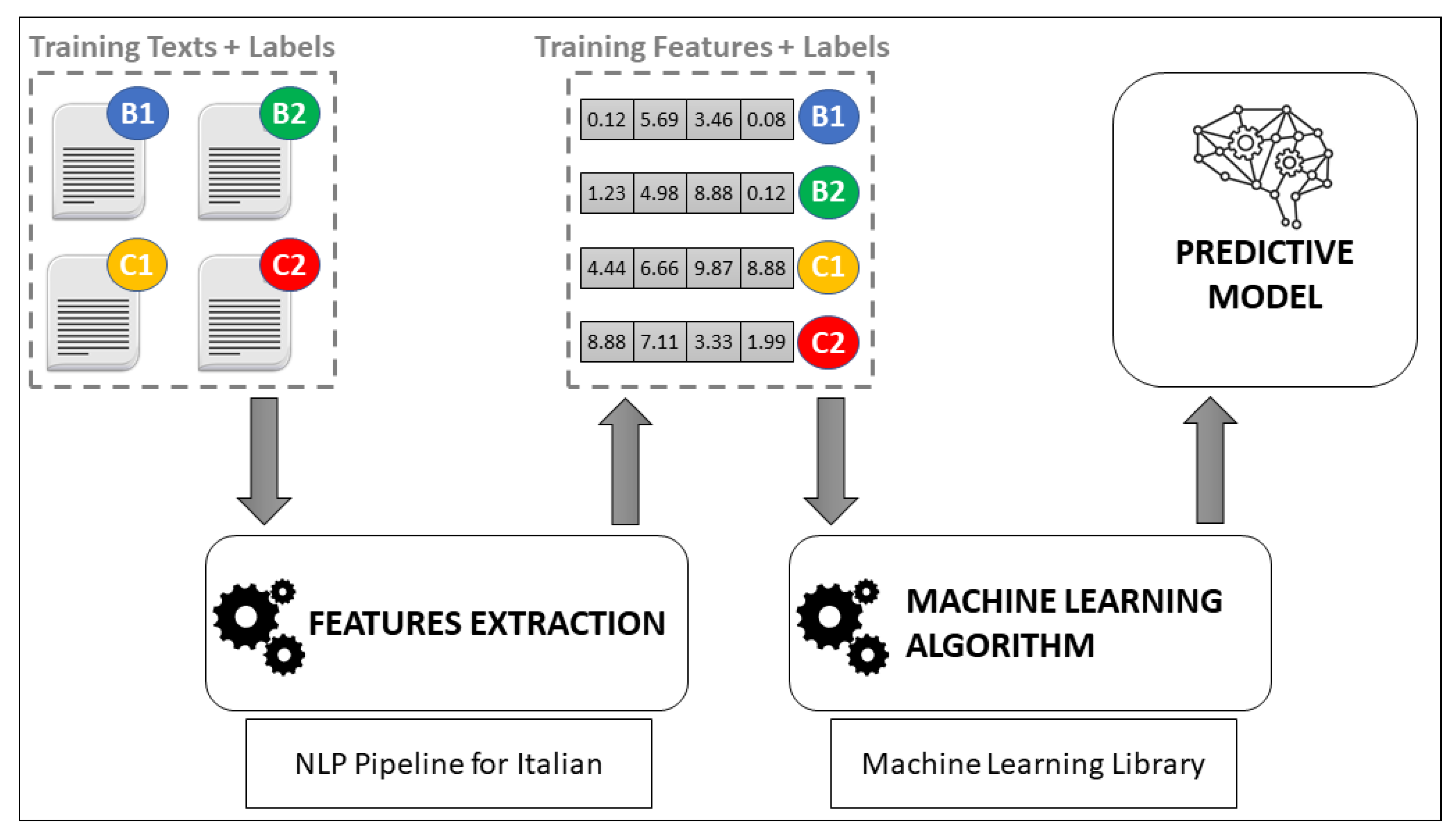
Hence, the working scheme of our classification system can be divided in two phases:

• the training phase, depicted in Figure 1, to be performed once (or sporadically, as new reliably labeled texts become available) and whose final goal is to train a predictive model by feeding a machine learning algorithm with a training set of numeric vectors obtained by extracting the linguistic features from the original dataset of texts correctly labeled by linguistic experts;
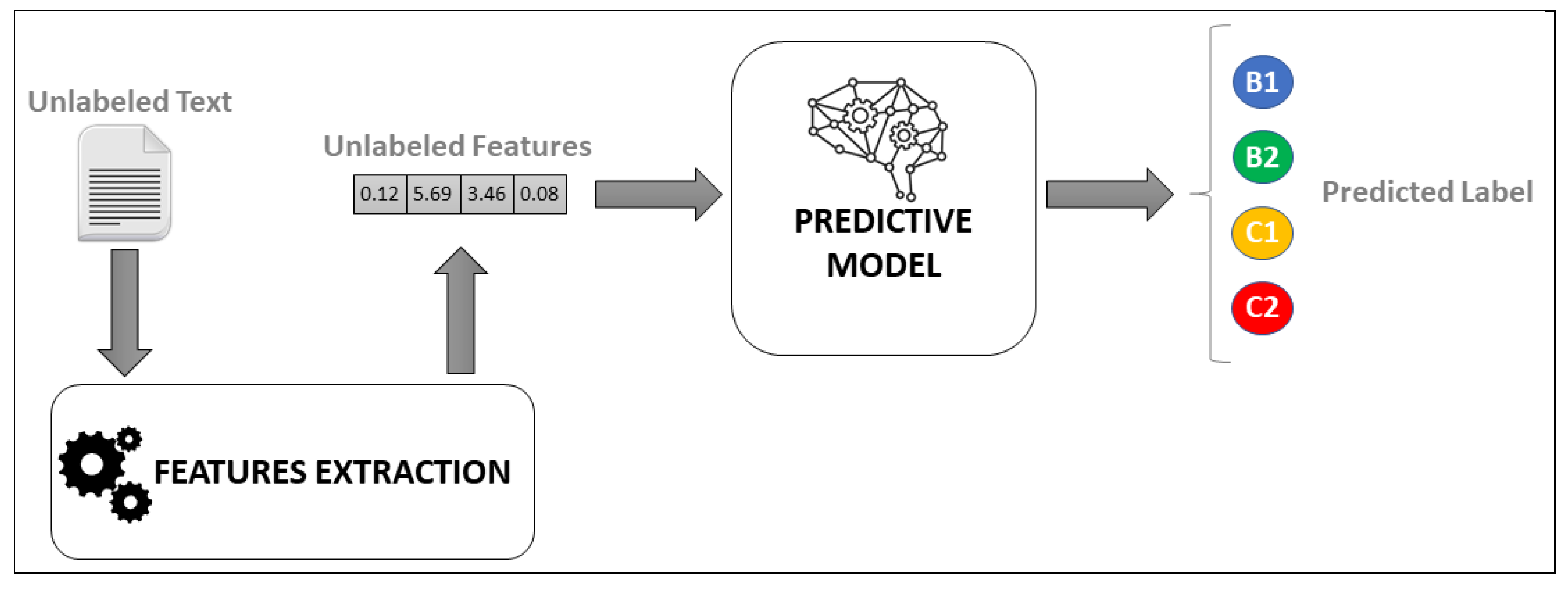
• the prediction phase, depicted in Figure 2, where an unlabeled text undergoes the process of features extraction and is then predicted to one of the four complexity levels B1, B2, C1, or C2.

Further details about the dataset, the NLP pipeline, the features extraction process, and the classification models adopted are provided in the following sections.

3. The Dataset of Italian Texts

The dataset is formed by a corpus of texts purposely identified, edited, or compiled by the linguistic experts of the center for language evaluation and certification (CVCL, i.e., Centro Valutazione Certificazioni Linguistiche) of the University for Foreigners of Perugia, one of the most recognized Italian language testing centers with sections spread all over the world.

The texts are taken from certification materials which have been used in a variety of Italian language evaluation tasks for the four CEFR levels B1, B2, C1, and C2. Therefore, for automatic classification purposes, we can state that any text in the considered dataset was manually labeled by domain experts to one of the four target classes B1, B2, C1, and C2. Moreover, a further validation of the class assignment is given by the fact that the texts were used in Italian language evaluation tasks carried out by a huge amount of learners worldwide.

The dataset is formed by 692 texts including a total of 336,022 tokens and 29,983 types (i.e., unique tokens throughout the entire dataset). The distribution of the texts among the four different classes is depicted in

Table 1. Characteristics of the dataset.

Class	#Texts	#Types	#Tokens
B1	249	7494	45,695
B2	185	12,743	90,133
C1	139	14,089	95,515
C2	119	15,709	104,679
Dataset	692	29,983	336,022

and it is slightly unbalanced.

In fact, the most represented class is B1 which accounts for roughly the 36% of the dataset, while the least represented class C2 corresponds to around the 17% of the texts. More generally, the number of texts per class decreases as the CEFR level increases. This may be due to the fact that there are generally more learners taking language certification exams at simpler levels, rather than more advanced ones.

Conversely, the number of tokens and types follow an opposite behavior: they increase together with the CEFR level. For instance, the class C2 accounts for roughly the 31% of the tokens in the entire dataset, more than the double of the tokens in B1, even though the texts in C2 are less than the half of those in B1. In fact, as we proceed from B1 to C2, we notice a steady increase in the number tokens and types and a steady decrease in the number of texts. This is a natural consequence of reading comprehension texts that, at higher proficiency levels, are longer and formed by a larger amount of different words [43,44,45].

4. NLP Pipeline for the Italian Language

An NLP pipeline is a library of computational tools which, given a plain text t in input, produce structured linguistic information about t in output. Most of the processing steps are organized in a pipeline fashion, i.e., the output of a generic processing step is usually fed in input to the next elaboration.

The different NLP pipeline libraries available [41,42,46,47,48] provide a variety of different functionalities. In our work, we are interested in the most basic lexical, morphological, and syntactic elaborations as briefly described in the following points:

• tokenization, which has the double goal of breaking the text into separate sentences and splitting any sentence into a list of tokens, i.e., words and punctuation marks;
• part-of-speech (POS) tagging, which marks every token with its POS category (noun, verb, adjective, adverb, etc.);
• lemmatization, which produces the lemma of every token, i.e., the canonical or base form of the word (e.g., infinite form for a verb, or singular and masculine form for a noun);
• analysis of the morphological features, whose goal is to provide a set of morphological annotations for every token (e.g., mood and tense of a verb, or gender and number of a noun);
• dependency parsing, which produces, for every sentence, its dependency tree, i.e., a tree data structure whose nodes are the tokens and the edges are labeled in order to highlight the syntactic dependency relations among the words (e.g., which noun is modified by an adjective, or which word is the subject of a verb);
• constituency parsing, which recursively divides up a sentence into its parts or constituents, thus producing a constituency tree whose root node is the full sentence, the inner nodes are meaningful chunks of the sentence (e.g., noun or verb phrases), and the leaf nodes are the single tokens.

For further details about automatic elaboration of natural language texts, the interested reader is referred to [49,50].

It is interesting to note that, in [51], a series of standard rules, guidelines, and formats have been defined in order to create cross-linguistically consistent lexical, morphological and syntactic annotations of a text. Since then, most of—though not all—the NLP pipeline libraries adhere to this standard.

The most modern NLP pipelines libraries rely on supervised statistical and machine learning models in order to produce the text annotations aforementioned. Therefore, their accuracy is highly dependent on the treebank corpus—as it is usually called, a manually annotated text corpus—adopted for training the predictive model. Moreover, note that a different treebank is required for any different language supported by an NLP pipeline library. This means that the Italian language is not as supported as e.g., the English language. Nevertheless, we have identified three modern NLP pipeline libraries which have predictive models for the Italian language: UDPipe [41], Spacy [46], and Tint [47]. After some preliminary experiments, we decided to choose UDPipe both because it resulted in a better accuracy on our experiments and because it is more adherent to standards defined in [51]. The version employed is the 2.5, i.e., the last stable UDPipe release at the time of writing.

Therefore, any text in our system was fed to UDPipe and the linguistic annotations produced were then used to compute the numeric features described in Section 5.

5. Numeric Linguistic Features

In our classification system, any text is converted to a numeric vector by computing a series of linguistic features on top of the data structures produced by UDPipe for the given text (see Section 4). Therefore, the features extraction process embeds the texts dataset in a multidimensial numeric space, where each dimension constitutes a linguistic feature purposely defined for discriminating the language complexity of the texts.

On the basis of a number of previous works [12,29,30,31,52,53,54,55,56,57]—in particular, those considering the readability of the Italian language [12,29,30,52]—we defined a set of 139 quantitative features. Therefore, any text is converted to a numeric vector in ${\mathbb{R}}^{139}$ so that the classification model will work exclusively with numeric data, without requiring it to handle textual data.

Note that the mapping from texts to vectors is not one-to-one, i.e., it may happen, though rarely, that multiple texts may be converted to the same vector. Anyway, since we are not interested in modeling or understanding the semantic meaning of the texts— let us recall that our only aim is to measure the language complexity of an Italian text—this does not constitute an issue for our purposes. It is indeed totally acceptable that two different texts have the same language complexity.

Hence, the chosen linguistic features are computed by means of purposely defined computation procedures which consider lexical, morphological, and syntactic aspects. For the same reason of above, semantic methodologies like the recently introduced word and sentence embedding techniques [32,33,34] are not considered in this work.

For the sake of presentation, we divide the 139 features into six categories, which are described in the following subsections.

5.1. Raw Text Features

Raw text features are the most elementary features used in this work and they are based on simple counting procedures executed on the tokenized text. They are briefly described in the following points.

• Number of sentences in the text, which gives a raw measure of how articulate is the text.
• Number of tokens per sentence: since a text is generally composed by multiple sentences, we register both the mean and standard deviation of the number of tokens per sentence.
• Number of characters per token: across all tokens in the text, we compute the mean and standard deviation of the token’s length in terms of characters.
• Number of different types in the text, i.e., the number of unique tokens in the entire text.

5.2. Lexical Features

The lexical features of a text are computed by considering: (i) the UDPipe elaborations for lemmas, POS tags and morphological annotations; (ii) two external and widely used resources for the Italian language such as [58,59]. The descriptions of all the lexical features used in this work are provided in the following points.

• Basic Italian vocabulary rate, which counts the number of lemmas of the given text belonging to the different categories of the Nuovo Vocabolario di Base della lingua Italiana (NVdB, which translates to “new basic Italian vocabulary”) [58], i.e., a widely used reference vocabulary for the Italian language, which provides a list of 7500 words classified for their usage level into the three categories: Fundamentals, High Usage, and High Availability. Therefore, the basic Italian vocabulary rate features are formed by three integers expressing the amounts of lemmas in the text falling into each one of the categories of the NVdB.
• Lexical diversity, i.e., the ratio between the number of types (unique tokens) and the number of tokens computed within 100 randomly selected tokens. As argued in [43], the randomly selected subset allows for a fairer comparison for texts of different lengths.
• Lexical variation features which include: (i) the lexical density [60], i.e., the ratio between content words—those tagged as verbs, nouns, adjectives, or adverbs—and the total number of words in a text; (ii) the distribution of the content words among each one of the four POS content categories (verbs, nouns, adjectives, and adverbs).
• Lexical sophistication, computed by considering the COLFIS lexical database [59] which provides a frequency lexicon for written Italian. Hence, lexical sophistication features are the mean and standard deviation of the COLFIS frequencies of the function tokens, function lemmas, lexical tokens, and lexical lemmas observed in the text.
• Nouns abstractness distribution [52], i.e., the percentages of noun tokens, which have been annotated in every one of the following three categories: Abstract, Semiabstract, and Concrete.

5.3. Morphological Features

In this work, we consider the morphological complexity index (MCI) [31] computed for two word classes: verbs and nouns.

The MCI is computed by the following procedure. First, a number of n samples, each one formed by k exponences (or inflectional forms), are randomly extracted from the given text for the considered word class. The average number of different exponences per sample is computed and used as a within-set diversity score. Moreover, an across-set diversity score is computed by: counting, for each pairs of samples, how many exponences belong to only one sample, and then averaging such counts. Finally, as depicted in [31], the MCI is computed by using the following formula

$$\mathtt{MCI}=\frac{\mathtt{within}-\mathtt{set}\mathtt{div}.+\mathtt{across}-\mathtt{set}\mathtt{div}.}{2}-1.$$

The values for the number of samples (n) and the sample dimensionality (k) have been set to, respectively, 100 and 10 as suggested in the MCI introductory article [31].

5.4. Morpho-Syntactic Features

Morpho-syntactic features are computed on the basis of POS tagging, morphological analysis, and parsing performed in the NLP pipeline elaboration. These features are largely used also in [12] and are briefly described in the following points.

• Subordinate ratio, i.e., the mean and standard deviation—computed across all the sentences in the given text—of the percentages of subordinate clauses over the total number of clauses.
• POS tags distribution, i.e., the percentage of tokens falling into every one of the POS categories defined in the universal dependencies standard [51]. Moreover, in order to include a measure of how spread is the distribution, we also computed its normalized entropy (i.e., the entropy divided by the maximum value it can achieve on the considered distribution).
• Verbal moods distribution, i.e., the percentage of verb tokens belonging to every one of the seven verbal moods (indicative, subjunctive, conditional, imperative, gerund, participle, and infinite). As for the POS tags, we also computed the normalized entropy of the verbal moods distribution.
• Dependency tags distribution, i.e., the percentage of dependencies—in the dependency tree—falling into every one of dependency categories defined in the universal dependencies standard [51]. As for the other categorical distributions considered in this work, the normalized entropy of the dependency tags distribution is computed.

5.5. Syntactic Features

The syntactic features reflect the main characteristics and the structure of the syntactic constituents and the dependency relations of the sentences that form the given text. These features are widely used also in [12,18] and are described in the following points.

• Depth of the dependency trees: by noting that a dependency tree is created for each sentence in the given text, this feature is the maximum depth among all the dependency trees.
• Length of non-verbal chains, i.e., the mean and standard deviation of the lengths of the maximal-length paths without verbal nodes in all the dependency trees.
• Verbal roots, i.e., the percentage of dependency trees with a verbal root.
• Arity of verbal predicates, i.e., the distribution of the arity of the verbal nodes in all the dependency trees, where the arity is the number of dependency links involving the verbal node as head. After few preliminary experiments, we decided to maintain a discrete distribution of the arities by registering the percentage of verbal nodes with 1, 2, 3, 4, and ≥5 links.
• Length of the dependency links: given a dependency link between two tokens, its length is the number of words between the two tokens occurring in the usual linear representation of the sentence. We aggregate the lengths of all the dependency links by maintaining the mean, the standard deviation, and the maximum length.
• Maximal non-verbal phrase, which is computed on the basis of the constituent trees of every sentence in the given text by: taking all the subtrees that are nominal phrases (NP) and are not contained in larger NP subtrees, counting how many leaf nodes (i.e., tokens) they contain, and computing the mean and standard deviation of such quantities.
• Number of syntactic constituents, i.e., the counts of the occurrences of specific syntactic constituents in the text. The following elements are considered: clauses, nominal phrases, coordinate phrases, and subordinate clauses.
• Syntactic complexity, which is given by three indices [61]: the average number of coordinate phrases per clause; the sentence complexity ratio (i.e., the ratio between the number of clauses and the number of sentences); the sentence coordination ratio (i.e., the ratio between the number of coordinating clauses and the number of sentences).
• Relative subordinate order, i.e., the distribution of the distances between the main clause and each subordinate clause. After few preliminary experiments, we decided to maintain a discrete distribution of the distance values by registering the percentage of subordinate clauses at distance 1, 2, 3, 4, and ≥5 from the main clause.
• Length of clauses, which is represented by the mean and standard deviation of the lengths of all the clauses expressed in number of tokens.
• Subordination chains length, i.e., the distribution of the depth of chains of embedded subordinate clauses. As for the other integer distributions considered in this section, we maintain counts for depth values of 1, 2, 3, 4, and ≥5.

5.6. Discursive Features

The discursive features takes into account the cohesive structure of the text [21,52]. They are summarized in the following points.

• Referential cohesion is represented by the mean and standard deviation of the number of nominal types, which appear in more adjacent sentences up to length 3. Further linguistic considerations about the referential cohesion are provided in [52].
• Deep causal cohesion, i.e., the distribution of the eight classes of connectives—causal, temporal, additive, adversative, marking results, transitions, alternative, and reformulation/ specification—and its normalized entropy. These features play an important role in the creation of logical relations within text meanings and are further discussed in [52].

6. Classification Models

Since the text dataset is converted to a multi-dimensional numeric dataset by computing the linguistic features of every text, it is now possible to adopt the most popular classification models and training algorithms available in the machine learning literature [39,62].

In order to validate our approach for the classification of the complexity of an Italian text, we conducted an extensive experimental comparison by training and evaluating 10 classification models on the dataset previously described. The implementations provided in the popular Sci-kit Learn library [40] (version 0.23, the last stable release at the time of writing) were used in this work.

Moreover, before training the classification models, the numeric dataset was normalized in order to bring the different features to a common and comparable scale, thus avoiding possible biases due to the different ranges of the different features. Hence, we have executed a standardization procedure independently on every feature dimension, i.e., every feature value x is transformed to $\frac{x-m}{q_3-q_1}$, where m, $q_1$ and $q_3$ are, respectively, the median, first, and third quartiles for the given feature on the considered dataset. This procedure is known to be robust to outliers [39] and it was chosen because we have observed some outlier values in few features of our numeric dataset.

The 10 classification models considered in this work are listed in

Table 2. Classification models considered in this work.

Model	Description
RF	Random Forest classifier
GBDT	Gradient Boosted Decision Tree classifier
SVM	Support Vector Machine with radial basis function as kernel
MLP1	Multi-Layer Perceptron with one hidden layer
MLP2	Multi-Layer Perceptron with two hidden layers
MLP3	Multi-Layer Perceptron with three hidden layers
QDA	Quadratic Discriminant Analysis classifier
NB	Naive Bayes classifier which fits Gaussian distributions
kNNU	K-Nearest Neighbors with uniform weights
kNND	K-Nearest Neighbors with weights set on the basis of the distance in the features space

and briefly described in the following together with their settings. For the parameters not mentioned in the descriptions, we have adopted the default values as set in the Sci-kit Learn library.

The random forest (RF) [63] and gradient boosted decision tree (GBDT) [64] are two ensemble-based classification models that train multiple weak decision tree classifiers and compose their predictions. RF uses the so-called bagging technique [39], while GBDT is based on the boosting process [39]. Practically, RF trains multiple decision trees simultaneously, each one on a different random sample of the dataset, and then averages their predictions. Instead, GBDT sequentially trains a series of decision trees, each one on the residual error function of the previous tree, thus building an additive loss function that is minimized by means of a gradient descent algorithm. After some preliminary experiments (see also [29]), we used 100 weak decision tree estimators with a maximum depth equal to the integral part of the square root of the number of features (in our work: $\lfloor \sqrt{139}\rfloor =11$).

The support vector machine (SVM) model [65] aims at constructing a set of hyperplanes in a high-dimensional space in order to separate the regions of the space corresponding to sample instances from the different classes (i.e., the CEFR levels in our case). A higher dimensional space is implicitly induced by a non-linear kernel function that, in our case, is the commonly adopted radial basis function. Further parameters that weigh the regularization penalty and the influence of the training instances on the decision surface are, respectively, C and $\gamma$ that, in our preliminary work [30], have been experimentally tuned to $C=2.24$ and $\gamma =0.02$.

The multi-layer perceptron (MLP) [62] is the classical feed-forward neural network, which is a prediction model organized in different layers of so-called artificial neurons: the first—or input—layer is formed by the 139 numeric features considered in our work, the last—or output—layer produces an estimated output value for every one of the four target classes considered (i.e., the CEFR levels), while one or more inner—or hidden—layers allow us to learn a mapping from the input to the output. Any artificial neuron is connected to all the neurons in the previous layer, all the connections have a weight, and the output of a neuron is a non-linear combination of its weighted input values. Hence, a gradient descent algorithm is used to learn the network’s weights and minimize a loss function on the given training set. In this work we considered three MLP models: MLP₁ is a shallow neural network with only one hidden layer, MLP₂ uses two hidden layers, while MLP₃ is the deeper neural network here considered which has three hidden layers. After some preliminary experiments, we chosen the following setting: 25 artificial neurons for each hidden layer, the relu as activation function, the cross-entropy as loss function, and the popular Adam variant of the stochastic gradient descent algorithm.

The quadratic discriminant analysis (QDA) [66] and the naive Bayes (NB) [67] are two classifiers based on Bayesian probability theory [62]. QDA learns, for each target class, a multivariate Gaussian probabilistic model of the class conditional distribution on the given training set. Then, predictions are obtained using the Bayes rule and selecting the class that maximizes the posterior probability. Note that, QDA was preferred to its linear counterpart after performing some preliminary experiments. Regarding the NB classifier, it learns a simplified Bayesian network model of the given training set and uses the learned model to perform probabilistic predictions. Since in this work we are considering a real-valued dataset, the Gaussian-based NB model was adopted. Hence, it is interesting to note that, under this setting, NB can be seen as a simplified version of QDA where the learned covariance matrices are diagonal.

The last method considered is K-nearest neighbors (kNN) [68], which does not learn a proper model of the class distributions but, conversely, memorizes the training set and performs predictions by outputting the most common target class among the k nearest training vectors to the (unlabeled) query vector. Therefore, kNN training only consists in organizing the training vectors in a suitable data structure for speeding up the computation of the k nearest vectors in the prediction phase [69]. This method was used in this work because our dataset is not huge. Moreover, two different variants of kNN were considered: kNN_U and kNN_D. In kNN_U all the neighbors count equally, while in kNN_D their votes are weighted by the inverse distance from the query vector. We used the classical Euclidean distance function and, after some preliminary experiments, we set the number of neighbors k to 7.

7. Experiments

In order to assess the effectiveness of the proposed approach and to compare the ten classification models described in Section 6, a number of experiments were held by using the dataset of 692 texts described in Section 3.

In particular, two main experiments were held. First of all, we experimentally compared the classification models by considering the whole set of 139 features described in Section 5. This allows us to use most of the informative content of the texts, but the results may suffer the curse of dimensionality, due to the not very large ratio between dataset size and number of features. For this reason, a second experiment was held by executing a preliminary features selection phase aiming at reducing the vectors dimensionality by removing those features that do not show to be statistically relevant for classification accuracy.

Both experiments were designed as a stratified 10-folds cross-validation process repeated 25 times. The significance of the experimental results is also analyzed by means of non-parametric statistical tests. The experimental comparison among the classification models is described in Section 7.1, while the experiment involving the features selection procedure is analyzed in Section 7.2. Finally, in Section 7.3 we provide a detailed analysis of the results obtained by the most performing (considering both experiments) classification model.

7.1. Experimental Comparison Considering All the Features

For any prediction model, the averaged results of the 25 cross-validation repetitions are provided in

Table 3. Averaged results for the experiment that considers all the features.

Model	Accuracy	Precision	Recall	F1 Score
RF	0.725 =	0.696	0.691	0.694
SVM	0.717 =	0.690	0.682	0.686
MLP3	0.684 ▾	0.663	0.657	0.660
MLP2	0.674 ▾	0.657	0.653	0.655
GBDT	0.667 ▾	0.634	0.634	0.634
MLP1	0.651 ▾	0.625	0.624	0.624
NB	0.597 ▾	0.568	0.580	0.574
kNNU	0.542 ▾	0.560	0.541	0.550
kNND	0.530 ▾	0.551	0.537	0.544
QDA	0.415 ▾	0.442	0.318	0.369

by considering four metrics: classification accuracy, macro-averaged precision, recall, and F1 score. The models are ordered by accuracy.

First of all, let us note that: the ranking among the models is stable across all the four metrics, and the difference between accuracy and F1 scores is small. These two observations suggest that the slight imbalance of the dataset does not constitute a big issue in practical terms.

In order to further analyze the results of Table 3, let us also consider the baseline classification rule ZeroR, which always outputs the most frequent dataset class [39]. By considering the data in Table 1, ZeroR has an accuracy of 0.36, larger than that of a totally random classifier (0.25). Interestingly, all the models involved in our comparison obtained better accuracy scores with respect to ZeroR, thus validating our general approach.

Nevertheless, important differences in terms of effectiveness can be observed among the models for all the considered metrics. The best performing models are RF and SVM, which correctly classified, respectively, 72.5% and 71.7% of the dataset. They both outperformed the neural network models MLP₃, MLP₂, MLP₁, and the other tree-based model GBDT, that were able to reach an accuracy larger than 0.65. Further, the two kNN variants and the Bayesian models NB and QDA had an accuracy smaller than 0.60. In particular, the last one is better than ZeroR by only five percentage points, thus revealing that QDA is possibly overfitting the training set.

In order to statistically analyze the differences between the best performing model RF and all the rest of the models, we conducted the non-parametric Mann–Whitney U test [70] on the accuracy scores obtained by the 25 repetitions of the cross-validation experiment. Therefore, by considering a significance level of 0.05, in Table 3, beside the accuracy scores of every model (except RF), we mark with the symbol “=” the models that are statistically equivalent to RF, and with the symbol “▾” those models that are significantly outperformed by RF. The marks in Table 3 show that the only model that is not significantly outperformed by RF is SVM—with a small p-value of around 0.09,—while all the other models are significantly outperformed and registered a p-value smaller than ${10}^{-5}$.

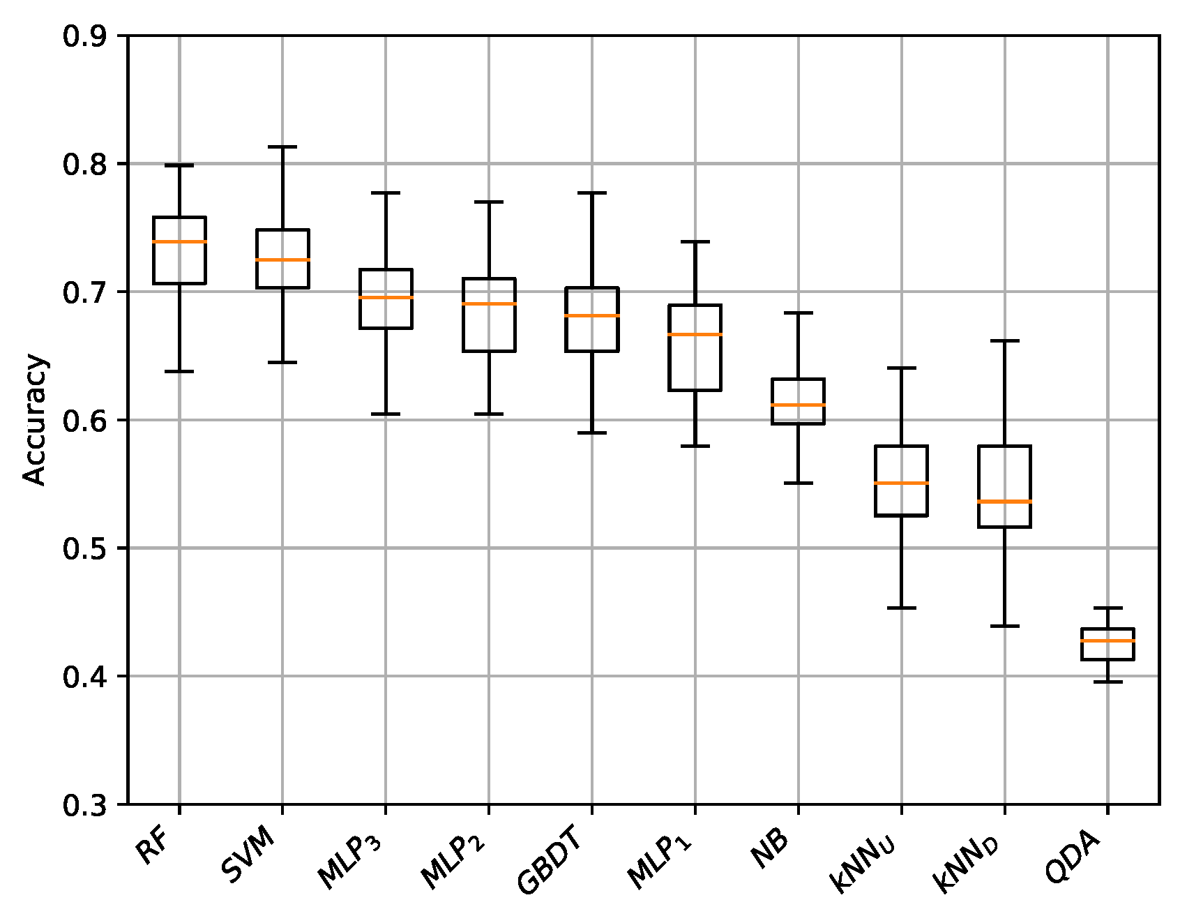
Finally, in Figure 3, we provide the box-plots for the accuracy scores obtained by all the models in the 25 repetitions of the cross-validation experiment. Interestingly, the small size of the boxes show a good robustness for the proposed approach. Numerically, the larger standard deviation among the 25 accuracy scores is only 0.044 and it was observed for the two kNN models, while the most performing RF model registered a smaller standard deviation of 0.036. Moreover, let also note that the repetition with the best accuracy was obtained by the SVM model.

7.2. Experimental Results with Features Selection

A further experiment was held by executing a preliminary features selection procedure in order to reduce the dimensionality of the numeric vectors and make the prediction model focus on the most informative linguistic features.

The features selection was performed by means of the well known recursive features elimination (RFE) algorithm [71]. The RFE algorithm recursively fits the model, ranks the features according to a measure of their relevance to the classification process, and finally removes the weakest one. For the tree-based models RF and GBDT, the features importance is calculated as the Gini importance index [72], while for the rest of the models we used the well known permutation features importance technique [73]. Moreover, to find the optimal number of features, RFE was cross-validated in order to score feature subsets of different sizes.

For each model, the number of features selected is provided in

Table 4. Amount of selected features per model.

	RF	SVM	MLP3	MLP2	MLP1	GBDT	kNNU	kNND	QDA	NB
Number of sel. features	58	54	53	51	53	59	48	50	60	62
Percentage of sel. features	41.7%	38.8%	38.1%	36.7%	38.1%	42.4%	34.5%	36.0%	43.2%	44.6%

. Interestingly, the number of selected features does not vary greatly across the different models and it ranges from 48 (kNN_U) to 62 (NB). Hence, more than half of the totality of the features is removed by RFE. Furthermore, the set of selected features is quite stable among the different models.

Hence, all the classification models considered in this work were analyzed using the reduced sets of features identified by the features selection procedure. The accuracy scores of the cross validation process are provided in

Table 5. Average accuracy scores for the experiment with features selection.

	RF	SVM	MLP3	MLP2	MLP1	GBDT	kNNU	kNND	QDA	NB
Accuracy	0.741	0.727	0.688	0.680	0.674	0.670	0.646	0.643	0.631	0.627
Improvement	+0.016	+0.010	+0.004	+0.006	+0.023	+0.003	+0.104	+0.113	+0.216	+0.030
Significance	=	=	=	=	▴	=	▴	▴	▴	▴

, together with the improvement of accuracy with respect to the experiment analyzed in Section 7.1 and a symbol that indicates if the improvement is statistically significant or not (the symbol “=” indicates no difference with the previous experiment, while “▴” and “▾” indicate that the new execution, respectively, significantly outperforms or is significantly outperformed by the previous one). The statistical test considered is the Mann–Whitney U test with a significance threshold of 0.05.

The models in Table 5 are ordered (from left to right) by accuracy. RF, as in the previous example, is the model showing the larger accuracy, 74.1%, which improves the previous experiment by 1.6%. This improvement is not statistically significant, though the p-value of the statistical test, 0.08, is close to the significance threshold. Overall, all the models show an improvement of accuracy with respect to the previous experiment. The improvement is statistically significant for MLP₁, kNN_U, kNN_D, QDA, and NB. It is interesting to observe the large improvement for the two kNN schemes observed using the features space with reduced dimensionality. By recalling that kNN works by computing distances in the features space, the improvement in accuracy can be interpreted as the fact that the removed features were, in some sense, spatially misleading.

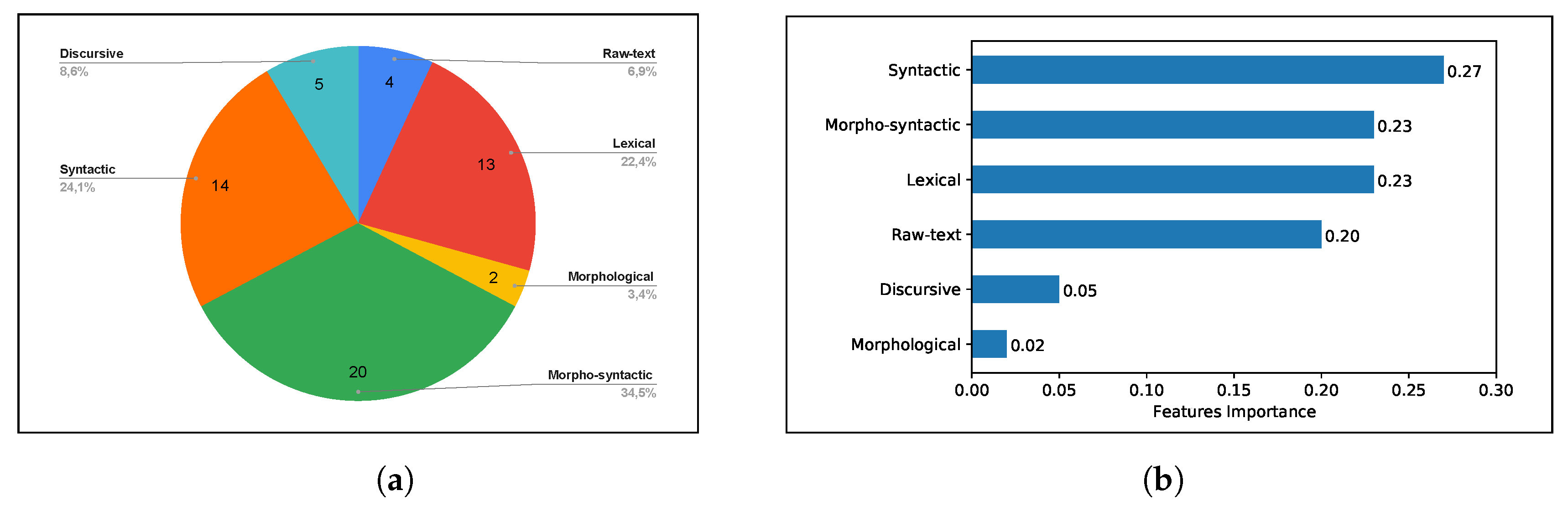
Finally, we analyze the selected features by considering the best performing model RF. Figure 4a shows the distribution of the selected features within each feature category (see Section 5). As we can see, morpho-syntactic, syntactic, and lexical features constitute the categories with most features represented in the final set. Furthermore, in Figure 4b, we provide the normalized Gini importance indices—summed up for each category of features—of the RF model. Figure 4b shows that the most impactful features are in the three most selected categories (syntactic, morpho-syntactic, and lexical) and the raw-text features. In particular, let us note that, though only four raw-text features were selected (Figure 4a), they have a very similar Gini importance with respect to the top three categories. Overall, the syntactic features look to have the highest discriminating power.

Finally, it is important to highlight that some additional experiments were performed by asking linguist experts to feed the system with: (i) very long B1 texts of about 5000 words, and (ii) very short C2 texts of about 500 words. Interestingly, both types of texts were correctly classified, thus showing that the proposed system is more effective and, in some sense, more intelligent than a silly classification only based on the length of the text in input.

7.3. Analysis of the Experimental Results for the Random Forest Model

The best classification accuracy (0.741) was obtained by the random forest (RF) model executed on a smaller set of features as described in Section 7.2.

Here, we provide a further analysis of this result by showing, in

Table 6. Confusion matrix for the random forest (RF) model with features selection.

Pred.	B1	B2	C1	C2
Actual
B1	222.7	26.1	0.1	0.0
B2	26.3	140.9	17.6	0.1
C1	0.3	45.8	58.9	34.0
C2	0.0	0.5	28.1	90.4

, the confusion matrix of the experiment. In this table, each entry $X,Y$ indicates the average number—over the 25 repetitions of the 10-folds cross-validation process—of texts which are known to belong to the CEFR level X, but have been classified to the CEFR level Y by the RF model.

The correctly classified texts are those accounted in the diagonal of the confusion matrix. In average, 512.9 out of 692 texts were correctly predicted, thus confirming the average accuracy of 74.12%. The confusion matrix also allows us to derive precision and recall measures [39] for all the considered target classes. Observing the data, it is possible to see that the B1 class exhibits the highest precision and recall—respectively, 89.33% and 89.47%—while the weakest predictions are those involving the C1 class, with 56.26% precision and 42.37% recall.

Furthermore, let observe that most of the incorrectly classified texts are only one level away from their actual classes, i.e., the non-diagonal entries of the confusion matrix showing larger values are those adjacent to the main diagonal. In average, only one text out of 692 was classified to a CEFR class distant two or three levels from the actual class of the text. Therefore, the errors produced by our approach are, in some sense, small errors. This is an interesting aspect, especially in light of the fact that, in order to use the most common prediction models in the machine learning literature, we are not considering at all the intrinsic ordering among the four CEFR classes.

Another important observation is that, often in the linguistic field, the pairs of CEFR levels B1, B2 and C1, C2 are aggregated into the macro-levels B and C, respectively. By considering this aggregation and the data provided in Table 6, it is possible to see that the average accuracy of our system increases up to the remarkable percentage of 90.66%.

Finally, note that the results discussed are also in line with the 2D visualizations of the dataset depicted in Figure 5, which provides the results of two different executions of the well known stochastic dimensionality reduction technique t-SNE [74] executed on the 139-dimensional representation of the dataset. Every point in the visualizations is the two-dimensional representation of a text in the dataset, while its color indicates the CEFR class of the text. According to t-SNE working principles [74], the spatial distances among the points indicate how distant are the corresponding text in terms of numeric features, thus how easy or difficult is to discriminate the CEFR classes. Clearly, both visualizations show that B1 is the easier class to discriminate, while C1 and C2 are the more difficult to discern.

8. Conclusions and Future Work

In this work we have introduced a computational system for automatically classifying Italian written texts according to their difficulty. A web-based interface is made publicly available at this URL: https://lol.unistrapg.it/malt.

CEFR levels were considered as target classes of the classification system, thus allowing us to reuse the teaching and assessment materials adopted for second language learning purposes in order to train a prediction model. A wide set of quantitative linguistic features were considered and computational procedures were devised in order to extract numeric features from a given text. Therefore, the linguistic features allowed us to vectorize the texts, so that the most common machine learning models can be used.

Experiments were held in order to analyze the effectiveness and the reliability of the proposed classification system. In particular, ten different classification models from the machine learning literature were considered. Overall, the experimental results indicate that the proposed approach reaches a very good accuracy level, in particular when the random forest model is considered.

Furthermore, indications regarding which features are more important in the classification process are provided. In particular, this latter point paves the way for an interesting direction for future works aiming at objectively modeling the linguistic aspects that make a text difficult or easy to understand. Another interesting point in this direction is also a possible contrastive and quantitative analysis in the features space of corpora belonging to different languages.

Finally, from a computational point-of-view, interesting future lines of research regard: the use of semantic features [75,76] for the task analyzed in this article, the automatic augmentation of a text dataset used, not for semantic, but syntactic and linguistic tasks, and the use of evolutionary search techniques (such as [77,78,79,80]) for automatically tuning the classification engine without any manual intervention.

References

- Schmidt, A.; Wiegand, M. A survey on hate speech detection using natural language processing. In Proceedings of the Fifth International Workshop on Natural Language Processing for Social Media, Valencia, Spain, 3 April 2017; pp. 1–10. [Google Scholar]
- Goldberg, Y. Neural network methods for natural language processing. Synth. Lect. Hum. Lang. Technol. 2017, 10, 1–309. [Google Scholar] [CrossRef]
- Young, T.; Hazarika, D.; Poria, S.; Cambria, E. Recent trends in deep learning based natural language processing. IEEE Comput. Intell. Mag. 2018, 13, 55–75. [Google Scholar] [CrossRef]
- Vaswani, A.; Bengio, S.; Brevdo, E.; Chollet, F.; Gomez, A.; Gouws, S.; Jones, L.; Kaiser, Ł.; Kalchbrenner, N.; Parmar, N.; et al. Tensor2Tensor for Neural Machine Translation. In Proceedings of the 13th Conference of the Association for Machine Translation in the Americas (Volume 1: Research Papers), Boston, MA, USA, 17–21 March 2018; pp. 193–199. [Google Scholar]
- Gambhir, M.; Gupta, V. Recent automatic text summarization techniques: A survey. Artif. Intell. Rev. 2017, 47, 1–66. [Google Scholar] [CrossRef]
- Afouras, T.; Chung, J.S.; Senior, A.; Vinyals, O.; Zisserman, A. Deep audio-visual speech recognition. IEEE Trans. Pattern Anal. Mach. Intell. 2018. [Google Scholar] [CrossRef] [PubMed]
- Dale, R. The return of the chatbots. Nat. Lang. Eng. 2016, 22, 811–817. [Google Scholar] [CrossRef]
- Bast, H.; Björn, B.; Haussmann, E. Semantic search on text and knowledge bases. Found. Trends Inf. Retr. 2016, 10, 119–271. [Google Scholar] [CrossRef]
- Cambria, E. Affective computing and sentiment analysis. IEEE Intell. Syst. 2016, 31, 102–107. [Google Scholar] [CrossRef]
- Santucci, V.; Spina, S.; Milani, A.; Biondi, G.; Di Bari, G. Detecting Hate Speech for Italian Language in Social Media. In Proceedings of the EVALITA 2018, co-located with the Fifth Italian Conference on Computational Linguistics (CLiC-it 2018), Turin, Italy, 12–13 December 2018; Volume 2263. [Google Scholar]
- Zhang, S.; Yao, L.; Sun, A.; Tay, Y. Deep learning based recommender system: A survey and new perspectives. ACM Comput. Surv. (CSUR) 2019, 52, 1–38. [Google Scholar] [CrossRef]
- Dell’Orletta, F.; Montemagni, S.; Venturi, G. READ–IT: Assessing Readability of Italian Texts with a View to Text Simplification. In Proceedings of the Second Workshop on Speech and Language Processing for Assistive Technologies, Edinburgh, Scotland, UK, 30 July 2011; Association for Computational Linguistics: Edinburgh, UK, 2011; pp. 73–83. [Google Scholar]
- Allington, R.L.; McCuiston, K.; Billen, M. What research says about text complexity and learning to read. Read. Teach. 2015, 68, 491–501. [Google Scholar] [CrossRef]
- Council of Europe; Council for Cultural Co-Operation; Education Committee; Modern Languages Division. Common European Framework of Reference for Languages: Learning, Teaching, Assessment; Cambridge University Press: Cambridge, UK, 2001. [Google Scholar]
- Bachman, L.; Palmer, A. Language Assessment in Practice; Oxford University Press: Hong Kong, China, 2010. [Google Scholar]
- Purpura, J. Cognition and language assessment. Companion Lang. Assess. 2014, 3, 1453–1476. [Google Scholar]
- François, T.; Brouwers, L.; Naets, H.; Fairon, C. AMesure: A readability formula for administrative texts (AMESURE: Une plateforme de lisibilité pour les textes administratifs). In Proceedings of TALN 2014 (Volume 2: Short Papers); Association pour le Traitement Automatique des Langues: Marseille, France, 2014; pp. 467–472. (In French) [Google Scholar]
- Xia, M.; Kochmar, E.; Briscoe, T. Text Readability Assessment for Second Language Learners. arXiv 2011, arXiv:1906.07580. [Google Scholar]
- Vajjala, S.; Meurers, D. Readability-based Sentence Ranking for Evaluating Text Simplification. arXiv 2016, arXiv:1603.06009. [Google Scholar]
- Kincaid, J.P.; Fishburne, R.P., Jr.; Rogers, R.L.; Chissom, B.S. Derivation of New Readability Formulas for Navy Enlisted Personnel; Research Branch Report; Chiefof Naval Training: Millington, TN, USA, 1975; pp. 8–75. [Google Scholar]
- Graesser, A.; McNamara, D.; Louwerse, M.; Cai, Z. Coh-Metrix: Analysis of text on cohesion and language. Behav. Res. Methods Instrum. Comput. 2004, 36, 193–202. [Google Scholar] [CrossRef] [PubMed]
- François, T.; Fairon, C. An “AI readability” Formula for French as a Foreign Language. In Proceedings of the 2012 Joint Conference on Empirical Methods in Natural Language Processing and Computational Natural Language Learning, Jeju Island, Korea, 12–14 July 2012; pp. 466–477. [Google Scholar]
- Pilán, I.; Volodina, E. Predicting proficiency levels in learner writings by transferring a linguistic complexity model from expert-written coursebooks. In Proceedings of the Workshop on Linguistic Complexity and Natural Language Processing, Santa Fe, NM, USA, 25 August 2018; pp. 49–58. [Google Scholar]
- Pilán, I.; Vajjala, S.; Volodina, E. A Readable Read: Automatic Assessment of Language Learning Materials based on Linguistic Complexity. Int. J. Comput. Linguist. Appl. 2016, 7, 143–159. [Google Scholar]
- Velleman, E.; Van der Geest, T. Online Test Tool to Determine the CEFR Reading Comprehension Level of Text. Procedia Comput. Sci. 2014, 27, 350–358. [Google Scholar] [CrossRef]
- Branco, A.; Rodrigues, J.; Costa, F.; Silva, J.; Vaz, R. Rolling out Text Categorization for Language Learning Assessment Supported by Language Technology. In Computational Processing of the Portuguese Language; Springer: Cham, Switzerland, 2014; pp. 256–261. [Google Scholar]
- Franchina, V.; Vacca, R. Adaptation of Flesh readability index on a bilingual text written by the same author both in Italian and English languages. Linguaggi 1986, 3, 47–49. [Google Scholar]
- Lucisano, P.; Piemontese, M. GULPEASE: Una formula per la predizione della difficoltà dei testi in lingua italiana. Scuola Città 1988, 31, 110–124. [Google Scholar]
- Forti, L.; Milani, A.; Piersanti, L.; Santarelli, F.; Santucci, V.; Spina, S. Measuring Text Complexity for Italian as a Second Language Learning Purposes. In Proceedings of the Fourteenth Workshop on Innovative Use of NLP for Building Educational Applications; Association for Computational Linguistics: Florence, Italy, 2019; pp. 360–368. [Google Scholar] [CrossRef]
- Forti, L.; Grego Bolli, G.; Santarelli, F.; Santucci, V.; Spina, S. MALT-IT2: A New Resource to Measure Text Difficulty in Light of CEFR Levels for Italian L2 Learning. In Proceedings of the 12th Language Resources and Evaluation Conference, Marseille, France, 11–16 May 2020; European Language Resources Association: Marseille, France, 2020; pp. 7204–7211. [Google Scholar]
- Brezina, V.; Pallotti, G. Morphological complexity in written L2 texts. Second. Lang. Res. 2016, 35, 99–119. [Google Scholar] [CrossRef]
- Mikolov, T.; Sutskever, I.; Chen, K.; Corrado, G.S.; Dean, J. Distributed representations of words and phrases and their compositionality. Adv. Neural Inf. Process. Syst. 2013, 3111–3119. [Google Scholar] [CrossRef]
- Li, Y.; Yang, T. Word embedding for understanding natural language: A survey. In Guide to Big Data Applications; Springer: Berlin, Germany, 2018; pp. 83–104. [Google Scholar]
- Reimers, N.; Gurevych, I. Sentence-BERT: Sentence Embeddings using Siamese BERT-Networks. In Proceedings of the 2019 Conference on Empirical Methods in Natural Language Processing and the 9th International Joint Conference on Natural Language Processing (EMNLP-IJCNLP), Hong Kong, China, 3–7 November 2019; Association for Computational Linguistics: Hong Kong, China, 2019; pp. 3982–3992. [Google Scholar] [CrossRef]
- Raffel, C.; Shazeer, N.; Roberts, A.; Lee, K.; Narang, S.; Matena, M.; Zhou, Y.; Li, W.; Liu, P.J. Exploring the limits of transfer learning with a unified text-to-text transformer. J. Mach. Learn. Res. 2020, 21, 1–67. [Google Scholar]
- Brown, T.B.; Mann, B.; Ryder, N.; Subbiah, M.; Kaplan, J.; Dhariwal, P.; Neelakantan, A.; Shyam, P.; Sastry, G.; Askell, A.; et al. Language models are few-shot learners. arXiv 2020, arXiv:2005.14165. [Google Scholar]
- Aggarwal, C.C.; Zhai, C. A survey of Text classification algorithms. In Mining Text Data; Springer: Berlin, Germany, 2012; pp. 163–222. [Google Scholar]
- Blanzieri, E.; Bryl, A. A survey of learning-based techniques of email spam filtering. Artif. Intell. Rev. 2008, 29, 63–92. [Google Scholar] [CrossRef]
- Alpaydin, E. Introduction to Machine Learning; MIT Press: Cambridge, MA, USA, 2020. [Google Scholar]
- Pedregosa, F.; Varoquaux, G.; Gramfort, A.; Michel, V.; Thirion, B.; Grisel, O.; Blondel, M.; Prettenhofer, P.; Weiss, R.; Dubourg, V.; et al. Scikit-learn: Machine learning in Python. J. Mach. Learn. Res. 2011, 12, 2825–2830. [Google Scholar]
- Straka, M.; Hajic, J.; Straková, J. UDPipe: Trainable pipeline for processing CoNLL-U files performing tokenization, morphological analysis, pos tagging and parsing. In Proceedings of the Tenth International Conference on Language Resources and Evaluation (LREC’16), Osaka, Japan, 11–16 December 2016; pp. 4290–4297. [Google Scholar]
- Straka, M.; Straková, J. Tokenizing, pos tagging, lemmatizing and parsing ud 2.0 with udpipe. In Proceedings of the CoNLL 2017 Shared Task: Multilingual Parsing from Raw Text to Universal Dependencies, Vancouver, BC, Canada, 3 August 2017; pp. 88–99. [Google Scholar]
- Guiraud, P. Les Caractères Statistiques du Vocabulaire: Essai de Méthodologie; Presses Universitaires de France: Paris, France, 1954. [Google Scholar]
- Van Hout, R.; Vermeer, A. Comparing measures of lexical richness. Model. Assess. Vocab. Knowl. 2007, 93, 115. [Google Scholar]
- Sweller, J. Cognitive load during problem solving: Effects on learning. Cogn. Sci. 1988, 12, 257–285. [Google Scholar] [CrossRef]
- Honnibal, M.; Montani, I. Spacy 2: Natural language understanding with Bloom embeddings, convolutional neural networks and incremental parsing. To appear.
- Palmero Aprosio, A.; Moretti, G. Italy goes to Stanford: A collection of CoreNLP modules for Italian. arXiv 2016, arXiv:1609.06204. [Google Scholar]
- Manning, C.D.; Surdeanu, M.; Bauer, J.; Finkel, J.; Bethard, S.J.; McClosky, D. The Stanford CoreNLP Natural Language Processing Toolkit. In Proceedings of the Association for Computational Linguistics (ACL) System Demonstrations, Baltimore, MD, USA, 22–27 June 2014; pp. 55–60. [Google Scholar]
- Mitkov, R. The Oxford Handbook of Computational Linguistics; Oxford University Press: Oxford, UK, 2004. [Google Scholar]
- Clark, A.; Fox, C.; Lappin, S. The Handbook of Computational Linguistics and Natural Language Processing; John Wiley & Sons: Hoboken, NJ, USA, 2013. [Google Scholar]
- Nivre, J.; de Marneffe, M.C.; Ginter, F.; Hajič, J.; Manning, C.D.; Pyysalo, S.; Schuster, S.; Tyers, F.; Zeman, D. Universal Dependencies v2: An Evergrowing Multilingual Treebank Collection. In Proceedings of the 12th Language Resources and Evaluation Conference, Marseille, France, 11–16 May 2020; European Language Resources Association: Marseille, France, 2020; pp. 4034–4043. [Google Scholar]
- Grego Bolli, G.; Rini, D.; Spina, S. Predicting Readability of Texts for Italian L2 Students: A Preliminary Study. In Proceedings of the ALTE 6th International Conference: Learning and Assessment: Making the Connections, Bologna, Italy, 3–5 May 2017; p. 272. [Google Scholar]
- Xiaobin, C.; Meurers, D. CTAP: A Web-Based Tool Supporting Automatic Complexity Analysis. In Proceedings of the Workshop on Computational Linguistics for Linguistic Complexity, Osaka, Japan, 11 December 2016; pp. 113–119. [Google Scholar]
- Gyllstad, H.; Granfeldt, J.; Bernardini, P.; Källkvist, M. Linguistic correlates to communicative proficiency levels of the CEFR: The case of syntactic complexity in written L2 English, L3 French and L4 Italian. Eurosla Yearb. 2014, 14, 1–30. [Google Scholar] [CrossRef]
- Norris, J.M.; Ortega, L. Towards an Organic Approach to Investigating CAF in Instructed SLA: The Case of Complexity. Appl. Linguist. 2009, 30, 555–578. [Google Scholar] [CrossRef]
- Milani, A.; Spina, S.; Santucci, V.; Piersanti, L.; Simonetti, M.; Biondi, G. Text Classification for Italian Proficiency Evaluation. In Proceedings of the International Conference on Computational Science and Its Applications, Saint Petersburg, Russia, 1–4 July 2019; Springer: Cham, Switzerland, 2019; pp. 830–841. [Google Scholar]
- Santucci, V.; Forti, L.; Santarelli, F.; Spina, S.; Milani, A. Learning to Classify Text Complexity for the Italian Language Using Support Vector Machines. In Proceedings of the Computational Science and Its Applications—ICCSA 2020, Cagliari, Italy, 1–4 July 2020; Springer International Publishing: Cham, Switzerland, 2020; pp. 367–376. [Google Scholar]
- De Mauro, T.; Chiari, I. Il Nuovo Vocabolario di Base della Lingua Italiana. Forthcoming.
- Bertinetto, P.M.; Burani, C.; Laudanna, A.; Marconi, L.; Ratti, D.; Rolando, C.; Thornton, A.M. Corpus e Lessico di Frequenza Dell’italiano Scritto (CoLFIS). Available online: http://linguistica.sns.it/CoLFIS/Home.htm (accessed on 18 October 2020).
- Ure, J. Lexical density and register differentiation. Appl. Linguist. 1971, 443, 452. [Google Scholar]
- Indarti, D. Syntactic complexity of online newspaper editorials across countries. Stud. Engl. Lang. Educ. 2018, 5, 294–307. [Google Scholar] [CrossRef]
- Goodfellow, I.; Bengio, Y.; Courville, A.; Bengio, Y. Deep Learning; MIT Press Cambridge: Cambridge, MA, USA, 2016; Volume 1. [Google Scholar]
- Breiman, L. Random forests. Mach. Learn. 2001, 45, 5–32. [Google Scholar] [CrossRef]
- Friedman, J.H. Greedy function approximation: A gradient boosting machine. Ann. Stat. 2001, 29, 1189–1232. [Google Scholar] [CrossRef]
- Cortes, C.; Vapnik, V. Support-vector networks. Mach. Learn. 1995, 20, 273–297. [Google Scholar] [CrossRef]
- Srivastava, S.; Gupta, M.R.; Frigyik, B.A. Bayesian quadratic discriminant analysis. J. Mach. Learn. Res. 2007, 8, 1277–1305. [Google Scholar]
- Rish, I. An empirical study of the naive Bayes classifier. In Proceedings of the IJCAI 2001 Workshop on Empirical Methods in Artificial Intelligence, Seattle, WA, USA, 4 August 2001; Volume 3, pp. 41–46. [Google Scholar]
- Gou, J.; Du, L.; Zhang, Y.; Xiong, T. A new distance-weighted k-nearest neighbor classifier. J. Inf. Comput. Sci. 2012, 9, 1429–1436. [Google Scholar]
- Altman, N.S. An introduction to kernel and nearest-neighbor nonparametric regression. Am. Stat. 1992, 46, 175–185. [Google Scholar]
- Mann, H.B.; Whitney, D.R. On a test of whether one of two random variables is stochastically larger than the other. Ann. Math. Stat. 1947, 18, 50–60. [Google Scholar] [CrossRef]
- Guyon, I.; Weston, J.; Barnhill, S.; Vapnik, V. Gene selection for cancer classification using support vector machines. Mach. Learn. 2002, 46, 389–422. [Google Scholar] [CrossRef]
- Nembrini, S.; König, I.R.; Wright, M.N. The revival of the Gini importance? Bioinformatics 2018, 34, 3711–3718. [Google Scholar] [CrossRef]
- Fisher, A.; Rudin, C.; Dominici, F. Model class reliance: Variable importance measures for any machine learning model class, from the “Rashomon” perspective. arXiv 2018, arXiv:1801.01489. [Google Scholar]
- Van der Maaten, L.; Weinberger, K. Stochastic triplet embedding. In Proceedings of the 2012 IEEE International Workshop on Machine Learning for Signal Processing, Santander, Spain, 23–26 September 2012; pp. 1–6. [Google Scholar] [CrossRef]
- Franzoni, V.; Mencacci, M.; Mengoni, P.; Milani, A. Semantic heuristic search in collaborative networks: Measures and contexts. In Proceedings of the 2014 IEEE/WIC/ACM International Joint Conferences on Web Intelligence (WI) and Intelligent Agent Technologies (IAT), Warsaw, Poland, 11–14 August 2014; Volume 1, pp. 141–148. [Google Scholar]
- Franzoni, V.; Milani, A. Semantic context extraction from collaborative networks. In Proceedings of the 2015 IEEE 19th International Conference on Computer Supported Cooperative Work in Design (CSCWD), Calabria, Italy, 6–8 May 2015; pp. 131–136. [Google Scholar]
- Assunção, F.; Lourenço, N.; Ribeiro, B.; Machado, P. Evolution of Scikit-Learn Pipelines with Dynamic Structured Grammatical Evolution. In Proceedings of the International Conference on the Applications of Evolutionary Computation (Part of EvoStar), Seville, Spain, 15–17 April 2020; Springer: Cham, Switzerland, 2020; pp. 530–545. [Google Scholar]
- Baioletti, M.; Milani, A.; Santucci, V. Variable neighborhood algebraic Differential Evolution: An application to the Linear Ordering Problem with Cumulative Costs. Inf. Sci. 2020, 507, 37–52. [Google Scholar] [CrossRef]
- Santucci, V.; Baioletti, M.; Milani, A. An algebraic framework for swarm and evolutionary algorithms in combinatorial optimization. Swarm Evol. Comput. 2020, 55, 100673. [Google Scholar] [CrossRef]
- Milani, A.; Santucci, V. Community of scientist optimization: An autonomy oriented approach to distributed optimization. AI Commun. 2012, 25, 157–172. [Google Scholar] [CrossRef]