Supervision of the Infection in an SI (SI-RC) Epidemic Model by Using a Test Loss Function to Update the Vaccination and Treatment Controls

Featured Application

A potential application of this work relies on the design of updated vaccination and treatment control feedback gains so that the infection evolution could be monitored more efficiently through time.

Abstract

This paper studies and proposes some supervisory techniques to update the vaccination and control gains through time in a modified SI (susceptible-infectious) epidemic model involving the susceptible and subpopulations. Since the presence of linear feedback controls are admitted, a compensatory recovered (or immune) extra subpopulation is added to the model under zero initial conditions to deal with the recovered subpopulations transferred from the vaccination and antiviral/antibiotic treatment on the susceptible and the infectious, respectively. Therefore, the modified model is referred to as an SI(RC) epidemic model since it integrates the susceptible, infectious and compensatory recovered subpopulations. The defined time-integral supervisory loss function can evaluate weighted losses involving, in general, both the susceptible and the infectious subpopulations. It is admitted, as a valid supervisory loss function, that which involves only either the infectious or the susceptible subpopulations. Its concrete definition involving only the infectious is related to the Shannon information entropy. The supervision problem is basically based on the implementation of a parallel control structure with different potential control gains to be judiciously selected and updated through time. A higher decision level structure of the supervisory scheme updates the appropriate active controller (i.e., that with the control gain values to be used along the next time window), as well as the switching time instants. In this way, the active controller is that which provides the best associated supervisory loss function along the next inter-switching time interval. Basically, a switching action from one active controller to another one is decided as a better value of the supervisory loss function is detected for distinct controller gain values to the current ones.

1. Introduction

A popular and well-known entropy concept is that of Shannon’s information entropy, which is a tool to measure the uncertainty in different processes (see, for instance, [1,2,3,4,5,6] and References therein). Such an entropy is typically interpreted as a quantification of information loss [1,2,3,7,8,9]. It can be also pointed out that entropy-based techniques have been used for the evaluation of epidemic models and other kinds of dynamical systems and to decide about the necessary related public control interventions (see, for instance, [10,11,12,13,14,15,16,17] and some of the References therein). On the other hand, it is well-known that the control designs might be incorporated to some biological problems, [18,19,20,21,22,23,24,25,26,27,28,29], including those refereed to epidemic models and, in particular, for the synthesis of decentralized control in patchy (or network node-based) interlaced environments, [26,29]. A typical situation is that of the existence of several nested towns each one with its own Health Center, whose susceptible and infectious populations might mutually interact with the subpopulations of their neighbor nodes through in-coming and out-going population fluxes. These inter-node coupling dynamics co-exist with the usual coupling dynamics of the subpopulations associated to any particular node.

An interesting research work by Wang et al. in [11] pays attention to the description of the transient behavior of the epidemics evolution rather than to the equilibrium states. The main objective of that work is to formulate the ratios of the time intervals occurring between the date of the maximum of the infection, which gives a relative maximum of the infection evolution through time and the previous date giving its previous inflection date so defining a change of concavity in the infection curve through time. The model proposed in [11] is based in a log-normal distribution function which has a very close profile to that of the solution of a time-varying differential equation of the first-order describing the infectious population in the case when that one is the unique explicit one in the model description. That research also mentions the feature that the time-varying coefficient defining the differential equation might potentially contain some complementary interacting environment information to make such an equation well-posed in order to feasibly describe in practice a concrete disease time evolution.

This paper is devoted to the design of linear time-varying feedback vaccination controls on the susceptible and linear time-varying feedback treatment controls on the infectious. Each of those controls has its own control gain, namely, vaccination control gain and treatment control gain. A modified SI (susceptible-infectious) model is proposed with a compensatory recovered subpopulation (referred to as an SI (RC)-susceptible-infectious with compensatory recovered- epidemic model) which processes the dynamics of the vaccinated susceptible and treated infectious under zero initial conditions. The SI (RC) model is basically an SIS (susceptible-infectious-susceptible) model in the absence of controls which converts into an SIR (susceptible-infectious-recovered) one by the action of such controls. This implies that the only way for the population to become immune is through the action of vaccination and/or treatment controls. The design is basically performed as follows:

(a)

A set of potential control gains is predefined (or updated through time from some starting generator initial values). Such control gains together with the model parameterization define a parallel structure where each element is processing its own data. One of the members of the structure is designed after the supervision strategy as the active controller which is really applied on the real subpopulations;

(b)

A supervisory loss function weighting the Infectious and Susceptible, with the option of removing one of the two, is processed by each member of the above-mentioned parallel structure. The one which is proposed in this paper, with no loss in generality against other potential alternative ones, can be interpreted as a continuous Shannon entropy [30,31,32] for the normalized model (that is, that with unity total population while the others representing fractions of it). Such an interpretation arises when the integral of the supervisory loss function runs from zero to infinity and only the infectious are weighted in such a function. In the general case, the supervisory loss function is simply interpreted as a nonlinear integral function which weights the infectious numbers affected by themselves as a power running on a finite sliding time horizon;

(c)

A higher-level decision maker decides about switching from the current active controller to another active controller candidate as soon as another member of the parallel structure exhibits a better time interval value of its associated loss function compared to that of the former active controller. Such an evaluation test on the supervisory loss functions is performed by respecting a minimum residence time of operation in the current active controller. A switching action from an active controller to another one at some time instant basically consists in changing the vaccination or treatment control gain at such a time instant. Several alternative algorithms are proposed for the selection of the active controller gains through time.

The paper is organized as follows. Section 2 describes the proposed SI (RC) epidemic model under vaccination and treatment controls, in general, and its more relevant properties of solution boundedness for finite initial conditions, solution non-negativity for all time under any non-negative initial conditions and its existing equilibrium points. Section 3 develops the design of the controller gains under the processing of the evolution of the losses functions of all the elements of the parallel structure. The supervision is designed in the cases when the disease-free equilibrium point is reachable. In particular four design algorithms are designed for control supervision. The basic one predefines a set of vaccination and treatment control gains which are all of them coupled to the uncontrolled epidemic model to define the whole set of elements of the parallel structure. The active controller is the one which achieves the best value of its loss function time interval. The duration of each active controller operations might be, in general, interval time-dependent but is should respect a minimum prefixed residence time. Such a residence time is kept in order to avoid instability concerns due to potential very fast switching. The design can be extended to the case when the parameters of the model can also either be time-varying or subject to uncertainties. The problem is focused on by extending the set of potential closed-loop models in the parallel structure with all the combinations of discretized epidemic model parameterizations with all the sets of control gains. Such discretized values of the open-loop model correspond either to an admissible set of possible values of the parameters or to a discretization of time-varying parameters associated, for instance, to seasonality. Further modified algorithms are also proposed for automatically varying the control gains from “a priori” nominal values at each switching time instant where the next active controller parameterized. On the other hand, some simulated results are given and discussed in Section 4 which are referred to the implementation of some of the supervised controller design proposals previously discussed in Section 3. Finally, conclusions and some comments on some foreseen future work end the paper.

Notation and Nomenclature

S, I, R are the, infectious and recovered (or immune) subpopulations of the model, $\beta$ is the disease transmission rate, $\gamma$ is the recovery rate, $k_V$ is the vaccination control gain, $k_T$ $k_T$ is the treatment control gain, $V$ is the vaccination control effort on the susceptible, $T$ is the treatment control effort on the infectious, $J_{qj}\left(t_i\right)$ is each supervisory loss function parameterized by a vaccination control of gain $k_{Vq}$ and a treatment control of gain $k_{Tj}$ on the time interval $\left[t_{i-1}\hspace{0.17em},\hspace{0.17em}{t}_i\right)$ between two consecutive time instants. The active configuration of the model from $\left[t_i\hspace{0.17em},\hspace{0.17em}{t}_{i+1}\right)$ is that which gives the supervisory loss function $J_{qj}\left(t_i\right)$ of minimum value and, therefore, the onewhich defines the current selected vaccination and treatment control gains.

$$\begin{gathered} R_{+}=\left\{\hspace{0.17em}r\in R\hspace{0.17em}:\hspace{0.17em}r>0\right\}; R_{0+}=\left\{\hspace{0.17em}r\in R\hspace{0.17em}:\hspace{0.17em}r\ge 0\right\}=R_{+}\cup \left\{0\right\} \\ {Z}_{+}=\left\{\hspace{0.17em}r\in Z\hspace{0.17em}:\hspace{0.17em}r>0\right\}; Z_{0+}=\left\{\hspace{0.17em}r\in Z\hspace{0.17em}:\hspace{0.17em}r\ge 0\right\}=Z_{+}\cup \left\{0\right\} \\ \overline{n}=\left\{1,2,\hspace{0.17em}\cdots \hspace{0.17em},\hspace{0.17em}n\right\} \end{gathered}$$

2. The SI (RC) Epidemic Model

2.1. The Controlled Epidemic Model

Epidemic models are often based on differential, difference or hybrid differential-difference equations (see, for instance, [33] and References there in). In particular, we consider a modified SI epidemic model subject to linear feedback vaccination of the susceptible subpopulation and antiviral/antibiotic treatment of the infectious subpopulation and an incorporated recovered compensatory subpopulation. Such a recovered subpopulation is initialized to zero and evolves according to the vaccinated and treated subpopulations which are transferred from the susceptible and infectious subpopulations.

$$\dot{S}\left(t\right)=\left(\gamma -\beta S\left(t\right)\right)I\left(t\right)-k_{V}S\left(t\right),$$

(1)

$$\dot{I}\left(t\right)=\left(\beta S\left(t\right)-\gamma -k_T\right)I\left(t\right),$$

(2)

$$\dot{R}\left(t\right)=k_{V}S\left(t\right)+k_{T}I\left(t\right),$$

(3)

$\forall t\in {\mathit{R}}_{0+}$ with $S\left(0\right)=S_0\ge 0$, $I\left(0\right)=I_0\ge 0$, such that $S_0+I_0>0$, and $R\left(0\right)=R_0=0$ with $S\left(t\right)$ and $I\left(t\right)$ are the susceptible and infectious subpopulations and $R\left(t\right)$ is the recovered one from the control interventions which are vaccination $V\left(t\right)=-k_{V}S\left(t\right)$; $\forall t\in {\mathit{R}}_{0+}$ (the set of nonnegative real numbers) on the susceptible subpopulation and treatment $T\left(t\right)=-k_{T}I\left(t\right)$; $\forall t\in {\mathit{R}}_{0+}$ on the infectious subpopulation which have respective control gains $k_V\ge 0$ and $k_T\ge 0$. If any of both gains is zero then the corresponding control intervention is not applied. The parameters $\beta >0$ and $\gamma >0$ are, respectively, the transmission rate and the recovery rate. The above-mentioned recovered subpopulation is introduced simply for coherency purposes to complete the total population $N\left(t\right)=S\left(t\right)+I\left(t\right)+R\left(t\right)=N\left(0\right)=N_0$; $\forall t\in {\mathit{R}}_{0+}$ under intervention controls and it is omitted otherwise. Thus, in the case that either $k_V$ or $k_T$ or both are nonzero then the recovered subpopulation is incorporated to give coherency to the total population versus the subpopulations and the model is referred to with the acronym SI (SI-RC) to reflect the feature that the recovered subpopulation is a compensatory one generated from a vaccination intervention control (on the Susceptible) and a treatment control intervention (on the Infectious) in the most general case. Note the following motivating features for the use of such controls:

-

The vaccination and treatment controls are generated via linear feedback laws instead through constant efforts. In this way, the intensities of the controls vary according to the levels of the respective subpopulations.

-

Note from inspection of (1)–(3) that the equilibrium values of the susceptible and the infectious are got by zeroing their time-derivatives are:

(a)

$I*=S*=0$ if and only if $k_V>0$ with all the populations becoming asymptotically recovered. So, the disease-free equilibrium exists with zero equilibrium susceptible subpopulation only under vaccination control;

(b)

The endemic equilibrium point satisfies $I*=-\frac{k_V}{k_T}\frac{\gamma +k_T}{\beta }$ which does not exist, since it is negative, if $k_V>0$;

(c)

If $k_V=0$ and $k_T>0$ then the endemic equilibrium $I^{*}>0$ does not exist since the susceptible equilibrium numbers should jointly satisfy the incompatible constraint $S^{*}=\frac{\gamma }{\beta }=\frac{\gamma +k_T}{\beta }$ in order that both time derivatives could be zeroed.

The simulated examples of Section 4 corroborate the above observations and, furthermore, show the advantages of using supervised time-varying control gains to improve the transient behavior of the subpopulations through time in terms of faster convergence and fewer maximum levels of infection.

Two particular cases of the model with recovered compensatory subpopulation are: a) the SI(S-RC) with $k_T=0$ and $k_V>0$ so the only control is the vaccination; and b) the SI (I-RC) with $k_V=0$ and $k_T>0$ so the only control is the treatment. If no intervention controls are exerted, that is $k_T=k_V=0$, then the above constructed SI (SI-RC) becomes the standard SIS model. Note that in the case of presence of the compensatory recovered subpopulation generated by the intervention controls, the final susceptible subpopulation cannot be the, one in the absence of illness mortality even if the infection is fully removed. Therefore, the modified models SI (SI-RC), SI (S-RC) and SI (I-RC) are not properly speaking SIS models. We say that the model is normalized if $N_0=S_0+I_0=S\left(t\right)+I\left(t\right)+R\left(t\right)=1$; $\forall t\in {\mathit{R}}_{0+}$. In this case, the subpopulations are interpreted as percentages of the total population.

2.2. About the Positivity and Equilibrium Points

The following result gives directly the analytic solution of the state-trajectory solution of (1) and it also discusses its positivity and boundedness properties:

Theorem 1. 

The following properties hold:

(i) 

The state-trajectory solution of (1)–(3) is:

$$S\left(t\right)=e^{-{\displaystyle {\mathsf{\int }}_0^t\left(\beta I\left(\tau \right)+k_V\right)d\tau }}{S}_0+\gamma {\displaystyle {\mathsf{\int }}_0^t{e}^{-{\displaystyle {\mathsf{\int }}_{\tau }^t\left(\beta I\left(\sigma \right)+k_V\right)d\sigma }}}I\left(\tau \right)d\tau ,$$

(4)

$$I\left(t\right)=e^{{\displaystyle {\mathsf{\int }}_0^t\left(\beta S\left(\tau \right)-\gamma -k_T\right)d\tau }}{I}_0,$$

$$=e^{-\left(\gamma +k_T\right)t}{e}^{\beta {\displaystyle {\mathsf{\int }}_0^t\left(e^{-{\displaystyle {\mathsf{\int }}_0^{\tau }\left(\beta I\left(\sigma \right)+k_V\right)d\sigma }}{S}_0+\gamma {\displaystyle {\mathsf{\int }}_0^{\tau }{e}^{-{\displaystyle {\mathsf{\int }}_{\sigma }^{\tau }\left(\beta I\left(\xi \right)+k_V\right)d\xi }}}I\left(\sigma \right)d\sigma \right)d\tau }}{I}_0,$$

(5)

$$R\left(t\right)={\displaystyle {\mathsf{\int }}_0^t\left(k_{V}S\left(\tau \right)+k_{T}I\left(\tau \right)\right)}d\tau ,$$

$$=k_V{\displaystyle {\mathsf{\int }}_0^t\left(e^{-{\displaystyle {\mathsf{\int }}_0^{\tau }\left(\beta I\left(\sigma \right)+k_V\right)d\sigma }}{S}_0+\gamma {\displaystyle {\mathsf{\int }}_0^{\tau }{e}^{-{\displaystyle {\mathsf{\int }}_{\sigma }^{\tau }\left(\beta I\left(\xi \right)+k_V\right)d\xi }}}I\left(\sigma \right)d\sigma \right)}d\tau +k_T{I}_0{\displaystyle {\mathsf{\int }}_0^t{e}^{-\left(\gamma +k_T\right)\tau }{e}^{\beta {\displaystyle {\mathsf{\int }}_0^{\tau }\left(e^{-{\displaystyle {\mathsf{\int }}_0^{\sigma }\left(\beta I\left(\xi \right)+k_V\right)d\xi }}{S}_0+\gamma {\displaystyle {\mathsf{\int }}_0^{\sigma }{e}^{-{\displaystyle {\mathsf{\int }}_{\xi }^{\sigma }\left(\beta I\left(\theta \right)+k_V\right)d\theta }}}I\left(\xi \right)d\xi \right)d\sigma }}d\tau },$$

(6)

for all$t\in {\mathit{R}}_{0+}$.

(ii) 

$0\le S\left(t\right)\le \overline{S}<+\infty$, $0\le I\left(t\right)\le \overline{I}<+\infty$, $0\le R\left(t\right)=N_0-S\left(t\right)-I\left(t\right)\le \overline{R}<+\infty$for all$t\in {\mathit{R}}_{0+}$and any given initial conditions$N_0\ge S_0\ge 0$,$I\left(0\right)=I_0=N_0-S_0\ge 0$and$R\left(0\right)=R_0=0$. As a result, the epidemic model is globally stable for any given finite and non-negative initial conditions.

(iii) 

There exists a critical transmission rate${\beta }_c>0$such that$I\left(t\right)\to 0$and$S\left(t\right)+R\left(t\right)\to N_0$as$t\to +\infty$for any$\beta \in \left[0\hspace{0.17em},\hspace{0.17em}{\beta }_c\right)$and any given initial conditions$N_0\ge S_0\ge 0$,$I\left(0\right)=I_0=N_0-S_0\ge 0$and$R\left(0\right)=R_0=0$.

Proof. 

The solutions (4), (5) and (6) are directly obtained from (1)–(3) while (5) and (6) follow from (5) and (6) by using (4) in them. Property (i) has been proved. On the other hand, a direct inspection of (4)–(6) concludes that the state trajectory solution is non-negative for all time under any finite non-negative initial conditions since $0\le S\left(t\right)$, $0\le I\left(t\right)$, $0\le R\left(t\right)$ for all $t\in {\mathit{R}}_{0+}$ and any given initial conditions $N_0\ge S_0\ge 0$, $I\left(0\right)=I_0=N_0-S_0\ge 0$ and $R\left(0\right)=R_0=0$. Since then the total population is non-negative and bounded for all time, that is,

$$0\le N\left(t\right)=S\left(t\right)+I\left(t\right)+R\left(t\right)=N\left(0\right)=N_0<+\infty$$

for all $t\in {\mathit{R}}_{0+}$, one concludes also the trajectory solution component boundedness, that is, $S\left(t\right)\le \overline{S}<+\infty$, $I\left(t\right)\le \overline{I}<+\infty$, $R\left(t\right)=N_0-S\left(t\right)-I\left(t\right)\le \overline{R}<+\infty$ and any given initial conditions. Property (ii) has been proved. On the other hand, note that:

$$f\left(t\right)=e^{-{\displaystyle {\mathsf{\int }}_0^t\left(\beta I\left(\sigma \right)+k_V\right)d\tau }}{S}_0+{\gamma }^{{\displaystyle {\mathsf{\int }}_0^t{e}^{-{\displaystyle {\mathsf{\int }}_{\sigma }^t\left(\beta I\left(\sigma \right)+k_V\right)d\sigma }}}}I\left(\tau \right)d\tau \in L_{\infty }\cap L_1,$$

(7)

Then, from (5)

$$I\left(t\right)\le e^{-\left(\gamma +k_T-\beta \overline{f}\right)t}{I}_0=\overline{I},\forall t\in R_{0+}$$

(8)

where $\overline{f}=\underset{t\to +\infty }{\mathit{lim}\mathit{sup}}\left(\underset{0\le \tau \le t}{\mathit{sup}}f\left(\tau \right)\right)$ so that $I\left(t\right)\to 0$ and $S\left(t\right)+R\left(t\right)\to N_0$ as $t\to +\infty$ for any given initial conditions $N_0\ge S_0\ge 0$, $I\left(0\right)=I_0=N_0-S_0\ge 0$ and $R\left(0\right)=R_0=0$ and all $\beta \in \left[0\hspace{0.17em},\hspace{0.17em}{\beta }_c\right)$. Property (iii) has been proved. □

The attainable and unattainable equilibrium points are characterized in the next result:

Theorem 2.

The following properties hold:

(i) 

The model (1)–(3) has a disease-free equilibrium point$x_{dfe}^{*}={\left(S_{dfe}^{*}\hspace{0.17em},\hspace{0.17em}{I}_{dfe}^{*}\hspace{0.17em},\hspace{0.17em}{R}_{dfe}^{*}\right)}^T={\left(0\hspace{0.17em},\hspace{0.17em}0\hspace{0.17em},\hspace{0.17em}{N}_0\right)}^T$irrespective of any given disease transmission rate$\beta \ge 0$and any given recovery rate$\gamma \ge 0$given control gains$k_V>0$and$k_T>0$. Such an equilibrium point is globally asymptotically stable if$\beta \in \left[0\hspace{0.17em},\hspace{0.17em}{\beta }_c\right)$for some critical${\beta }_c>0$.

(ii) 

The model (1)–(3) has an endemic equilibrium point

$$x_{une}^{*}={\left(S_{une}^{*}\hspace{0.17em},\hspace{0.17em}{I}_{une}^{*}\hspace{0.17em},\hspace{0.17em}{R}_{une}^{*}\right)}^T={\left(\frac{\gamma +k_T}{\beta }\hspace{0.17em},\hspace{0.17em}-\frac{k_V\left(\gamma +k_T\right)}{k_T\beta }\hspace{0.17em},\hspace{0.17em}{N}_0-\frac{\gamma +k_T}{\beta }\left(1-\frac{k_V}{k_T}\right)\right)}^T$$

(9)

which is unattainable for any given control gain$k_V>0$since it has then a negative infectious component. Such an equilibrium becomes a disease- free still unattainable point if$k_V=0$and$\beta$is large enough to satisfy$\beta >{\beta }_{c1}=\gamma +k_T$.

Proof. 

The disease- free equilibrium point $x_{dfe}^{*}={\left(S_{dfe}^{*}\hspace{0.17em},\hspace{0.17em}{I}_{dfe}^{*}\hspace{0.17em},\hspace{0.17em}{R}_{dfe}^{*}\right)}^T={\left(0\hspace{0.17em},\hspace{0.17em}0\hspace{0.17em},\hspace{0.17em}{N}_0\right)}^T$ exists as verified to be a solution to (1)–(3) by zeroing the time- derivatives. It is globally asymptotically stable from Theorem 1 (iii) if $\beta \in \left[0\hspace{0.17em},\hspace{0.17em}{\beta }_c\right)$ for some critical ${\beta }_c>0$. Property (i) has been proved. On the other hand, note also by a similar procedure of zeroing the time-derivatives of (1)–(3) that $x_{une}^{*}$ in (9) is another equilibrium point of (1)–(3) which is unattainable for any given control gain $k_V>0$ since it has then a negative infectious component. Additionally, such an equilibrium point becomes another disease-free one equilibrium point if $k_V=0$ and $\beta$ is large enough to satisfy $\beta >\frac{\gamma +k_T}{N_0}=\frac{\gamma +k_T}{N^{*}}$ since then $0<S_{une}^{*}=\frac{\gamma +k_T}{\beta }<1$ and $R_{une}^{*}=N^{*}-\frac{\gamma +k_T}{\beta }\ge 0$. Such a point is unattainable if $\beta \ge {\beta }_{c1}=\gamma +k_T$ as it is seen since the stability properties are independent of the initial conditions and under normalized total population $N_0=N^{*}=1$. Let be $k_V=0$, $I_{une}^{*}=0$ and $\beta \ge {\beta }_{c1}$, $S_{une}^{*}=\frac{\gamma +k_T}{\beta }$ then $R_{une}^{*}=1-\frac{\gamma +k_T}{\beta }=0$. So, from (6), one has furthermore that $k_T=0$, $\beta =\gamma$ and $S_{une}^{*}=\frac{\gamma }{\beta }$ but then $I\left(t\right)$ does not converge to zero if $I_0>0$ as time tends to infinity from (5.a) if $S_0\ge S_{une}^{*}$ which contradicts that $I_{une}^{*}=0$. One concludes that if $\beta ={\beta }_{c1}$ then $x_{une}^{*}$ is unattainable if $S_0\ge S_{une}^{*}$. Now, if $\beta <{\beta }_{c1}$ and $S_0<S_{une}^{*}$ then we still conclude that $I\left(t\right)$ does not tend asymptotically to $I_{une}^{*}=0$ from (5.a). □

The following result is an immediate generalization of Theorems 1–2 if the control gains are time-varying instead of constant since the integrals which appear in the modified solutions (4)–(6) of the modified differential system (1)–(3) are finite under the given, and rather weak, assumptions.

Theorem 3. 

Assume that the constant control gains  $k_V$ and  $k_T$ are replaced with bounded piecewise continuous control gains  $k_V,k_T:R_{0+}\to R_{0+}$ in (1)–(3). Then, the following properties hold:

(i) 

A directly amended Theorem 1(i) still holds by replacing  $k_V\to k_V(.)$ and $k_T\to k_T(.)$ in (4)–(6).

(ii) 

Assume, in addition, that$k_V\left(t\right)\to k_V^{*}$,$k_T\left(t\right)\to k_T^{*}$as$t\to +\infty$. Then, Theorem 2 with the replacements$k_V\to k_V^{*}$and$k_T\to k_T^{*}$.

3. Supervised Selection of the Control Gains

3.1. Supervisory Objective to Update the Control Gains

The main objective of this section is to develop a supervisory scheme to select the control gains by switching its values through time to those which provide a better behavior of the infection profile along its transient evolution though time. This underlying idea is supported by Theorem 3 which basically extends the validity of Theorems 1 and 2 to time-varying control gains. For the design of supervisory schemes based on evaluating loss functions and hierarchical levels of decision based, for instance, on updating the controller gains according to the improvement of measured errors related to suitable reference behaviors (see, for instance, [34] and References therein). Specific use for the design of updated control interventions in epidemic models has been proposed in [35]. In control designs under supervision, it is sometimes of interest the design of adaptive sampling periods rather than constant ones. Some benefits which can be got are, for instance, (a) the improvement of the transient behavior leading to smaller errors compared to the reference signal; (b) the possibility of using different sampling rates for different measured variables in a common complex system which allows a better accommodation of sampling to the various natures and specifications of different signals which operate in tandem; (c) the reduction of relative errors associated to numerical calculations (see, for instance, [34,35,36,37,38,39,40,41] and References therein for more particular details).

A parallel control structure is allocated coupled to the SI (SI-RC)-epidemic model which evaluates through time the infection evolutions of the epidemic model under each individual controller within a set of potential controllers belonging to a parallel structure, each one being parameterized by a pair of gains $\left(k_{Vi}\hspace{0.17em},\hspace{0.17em}{k}_{Tj}\right)$; $i\in {\overline{n}}_V$, $j\in {\overline{n}}_T$. The basic design objective is to reduce the unsuited infection influence through time as much as it is possible accordingly to the selected loss supervisory function. It is proposed the use of a supervisory loss function to be optimized with the following design assigned duties:

(a)

To select after time intervals within testing sampling instants the most appropriate values of the control gains within a prescribed set or by their online modification. The chosen set of active control gains on the current time interval under evaluation is the one which optimizes the loss function value.

(b)

As soon as it is detected that another set of controller gains, distinct from the currently active one in the parallel set of controllers, optimizes the current temporal window among all the losses associated to the whole set of control gains, a switch to that set is performed so as to choose it as the new active control set.

It has to be pointed out that the “optimization” context given to the loss supervisory function has not to be taken in the theoretical optimal control sense. Since the underlying idea in the proposed approach is to reduce the infection evolution trough time, the values of the control gains are amended through time by keeping them constant along each time interval between any two consecutive tests. The selected gains for each tested time interval are those which maximizes or minimizes, depending on the loss function structure, the value of such a function compared to the values reached for the whole set of controller parameterizations between the parallel structure. The following supervision objective is focused on:

Objective 1.

Monitoring the infection through time via intervention controls with updated switched gains via the monitoring of a supervisory loss function which selects through time the most appropriate controller with a parallel control structure.

For that purpose, a supervisory loss function is defined by judicious design tools which can involve weighted contributions through time of the infectious and the susceptible subpopulations with designed or updated relative weights. As a particular case of interest, the supervisory loss function can involve the infectious subpopulation only.

Firstly, the following basic Algorithm 1 is proposed to update the control gains through time. The algorithm is later slightly on re- built with the incorporation of some modifications of interest. We consider the case where the initial total population $N_0=1$ so that the subpopulations are fractions of the total populations with direct interpretation as percentages of any given value of the total population.

3.2. Updating Algorithms

Remark 1.

The case of${\mathit{S}}_{KV}\cap {\mathit{S}}_{KT}=\left\{0\right\}$ is that of absence of intervention controls with the Cartesian product${\mathit{S}}_{K_V}\times {\mathit{S}}_{K_T}=\left\{\left(0\hspace{0.17em},\hspace{0.17em}0\right)\right\}$, trivially leading to$card\left({\mathit{S}}_{K_V}\times {\mathit{S}}_{K_T}\right)=1$, (both gains are identically zero for all time).

Remark 2.

The case of$card\left({\mathit{S}}_{K_V}\times {\mathit{S}}_{K_T}\right)\ge 2$allows a potential switching among different controllers if necessary.

Remark 3.

The supervisory loss functions$J_{ij}\left(t\right)$are specifically useful to deal with normalized models for their maximizing by choosing the appropriate controller gains so that the infection be correspondingly minimized.

Remark 4.

The use of normalized models is not crucial in the sense that the supervisory algorithm could be easily adapted to the un-normalized case and other loss function structures. However, such a loss function (10), with an incorporated negative sign, should be maximized to seeking for small infection force along time if the infectious subpopulation is normalized (that is, no larger than unity). Note that a particular interesting interpretation of loss functions$J_{ij}\left(t\right)$ as $t\to +\infty$ relies on the continuous Shannon’s entropy of the infection if, for instance, the weighting functions satisfy $\lambda \left(t\right)\equiv 1$ so that the objective is just to dump the infection as much as possible. For non-normalized models, another loss functions can be used which are not necessarily interpreted in an entropic context.

Remark 5.

Assume that$\beta$and$\gamma$are values which can belong to admissible discrete sets, that is$\beta \in {\mathit{S}}_{\beta }=\left\{{\beta }_1,\hspace{0.17em}{\beta }_2\hspace{0.17em},\dots ,{\beta }_{n_{\beta }}\right\}$and$\gamma \in S_{\gamma }=\left\{{\gamma }_1,\hspace{0.17em}{\gamma }_2\hspace{0.17em},\dots ,{\gamma }_{n_{\gamma }}\right\}$, with at least one of them being of cardinality greater than one. An extension of Algorithm 1 can be easily dealt by redefining the set$\mathit{M}$with$n_V{n}_T$normalized epidemic models   $m_{ij}=m_{ij}\left(p_{ij}\right)$ of the same structure as (1)–(3) parameterized by the parameter vector$p_{ij}=\left(\beta \hspace{0.17em},\hspace{0.17em}\gamma \hspace{0.17em},k_{V_i}\hspace{0.17em},k_{T_j}\right)\in S_{\beta }\times S_{\gamma }\times S_{K_V}\times S_{K_T}$. If $\beta \left(t\right)$ and $\gamma \left(t\right)$ are time functions associated with seasonality or different conditions of the environments, they can first to be discretized to define similar discrete sets of values. In those cases, we can modify the dimensionality of the set of models $\mathit{M}$ of Algorithm 1 under the guidelines of Algorithm 2 below which includes the combinations of parameters of both the uncontrolled epidemic model and the set of potential controllers in the parallel structure:

Algorithm 1 The whole set of control gains to update the active ones through time are fixed “a priori”

1  Preparatory Step 1:

2          Define two sets of constant vaccination and treatment control gains

3          $S_{KV}=\left\{k_{V_1}\hspace{0.17em},\hspace{0.17em}{k}_{V_2}\hspace{0.17em},\dots ,\hspace{0.17em}{k}_{V_{n_V}}\right\}$ and $S_{KT}={\left\{k_{T_1}\hspace{0.17em},\hspace{0.17em}{k}_{T_2}\hspace{0.17em},\dots ,\hspace{0.17em}{k}_{T_{n_T}}\right\}}^{}$, respectively, with

4          the constraints $k_{V_i}\in \left[0\hspace{0.17em},\hspace{0.17em}{\overline{k}}_V\right]$; $\forall i\in {\overline{n}}_V=\left\{1,2,\dots \dots ,n_V\right\}$ and $k_{T_j}\in \left[0\hspace{0.17em},\hspace{0.17em}{\overline{k}}_T\right]$,

5          $\forall i\in {\overline{n}}_T=\left\{1,2,\dots \dots ,n_T\right\}$ such that $card\left(S_{K_V}\times S_{K_T}\right)\ge 2$, so that there are at least

6          two different choices of pairs of controlgains guaranteed by the constraints:

7                  $n_V+n_T\ge 3$ if $S_{KV}\ne \left\{0\right\}$ and $S_{KT}\ne \left\{0\right\}$,

8                  $n_V\ge 2$ if $n_T=0$ (that is, if $S_{KV}\ne \left\{0\right\}$ and $S_{KT}=\left\{0\right\}$),

9                  $n_T\ge 2$ if $n_V=0$ (that is, if $S_{KV}=\left\{0\right\}$ and $S_{KT}\ne \left\{0\right\}$).

10  Preparatory Step 2:

11          Parameterize a set $\mathrm{M}$ of $n_V{n}_T$ normalized epidemic models $m_{ij}=m_{ij}\left(p_{ij}\right)$ of the

12          structure as (1)–(3) parameterized by the parameter vector

13          $p_{ij}=\left(\beta \hspace{0.17em},\hspace{0.17em}\gamma \hspace{0.17em},k_{V_i}\hspace{0.17em},k_{T_j}\right)\in R_{+}^2\times S_{K_V}\times S_{K_T}$, each one being parameterized by the same

14          transmission rate and recovery rate associated to the disease under study and by some

15          pair ofcontrol gains $\left(k_{V_i},\hspace{0.17em}{k}_{T_j}\right)\in S_{KV}\times S_{KT}$.

16  Preparatory Step 3:

17          Define a set of $n_V{n}_T$ supervisory loss functions, each one being associated to its:

18          correspondingmodel $m_{ij}\in \mathit{M}=\left(m_{ij}\right)$ as follows:

19                  $J_{ij}\left(t\right)=-{\displaystyle {\mathsf{\int }}_0^t\lambda \left(\tau \right)\ln I_{ij}{\left(\tau \right)}^{I_{ij}\left(\tau \right)}}+\left(1-\lambda \left(\tau \right)\right)ln{S}_{ij}{\left(\tau \right)}^{S_{ij}\left(\tau \right)}d\tau$,$\forall m_{ij}\in \mathrm{M}$

20          and a design weighting function $\lambda :{\mathit{R}}_{0+}\to \left[0\hspace{0.17em},\hspace{0.17em}1\right]$ for the suitable combination of the

21          evaluation of the partial losses of Infectious and Susceptible.

22  Step 0:

23          Fix identical initial conditions $I_{ij}\left(0\right)=I\left(0\right)$, $S_{ij}\left(0\right)=1-I\left(0\right)$ and $R_{ij}\left(0\right)=0$, either by

24          data acquisition or from “ a priori” knowledge, for each $m_{ij}=m_{ij}\left(p_{ij}\right)$ of the same

25          same structure as (1)–(3) each being parameterized by the parameter vector

26          $p_{ij}=\left(\beta \hspace{0.17em},\hspace{0.17em}\gamma \hspace{0.17em},k_{V_i}\hspace{0.17em},k_{T_j}\right)\in {\mathit{R}}_{+}^2\times {\mathit{S}}_{K_V}\times {\mathit{S}}_{K_T}$ from illness “a priori” knowledge.

27          Choose some active controlled model $m_{active}\left(1\right)=m_{ij}$ for some $m_{ij}\in \mathrm{M}$ for

28          initialization from the given set and fix and accumulated loss function above,

29          for $t=0$ stored as $\mathit{ALocLoss}\leftarrow 0$.

30          Fix a minimum residence time $T_{\min }>0$ for each active controller in operation at any

31          time interval. 32          Define the first switching time instant, the first element of the set of switching time

33          instants and the first element of the set of active models as $t_i=0$ for $i=1$,

34          $\mathit{ST}=\left\{t_i\right\}$ and $\mathit{ACTM}=\left\{m_{active}\left(i\right)\right\}$, respectively. 35          Define the set of time-interval supervisory loss functions below:

36                  $J_{ij}^{loc}\left(t_i\right)=-\left({\displaystyle {\mathsf{\int }}_0^{t_i}\lambda \left(\tau \right)\ln I_{ij}{\left(\tau \right)}^{I_{ij}\left(\tau \right)}}+\left(1-\lambda \left(\tau \right)\right)\ln S_{ij}{\left(\tau \right)}^{S_{ij}\left(\tau \right)}d\tau \right)$,$\forall m_{ij}\in \mathrm{M}$

37          whose initial values are zero since $t_i=0$.

38          Define a final time $t_{end}$ to stop the algorithm to run.

39          For instance, $t_{end}=\mathit{min}\hspace{0.17em}\left[\mathit{min}\left(t\in {\mathit{R}}_{+}\hspace{0.17em}:\hspace{0.17em}\left(t\ge T_{\min }\right)\wedge \left(I\left(t\right)\le \epsilon \right)\right)\hspace{0.17em},\hspace{0.17em}{T}_{\mathit{max}}\right]$ for some given

40          sufficiently small $\epsilon \in {\mathit{R}}_{+}$ and some sufficiently large $T_{\mathit{max}}\ge T_{\mathit{min}}$.

41        Step 1:

42          Run all the set of models $\mathit{M}$ with computation of their subpopulations evolution from

43          (1)–(3)and their associated supervisory losses functions (10) through time by generating

44          the control interventions of the active model $m_{active}$ to the true populations.

45  Step 2:

46          Run all the set of models $\mathit{M}$ with computation of their subpopulations evolution from

47          (1)–(3) and their associated supervisory losses functions through a time interval

48          $\left[t_i\hspace{0.17em},\hspace{0.17em}{t}_i+T_{min}\right)$ by generating the control interventions of the active model $m_{active}$ to the

49          true populations by fixing $J_{active}\left(t\right)=J_{m_{active}}\left(t_i\right)$; $\forall t\in \left[t_i\hspace{0.17em},\hspace{0.17em}{t}_i+T_{\min }\right)$.

50  Step 3:

51          While $J_{active}^{loc}\left(t\right)=\min \left(J_{qj}^{loc}\left(t_i+T_i\right)\hspace{0.17em}:m_{qj}\in \mathrm{M}\right)$ the active model continues to be $m_{active}$ of

52          Step 2. Otherwise, If there is some $m_{\ell k}\left(\ne m_{active}\right)\in \mathrm{M}$ such that a local time interval loss

53          function $J_{\ell k}^{loc}\left(t_i+T_i\right)=\min \left(J_{qj}^{loc}\left(t_i+T_i\right)\hspace{0.17em}:m_{qj}\in \mathrm{M}\right)<J_{active}^{loc}\left(t_i+T_i\right)$, where

54                  $J_{qj}^{loc}\left(t_i\right)=-\left({\displaystyle {\mathsf{\int }}_{t_{i-1}}^{t_i}\lambda \left(\tau \right)ln{I}_{qj}{\left(\tau \right)}^{I_{qj}\left(\tau \right)}}+\left(1-\lambda \left(\tau \right)\right)ln{S}_{qj}{\left(\tau \right)}^{S_{qj}\left(\tau \right)}d\tau \right)$,$\forall m_{qj}\in M$

55          for $T_i=\min \hspace{0.17em}\arg \left(\tau \in {\mathit{R}}_{+}\hspace{0.17em}:\tau \ge T_{\min }\right)$ then $t_i+T_i$ is a new switching time instant to be

56          added to the preceding set of switching time instants and $m_{\ell k}$ is the new active

57          controller that is update the switching counters and sets of switching sampling instants,

58          active controllers and active local supervisory loss function as follows:

59                  $i\leftarrow i+1$

60                  $t_i\leftarrow t_i+T_i$

61                  $\mathit{ST}\leftarrow \left\{\mathit{ST}\hspace{0.17em},\hspace{0.17em}{t}_i\right\}$

62                  $\mathit{ACTM}\leftarrow \left\{\mathit{ACTM}\hspace{0.17em},\hspace{0.17em}{m}_{active}\left(i\right)\right\}$

63                  $J_{active}^{loc}\left(t_i\right)\leftarrow J_{\ell k}^{loc}\left(t_i\right)$

64                  $\mathit{ALocLoss}\leftarrow \mathit{ALocLoss}+J_{\ell k}^{loc}\left(t_i\right)$

65  Step 4:

66          Re-initialize the three subpopulations of the models of the set $\mathrm{M}$ to the values of the

67          active one at the switching time instant $t_i$.

68  Step 5:

69          If $t_i\le t_{end}-T_{\min }$ then go to Step 1 else go to end.

Algorithm 2 Modification of Algorithm 1 by eventual consideration of non-constant transmission and recovery rates

1          Modify Algorithm 1 by increasing the dimensionality of the set $\mathit{M}$ of models with

2          $n_{\beta }{n}_{\gamma }{n}_V{n}_T$ parameterizations $p_{ij}=\left({\beta }_k\hspace{0.17em},\hspace{0.17em}{\gamma }_{\ell },k_{V_i},k_{T_j}\right)\in S_{\beta }\times S_{\gamma }\times S_{K_V}\times S_{K_T}$. Basically, it is

3          considered that the transmission and recovery rates can also have some variations due, for

4          instance, to seasonality. For computation simplicity, the possible sets of transmission and

5          recovery rates belong to a set of discrete parameters. The rest of the parts of this algorithm

6          are similar to their counterparts of Algorithm 1

Remark 6.

It is of interest to refine Algorithm 1 to an automatic updating of the controller gains under small incremental gains to fix the active configuration through time. The models become switching-dependent as a result. The corresponding pseudo-code is reflected in the subsequent Algorithm 3.

Algorithm 3. The vaccination and treatment control gains candidates are selected on line by incremental variations of the active model

1  Step 0:

2          Fix nonnegative initial control gains $k_V^0$ and $k_T^0$ and initial incremental positive control

3          gains $\Delta k_V\left(0\right)$ and $\Delta k_T\left(0\right)$. Fix also design real parameters ${\rho }_V\ge 0$ and ${\rho }_T\ge 0$ which can

4          tends to infinity.

5          Fix an initial set of $\mathrm{M}\leftarrow \mathrm{M}\left(0\right)$ models set of elements $m_{ij}\left(0\right)=m_{ij}\left(0\hspace{0.17em},p_{ij}\left(0\right)\right)\in \mathrm{M}\left(0\right)$ for

6          $i\in {\overline{n}}_V\cup \left\{0\right\}$, $j\in {\overline{n}}_T\cup \left\{0\right\}$ for some given positive integer numbers $n_V$ and $n_T$ which define

7          a set of $\left(n_V+1\right)$ and $\left(n_T+1\right)$ vaccination and treatment control gains whose generators are

8          $k_V^0$ and $k_T^0$ defined by the parameters

9          $p_{ij}\left(0\right)={\left(\beta \hspace{0.17em},\hspace{0.17em}\gamma \hspace{0.17em},k_V^0+i\hspace{0.17em}\Delta k_V\left(0\right),k_T^0+j\Delta k_T\left(0\right)\right)}^{}{}^T$ for $i\in {\overline{n}}_V\cup \left\{0\right\}$ $j\in {\overline{n}}_T\cup \left\{0\right\}$

10          Choose the initial active controlled model $m_{active}\left(1\right)=m_{00}\left(0\right)$ for $m_{00}\left(0\right)\in \mathrm{M}\left(0\right)$, that is the

11          parameterization defined for $i=j=0$ and $t_1=0$, and fix identical initial conditions

12          $I_{ij}\left(0\right)=I\left(0\right)$, $S_{ij}\left(0\right)=1-I\left(0\right)$ and $R_{ij}\left(0\right)=0$; $i\in {\overline{n}}_V\cup \hspace{0.17em}\left\{\hspace{0.17em}0\right\}$; $j\in {\overline{n}}_T\cup \hspace{0.17em}\left\{\hspace{0.17em}0\right\}$. Sub-steps 0d)–0f) are

13          similar to their counterparts of Algorithm 1.

14  Steps 1 to 3: They are close to their counterparts of Algorithm 1 with a switching dependent

15          set of models $\mathrm{M}\left(t_i\right)$ and $m_{active}\left(t_i\right)$ is parameterized by the parameter vector

16          $p_{active}\left(t_i\right)=\left(\beta ,\hspace{0.17em}\gamma ,\hspace{0.17em}{k}_{Vactive}^0\left(t_i\right),\hspace{0.17em}{k}_{Tactive}^0\left(t_i\right)\right)=\left(\beta ,\hspace{0.17em}\gamma ,\hspace{0.17em}{k}_V^0\left(t_i\right)+\ell e^{-{\rho }_V{t}_i}\mathsf{\Delta }{k}_V\left(0\right),\hspace{0.17em}{k}_T^0\left(t_i\right)+k\mathsf{\Delta }{k}_V\left(0\right)\right)$

17          which is got for some $\ell =0,1,\dots ,n_V$ and some $k=0,1,\dots ,n_T$ which is one of the parameterizations:

18          $p_{\ell k}\left(t_i\right)=\left(\beta ,\hspace{0.17em}\gamma ,\hspace{0.17em}{k}_V^0\left(t_i\right)+\ell \mathsf{\Delta }{k}_V\left(t_i\right),\hspace{0.17em}{k}_T^0\left(t_i\right)+k\mathsf{\Delta }{k}_T\left(t_i\right)\right)$

19          where

20          $\mathsf{\Delta }{k}_V\left(t_i\right)=e^{-{\rho }_V{t}_i}\mathsf{\Delta }{k}_V\left(0\right)$; $\mathsf{\Delta }{k}_T\left(t_i\right)=e^{-{\rho }_T{t}_i}\mathsf{\Delta }{k}_T\left(0\right)$

21          are updated incremental gains which can converge asymptotically to zero if ${\rho }_V$, respectively,

22          ${\rho }_T$ are positive or become constant through time if the corresponding ${\rho }_V$ or ${\rho }_T$ is zero.

23  Steps 4 and 5: They are similar to their counterparts of Algorithm 1.

Remarks 7.

• The parameterization (15) of the incremental control gains is useful to make the control gains to converge to constant values so that the supervised active model becomes asymptotically time- invariant even if the initial incremental gains and of large values. A close practical alternative design procedure is to select the incremental gains constant with very small values. Typically, this second alternative design can lead to small improvements of the supervision of the infection evolution compared to the involved computational costs.
• The basic rule for updating the controller gains consists of modifying their positive or negative increments at the switching time instants in such a way that their positive or negative variations persist for the successive switching time instants as long as it is seen that the supervisory loss keeps a tendency to increase on the last two switches. If it is detected that the loss function values are worsening (that is, becoming successively smaller) then the sign of the incremental gains is reversed. It can be recalled that if the supervisory loss function involves on normalized subpopulations then it is worsening through time as it decreases along the current inter- switching time interval compared to the above one.
• It can be noticed that there is only a model, which is also the active one by borrowing the nomenclature of the above algorithms, whose gains are adapted through successive switches, after the initialization steps where four models are involved. Therefore, the testing time instants to update the controller gains can be simplified to be run at a constant sampling period$T_s$.

The basic corresponding pseudo-code is reflected in the subsequent Algorithm 4.

Algorithm 4 The switching time instants to update the parameterization are integer multiples of a prefixed basic minimum constant sampling interval

1  Step 0:

2          Fix initial gains and incremental gains $k_V\left(0\right)\ge 0$, $k_T\left(0\right)\ge 0$, $\Delta k_V\ge 0$, $\Delta k_V\ge 0$, ${\rho }_V\ge 0$

3          and ${\rho }_T\ge 0$ with $\mathit{max}\left(k_V\left(0\right),\hspace{0.17em}{k}_T\left(0\right)\right)>0$ and $\mathit{max}\left(\Delta k_V,\hspace{0.17em}\Delta k_T\right)>0$. Fix also design real

4          parameters ${\rho }_V\ge 0$ and ${\rho }_T\ge 0$ which can optionally make the incremental control gains to

5          converge asymptotically to zero as time tends to infinity.

6          Fix an initial set $\mathrm{M}\left(0\right)$ of four models set of elements $m_{ij}\left(0\right)=m_{ij}\left(0,\hspace{0.17em}{p}_{ij}\left(0\right)\right)$; $i,j=1,2$ with

7          respective parameterizations:

8                    $p_{11}\left(0\right)={\left(\beta ,\hspace{0.17em}\gamma ,\hspace{0.17em}{k}_V\left(0\right)\hspace{0.17em},\hspace{0.17em}{k}_T\left(0\right)\right)}^T$; $p_{12}\left(0\right)={\left(\beta ,\hspace{0.17em}\gamma ,\hspace{0.17em}{k}_V\left(0\right)+\Delta k_V\left(0\right),\hspace{0.17em}{k}_T\left(0\right)\right)}^T$

9                    $p_{21}\left(0\right)={\left(\beta ,\hspace{0.17em}\gamma ,\hspace{0.17em}{k}_V\left(0\right),\hspace{0.17em}{k}_T\left(0\right)+\Delta k_T\left(0\right)\right)}^T$;

10                    $p_{22}\left(0\right)={\left(\beta ,\hspace{0.17em}\gamma ,\hspace{0.17em}{k}_V\left(0\right)+\Delta k_V\left(0\right),\hspace{0.17em}{k}_T\left(0\right)+\Delta k_T\left(0\right)\right)}^T$

11          Choose the initial active controlled model $m_{active}\left(1\right)=m_{11}\left(0\right)$ for $m_{00}\left(0\right)\in \mathrm{M}\left(0\right)$, that is the

12          parameterization defined for $i=j=0$ and $t_1=0$, and fix identical initial conditions

13          $I_{ij}\left(0\right)=I\left(0\right)$, $S_{ij}\left(0\right)=1-I\left(0\right)$ and $R_{ij}\left(0\right)=0$; $i\in {\overline{n}}_V\cup \hspace{0.17em}\left\{0\right\}$; $j\in {\overline{n}}_T\cup \left\{\hspace{0.17em}0\right\}$.

14  Step 1:

15          For $i<3$ do Steps 1 to 4 of Algorithm 1. Otherwise go to Step 2

16  Step 2:

17          For $i\ge 3$ do

18                    $\Delta k_V\left(t_i\right)=\mathrm{sgn}\left(k_V\left(t_{i-1}\right)-k_V\left(t_{i-2}\right)\right)\times \mathrm{sgn}\left(J\left(t_{i-1}\right)-J\left(t_{i-3}\right)\right)\Delta k_V{e}^{-{\rho }_V{t}_i}$

19                    ${\overline{k}}_V\left(t_i\right)=k_V\left(t_{i-1}\right)+\Delta k_V\left(t_i\right)$

20                    $\Delta k_T\left(t_i\right)=\mathrm{sgn}\left(k_T\left(t_{i-1}\right)-k_T\left(t_{i-2}\right)\right)\times \mathrm{sgn}\left(J\left(t_{i-1}\right)-J\left(t_{i-3}\right)\right)\Delta k_T{e}^{-{\rho }_V{t}_i}$

21                    ${\overline{k}}_T\left(t_i\right)=k_T\left(t_{i-1}\right)+\Delta k_T\left(t_i\right)$

22                    $k_T\left(t_i\right)=\max \left(0,\hspace{0.17em}{\overline{k}}_T\left(t_i\right)\right)$

23          $i\leftarrow i+1$

24          $t_i\leftarrow t_i+T_s$

25  Step 3:

26          Go to Step 2 while $t_i\le t_{end}-T_{\min }$ else go to end.

Remarks 8.

Algorithm 4 can be further modified by using variable inter-switching periods and a time-varying set of models with the selection of an active one to each new switched sampling instant. In this way, equations in Algorithm 4 are modified as follows:

$${\overline{k}}_V\left(t_i\right)=k_V\left(t_{i-1}\right)+\mathrm{sgn}\left(k_V\left(t_{i-1}\right)-k_V\left(t_{i-2}\right)\right)$$

$$\times \mathrm{sgn}\left(\frac{1}{t_{i-1}-t_{i-2}}{J}_{active}\left(t_{i-1}\right)-\frac{1}{t_{i-2}-t_{i-3}}{J}_{active}\left(t_{i-3}\right)\right)\mathsf{\Delta }{k}_V{e}^{-{\rho }_V{t}_i}$$

(10)

$${\overline{k}}_T\left(t_i\right)=k_T\left(t_{i-1}\right)-\mathrm{sgn}\left(k_T\left(t_{i-1}\right)-k_T\left(t_{i-2}\right)\right)$$

$$\times \mathrm{sgn}\left(\frac{1}{t_{i-1}-t_{i-2}}{J}_{active}\left(t_{i-1}\right)-\frac{1}{t_{i-2}-t_{i-3}}{J}_{active}\left(t_{i-3}\right)\right)\mathsf{\Delta }{k}_T{e}^{-{\rho }_T{t}_i}$$

(11)

The controller gains are updated by taking average active losses along the tested intervals since, in this case, the switching time instants are variable.

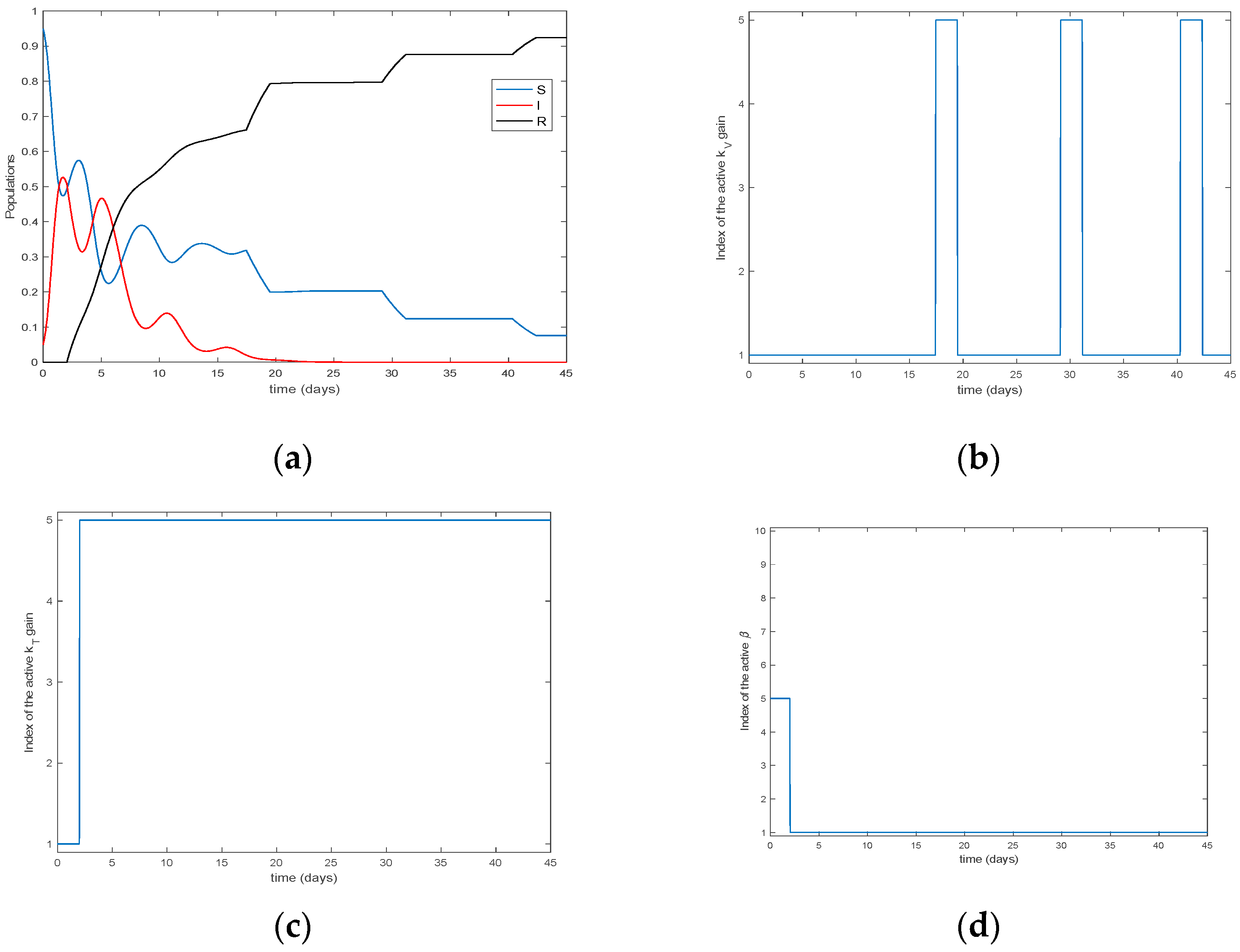
4. Simulation Results

This Section contains some simulation examples illustrating the switching algorithms introduced in Section 3. Thus, consider the model described by (1)–(3) with parameters given by $\beta =2.5$ and $\gamma =0.79$ in days ${}^{-1}$. These values have been inspired from [42] while the parameter $\beta$ has been increased in order to attain and endemic equilibrium point in the presented simulation examples. The model is normalized to unity and the initial conditions are $S(0)=0.95$ and $I(0)=0.05$, implying that the Susceptible are initially the 95% of the total population while the Infectious represent the 5%. In the absence of any external control action, the evolution of the system is displayed in Figure 1. As it can be observed in Figure 1, the compensatory immune subpopulation remains at zero at all time while the Susceptible and infectious converge to the endemic equilibrium point, characterized by an asymptotic nonzero infectious subpopulation. This situation corresponds to the case when the infection is persistent, since there exist a percentage of infectious individuals at the equilibrium, and external counteracting measurements have to be considered in order to eradicate the infection. It is observed in Figure 1 that the infection is persistent since there exists a percentage of infectious individuals at the equilibrium. To this end, vaccination and treatment are introduced in the model and orchestrated following the guidelines provided in Section 3.

In this way, consider the sets ${\mathit{S}}_{KV}={\mathit{S}}_{KT}=\left\{\begin{array}{ccccc}0& 0.001& 0.0035& 0.0075& 0.01\end{array}\right\}$ of potential feedback gains of vaccination and treatment, respectively. The initial value is zero, representing the case when no control action is taken, while the maximum value of these sets might be selected according to the maximum available resources (regarding the number of available vaccines or treatment doses) or by trial-error work. In this case, the sets are selected as example just to show the efficiency of the algorithms. With this choice there are 25 different elements in ${\mathit{S}}_{KV}\times {\mathit{S}}_{KT}$ leading to 25 different models, all of them parameterized by the same values for $\beta =2.5$ and $\gamma =0.79$. The initial conditions for all these models are $S_{ij}(0)=0.95$ and $I_{ij}(0)=0.05$ with $i,j=1,2,...,5$, where i is the index denoting the position of the gain from $S_{KV}$ while j is the index denoting the position of the gain from $S_{KT}$. If the Algorithm 1 of Section 3 with $T_{min}=2$ days and constant $\lambda =0.5$ is used, the evolution of the system is given in Figure 2a while the indexes that define the employed gains from the sets $S_{KV}$ and $S_{KT}$ are showed in Figure 2b,c, respectively. Figure 2d shows the evolution through time of the system under constant control gains of $k_V=k_T=0.001$.

It can be observed in Figure 2a that the control actions driven by Algorithm 1 are able to become the whole population immune asymptotically, removing the infection and making the Susceptible and the Infectious to vanish. Moreover, the evolution of the system under constant control gains of $k_V=k_T=0.001$ (the minimum non-zero values of the sets ${\mathit{S}}_{KV}$ and ${\mathit{S}}_{KT}$) is displayed in Figure 2d while the evolution of the system when $k_V=k_T=0.035$ is depicted in Figure 2e. It can be concluded that the selection of some constant values for the gains might lead to slower vanishing rates for the infectious, as it is observed from Figure 2a,d, while it might also lead to larger infective periods, as concluded from Figure 2a,e where it is seen that the infectious subpopulation vanishes at a later time when $k_V=k_T=0.035$ while the infection peak is smaller. Note also that larger constant control efforts can give fewer values of the infection peak but effectively damping the infection takes a longer time. See Figure 2a versus Figure 2e. Thus, the proposed algorithm allows designing epidemic counteracting actions without the necessity of performing extensive trial-error work in order to design appropriate gains to obtain a desired vanishing rate for the infectious, fulfilling hence the Objective 1 stated in Section 3 regarding the updated selection of appropriate control gains. Figure 3 displays the evolution of the system (the time evolution of Susceptible, Infectious and Immune) for different values of the weighting factor $\lambda =0,0.25,0.5,0.75,1$. It is observed that the evolution of the system is the same for $\lambda =0.5,0.75,1$ being all the plots superimposed for Susceptible, Infectious and Immune. Moreover, the higher vanishing rates for both the Susceptible and the Infectious are given for these latter values. Thus, a value of λ≥0.5 is recommended for the algorithm and $\lambda =0.5$ is used along this section.

Figure 4b,c show the indexes of the sets representing the gains at each time interval. It is observed in these figures that the convergence to the highest gain occurs at steps of size one. However, the transient behavior is worse for this case, as it can be deduced by comparing Figure 2a and Figure 4a. This happens because of the lower values for the control actions during the transient response in this last case in comparison with the standard Algorithm 1, as shown in Figure 5. The total vaccination and treatment efforts for Algorithm 1 are given by ${\displaystyle {\mathsf{\int }}_0^{40days}V(\tau )d\tau }=0.60$ and ${\displaystyle {\mathsf{\int }}_0^{40days}T(\tau )d\tau }=0.40$, respectively, while the efforts when the above variant is included are given by ${\displaystyle {\mathsf{\int }}_0^{40days}V(\tau )d\tau }=0.57$ and ${\displaystyle {\mathsf{\int }}_0^{40days}T(\tau )d\tau }=0.41$. From these values, calculated as the referred to time-integrals calculated over the control efforts which are obtained numerically from the simulation, it can be concluded that the total effort is not substantially improved when variations of one step are considered. Moreover, if vaccination and treatment resources are available it is recommendable to employ them as soon as possible since the maximum number of Infectious (peak of the infection) will be reduced and the duration of the infection will also be improved. Thus, the original description of Algorithm 1 outperforms the proposed variant.

Now, we consider the typical case when the transmission rate $\beta$ exhibits seasonal behavior. To this end, we consider the well-known Dietz’s model given by $\beta (t)={\beta }_0\left(1+Acos(2\pi ft)\right)$ in order to model the transmission rate with ${\beta }_0=2.5$, $A=0.6$ and $f=0.2$. The evolution of the system in the absence of external actions, when this incidence rate is used, is depicted in Figure 6, where the Immune are identically zero. As before, the infection is persistent since there always exist a positive number of infectious individuals and counteracting measurements are needed.

We consider now the set $S_{\beta }$ composed of 10 elements linearly spaced between ${\beta }_{min}={\beta }_0\left(1-A\right)$ and ${\beta }_{max}={\beta }_0\left(1+A\right)$. Under these circumstances, the Algorithm 2 may be used to select the most appropriate control gains. Thus, consider the 250 models contained in $S_{\beta }\times S_{KV}\times S_{KT}$ running in parallel. The same parameters as in the previous example are used and no variation is included in the algorithm. Figure 7a displays the evolution of the populations while the indexes corresponding to the active control gains and are given in Figure 7b–d. From Figure 7a it can be deduced that the switching rule is able to select the appropriate gains in order to eradicate the infection asymptotically.

A simulation example for Algorithm 3 is considered now. To this end, take $k_V^0=k_T^0=0$, $\mathrm{\Delta }{k}_V(0)=\mathrm{\Delta }{k}_T(0)=0.003$, the number of models is 6 for each gain set, ${\rho }_V^{}={\rho }_T^{}=0.001$ days ${}^{-1}$ and the same parameters as in the previous example. Therefore, the case of seasonal incidence rate is also considered here. The evolution of the system is depicted in Figure 8a. As before, the switching mechanism selects appropriate gains in order to remove the Infectious asymptotically. However, in this case the Susceptible do not converge to zero.

Figure 8 displays the control gains applied to the actual system. It can be seen that the vaccination remains zero at all time and the entropy-based approach selects only the application of treatment. This is the reason why the Susceptible do not converge to zero. Moreover, Figure 8c shows the time evolution of the treatment gain pointing out the fact that in this case the algorithm adapts the gains’ values through time.

Finally, an example of Algorithm 4 concludes this section. Thus, consider the same seasonal system as introduced in Algorithm 2. Now, according to Algorithm 4 there will be two models for each gain set initialized with $k_V(0)=k_T(0)=0$, $\mathsf{\Delta }{k}_V(0)=\mathsf{\Delta }{k}_T(0)=0.003$ and the same parameters as before. In this case the gains are updated through time by using a heuristic that takes into account the performance of the supervisory loss function in the previous switching times, as pointed out by equations in Algorithm 4, the evolution of the system is given in Figure 9a. Additionally, the values of the gains are depicted in Figure 9b,c. It can be deduced from these figures that the algorithm is able to eradicate the infection but the Susceptible do not converge to zero, neither. This happens because the algorithm selects to apply only the treatment action instead of both actions, vaccination and treatment, as Figure 9 shows. Moreover, the vanishing rate for the Infectious is smaller when using the Algorithm 4 in comparison to Algorithm 3. The main reason for this relies on the fact that the number of models is more reduced now since it goes from 36 of Algorithm 3 to just 4 of Algorithm 4. Hence, the computational burden is being reduced for Algorithm 4.

It can also be concluded from Figure 9c that the Algorithm is able to adapt the value of the gain to the appropriate one in order to eradicate the infection. In this Figure it can also be observed how the variation steps of the Algorithm decrease so that the change of the gain is smaller as time goes by. Figure 10a,b show the vaccination and treatment controls for Algorithms 2, 3 and 4. It can be noticed that Algorithms 3 and 4 only select the treatment action to deal with the persistency of the infections (i.e., the vaccination is identically zero) while Algorithm 2 selects both actions. As a consequence, the susceptible subpopulation does not converge to zero when using the last two algorithms.

On the other hand, the treatment action for Algorithms 2 and 3 is similar while Algorithm 4 applies a treatment action that is more extended in time resulting in larger infective periods. Thus, the peak of the action is smaller than in the previous approaches but it takes more time to eradicate the infection. In conclusion, the switching mechanisms presented in Section 3 based on the supervisory loss function frame are able to eradicate the infection by selecting the most appropriate gains at each time interval. Moreover, Figure 10 allows comparing the performance of Algorithms 2, 3 and 4 for the case of seasonality. It can be concluded that the smaller the control actions are, the larger the infectious subpopulation peak and the infective period are. Therefore, the selection of the algorithm can be conducted depending on the control objectives and the available resources.

This paper has been devoted to the investigation of supervisory techniques to update through time the feedback vaccination and control gains in a modified SI-epidemic model involving the susceptible and infectious subpopulations which is built from a basic uncontrolled SIS epidemic model. The presence of linear feedback controls motivates the incorporation of a new subpopulation to the basic model. Such an incorporated subpopulation is referred to as a compensatory recovered (or immune) one and it is subject to zero initial conditions. Therefore, the modified model is referred to as an SI (RC) epidemic model since it integrates susceptible, infectious and compensatory recovered subpopulations. The supervisory loss function can evaluate weighted losses involving the susceptible and the infectious subpopulations or, in particular, any of them only. The supervision problem is basically based on the implementation of a parallel control structure with different potential control gains to be judiciously selected and switched to be operated on the controlled model through time. A higher decision level structure selects the appropriate gains along a time interval and the time instants to switch between the successive active controllers in operation. Basically, switching to another controller on a time interval between two consecutive switching time instants is decided when a better supervisory loss value is detected associated with an alternative controller structure to that currently in operation within the parallel controllers’ disposal structure. Several algorithms for the design of the controller gains have been described and some numerical testing examples have also been given and discussed. The various proposed algorithms are able to: a) involve predefined set of gains; b) they can incorporate eventual variations of the transmission and recovery rates at the expense of a larger whole model complexity; c) they can update the control gains from a dynamic map of eventual candidates built from the current active ones; or d) the tests about switching the active parameterization decision might be performed at constant sampling periods.

A related future work is foreseen on the extension of the above method to other types of epidemic models which involve more subpopulations, e.g., several types of infected individuals, such as those exposed without symptoms which can later on have transitions to the infectious symptomatic and the infectious asymptomatic subpopulations. It is also intended to extend the above results to patchy environments where the disease is spreading in different regions, towns, etc., with mutual populations interchanges.

References

1. Khinchin, A.I. Mathematical Foundations of Information Theory; Dover Publications Inc.: New York, NY, USA, 1957. [Google Scholar]
2. Aczel, J.D.; Daroczy, Z. On Measures of Information and Their Generalizations; Academic Press: New York, NY, USA, 1975. [Google Scholar]
3. Ash, R.B. Information Theory; John Wiley and Sons: Hoboken, NJ, USA, 1965. [Google Scholar]
4. Feynman, R.P. Simulating Physics and Computers. Int. J. Theor. Phys. 1982, 21, 467–488. [Google Scholar] [CrossRef]
5. Burgin, M.; Meissner, G. Larger than one probabilities in mathematical and practical finance. Rev. Econ. Financ. 2012, 4, 1–13. [Google Scholar]
6. Tenreiro-Machado, J. Fractional derivatives and negative probabilities. Commun. Nonlinear Sci. Numer. Simul. 2019, 79, 104913. [Google Scholar] [CrossRef]
7. Baez, J.C.; Fritz, T.; Leinster, T. A characterization of entropy in terms of information loss. Entropy 2011, 13, 1945–1957. [Google Scholar] [CrossRef]
8. Delyon, F.; Foulon, P. Complex entropy for dynamic systems. Ann. Inst. Henry Poincarè Phys. Théorique 1991, 55, 891–902. [Google Scholar]
9. Nalewajski, R.F. Complex entropy and resultant information measures. J. Math. Chem. 2016, 54, 1777–2782. [Google Scholar] [CrossRef] [Green Version]
10. Goh, S.; Choi, J.; Choi, M.Y.; Yoon, B.G. Time evolution of entropy in a growth model: Dependence of the description. J. Korean Phys. Soc. 2017, 70, 12–21. [Google Scholar] [CrossRef] [Green Version]
11. Wang, W.B.; Wu, Z.N.; Wang, C.F.; Hu, R.F. Modelling the spreading rate of controlled communicable epidemics through and entropy-based thermodynamic model. Sci. China Phys. Mech. Astron. 2013, 56, 2143–2150. [Google Scholar] [CrossRef] [PubMed]
12. Tiwary, S. The evolution of entropy in various scenarios. Eur. J. Phys. 2020, 41, 025101. [Google Scholar] [CrossRef]
13. Koivu-Jolma, M.; Annila, A. Epidemic as a natural process. Math. Biosci. 2018, 299, 97–102. [Google Scholar] [CrossRef]
14. Artalejo, J.R.; Lopez-Herrero, M.J. The SIR and SIS epidemic models. A maximum entropy approach. Theor. Popul. Biol. 2011, 80, 256–264. [Google Scholar] [CrossRef]
15. Erten, E.Y.; Lizier, J.T.; Piraveenan, M.; Prokopenko, M. Criticality and information dynamics in epidemiological models. Entropy 2017, 19, 194. [Google Scholar] [CrossRef]
16. De la Sen, M. On the approximated reachability of a class of time-varying systems based on their linearized behaviour about the equilibria: Applications to epidemic models. Entropy 2019, 21, 1045. [Google Scholar] [CrossRef] [Green Version]
17. Li, K.; Small, M.; Zhang, H.; Fu, X. Epidemic outbreaks on networks with effective contacts. Nonlinear Anal. Real World Appl. 2010, 11, 1710–1725. [Google Scholar] [CrossRef]
18. Cui, Q.; Qiu, Z.; Liu, W.; Hu, H. Complex dynamics of an SIR epidemic model with nonlinear saturated incidence and recovery rate. Entropy 2017, 19, 305. [Google Scholar] [CrossRef]
19. Nistal, R.; De la Sen, M.; Alonso-Quesada, S.; Ibeas, A. Supervising the vaccinations and treatment control gains in a discrete SEIADR epidemic model. Int. J. Innov. Comput. Inf. Control 2019, 15, 2053–2067. [Google Scholar]
20. Verma, R.; Sehgal, V.K.; Nitin, V. Computational stochastic modelling to handle the crisis occurred during community epidemic. Ann. Data. Sci. 2016, 3, 119–133. [Google Scholar] [CrossRef]
21. Iggidr, A.; Souza, M.O. State estimators for some epidemiological systems. Math. Biol. 2019, 78, 225–256. [Google Scholar] [CrossRef] [Green Version]
22. Yang, H.M.; Ribas-Freitas, A.R. Biological view of vaccination described by mathematical modellings: From rubella to dengue vaccines. Math. Biosci. Eng. 2018, 16, 3185–3214. [Google Scholar]
23. De la Sen, M. On the design of hyperstable feedback controllers for a class of parameterized nonlinearities. Two application examples for controlling epidemic models. Int. J. Environ. Res. Public Health 2019, 16, 2689. [Google Scholar] [CrossRef] [Green Version]
24. De la Sen, M. Parametrical non-complex tests to evaluate partial decentralized linear-output feedback control stabilization conditions for their centralized stabilization counterparts. Appl. Sci. Basel 2019, 9, 1739. [Google Scholar] [CrossRef] [Green Version]
25. Meyers, L. Contact network epidemiology: Bond percolation applied to infectious disease prediction and control. Bull. Am. Math. Soc. 2007, 44, 63–86. [Google Scholar] [CrossRef] [Green Version]
26. De la Sen, M.; Alonso-Quesada, S.; Ibeas, A.; Nistal, R. On an SEIADR epidemic model with vaccination, treatment and dead-infectious corpses removal controls. Math. Comput. Simul. 2019, 163, 47–49. [Google Scholar] [CrossRef]
27. De la Sen, M.; Alonso-Quesada, S. Control issues for the Beverton-Holt equation in ecology by locally monitoring the environment carrying capacity: Non-adaptive and adaptive cases. Appl. Math. Comput. 2009, 215, 2616–2633. [Google Scholar] [CrossRef]
28. De la Sen, M.; Alonso-Quesada, S. Model-matching-based control of the Beverton-Holt equation in ecology. Discret. Dyn. Nat. Soc. 2008, 2008, 753912. [Google Scholar] [CrossRef]
29. De la Sen, M.; Ibeas, A.; Alonso-Quesada, S.; Nistal, R. On a SIR model in a patchy environment under constant and feedback decentralized controls with asymmetric parameterizations. Symmetry 2019, 11, 430. [Google Scholar] [CrossRef] [Green Version]
30. Herrmann-Pillath, C.; Salthe, S.N. Triadic conceptual structure of the maximum entropy approach to evolution. Biosystems 2011, 103, 315–330. [Google Scholar] [CrossRef] [Green Version]
31. Ulanowicz, R.E. The balance between adaptability and adaptation. Biosystems 2002, 103, 13–22. [Google Scholar] [CrossRef]
32. Toulias, T.L.; Kitsos, C.P. On the generalized lognormal distribution. J. Probab. Stat. 2013, 2013, 432642. [Google Scholar] [CrossRef] [Green Version]
33. Keeling, M.; Rohani, P. Modeling Infectious Diseases in Humans and Animals; Princeton University Press: Princeton, NJ, USA, 2008. [Google Scholar]
34. De la Sen, M.; Miñambres, J.J.; Garrido, A.J.; Almansa, A.; Soto, J.C. Basic theoretical results for expert systems. Applications to the supervision of adaptation transients in planar robots. Artif. Intell. 2004, 152, 173–211. [Google Scholar] [CrossRef] [Green Version]
35. De la Sen, M.; Agarwal, R.P.; Nistal, R.; Alonso-Quesada, S.; Ibeas, A. A switched multicontroller for an SEIADR epidemic model with monitored equilibrium points and supervised transients and vaccination costs. Adv. Differ. Equ. 2018, 2018, 390. [Google Scholar] [CrossRef]
36. De la Sen, M. Application of the non-periodic sampling to the identifiability and model-matching problems in dynamic systems. Int. J. Syst. Sci. 1983, 14, 367–383. [Google Scholar] [CrossRef]
37. De la Sen, M. Adaptive sampling for improving the adaptation transients in hybrid adaptive control. Int. J. Control 1985, 41, 1189–1205. [Google Scholar] [CrossRef]
38. Lee, T.H.; Xia, J.W.; Park, J.H. Networked control systems with asynchronous samplings and quantizations in both transmission and receiving channels. Neurocomputing 2017, 237, 25–38. [Google Scholar] [CrossRef]
39. Molla, M.K.I.; Ghosh, P.R.; Hirose, K. Bivariate MD- data adaptive approach to the analysis of climate variability. Discret. Dyn. Nat. Soc. 2011, 2011, 935034. [Google Scholar] [CrossRef]
40. Chen, J.; Meng, S.; Sun, J. Stability analysis of networked control systems with aperiodic sampling and time-varying delay. IEEE Trans. Cybern. 2017, 47, 2312–2320. [Google Scholar] [CrossRef]
41. Kim, J.; Park, J.; Shim, H.; Eun, Y. Zero-stealthy attack for sampled-data control systems: The case of faster actuation than sensing. In Proceedings of the 2016 IEEE 55th Conference on Decision and Control (CDC), Las Vegas, NV, USA, 12–14 December 2016; pp. 5956–5961. [Google Scholar]
42. Gao, N.; Song, Y.; Wang, X.; Liu, J. Dynamics of a stochastic SIS epidemic model with nonlinear incidence rates. Adv. Differ. Equ. 2019, 41, 19. [Google Scholar] [CrossRef] [Green Version]
Figure 1. Evolution of the populations for β = 2.5 and γ = 0.79 days 1 in the absence of external control actions, leading to a persistent infection.
Applsci 10 07183 g001
Figure 2. Performance of the system for β = 2.5 and γ = 0.79 days 1 when vaccination and treatment are included in the model. The control parameters are S K V = S K T = { 0 0.001 0.0035 0.0075 0.01 } , T m i n = 2 days and λ = 0.5 . The vaccination and treatment efforts are selected online via Algorithm 1. (a) Evolution of model’s populations. The infection is asymptotically removed while the whole population becomes immune asymptotically. (b) Index representing the active vaccination control gain versus time from S K V , parameterizing the vaccination effort. (c) Index representing the active treatment control gain versus time from S K T , parameterizing the treatment effort. (d) Evolution of model’s populations under constant control gains of k V = k T = 0.001 . (e) Evolution of model’s populations under constant gains of k V = k T = 0.035 .
Applsci 10 07183 g002
Figure 3. Evolution of the model’s populations for different values of λ and Algorithm 1. The model’s parameters are β = 2.5 and γ = 0.79 days 1 while T min = 2 days and S K V = S K T = { 0 0.001 0.0035 0.0075 0.01 } . (a) Susceptible. (b) Infectious. (c) Immune. It is interesting to notice that the switching mechanism based on the supervisory loss function selects the highest values for the feedback control gains (implying that Figure 2b,c are the same for both gains). This happens because a higher value for the control actions provokes a higher vanishing rate for Susceptible and Infectious, making the loss function to converge to zero as well (the minimum value of the loss function). Thus, the algorithm quickly selects the highest values. A variant of Algorithm 1 may be considered in order to avoid the fast convergence of the feedback gains to the maximum available value, implying the potential fast consumption of the available resources Thus, if the sets S K V and S K T are ordered we may only allow the switching in steps of one. This means that if the algorithm selects a gain that is more than one step ahead from the current active one, the algorithm is only allowed to move one position in the direction of the selected gain. If this variant is added in Algorithm 1 the closed-loop trajectories depicted in Figure 4a are obtained. It can be seen in Figure 4a that the Susceptible and the Infectious vanish while all the population becomes immune asymptotically.
Applsci 10 07183 g003
Figure 4. Performance of the system for β = 2.5 and γ = 0.79 days 1 when vaccination and treatment are included in the model. The control parameters are S K V = S K T = { 0 0.001 0.0035 0.0075 0.01 } , T min = 2 days and λ = 0.5 . The vaccination and treatment efforts are selected online via the variation of Algorithm 1 that only allows changes in steps of unity. (a) Evolution of model’s populations. (b) Index representing the active vaccination control gain versus time from S K V , parameterizing the vaccination effort. (c) Index representing the active treatment control gain versus time from S K T , parameterizing the vaccination effort.
Applsci 10 07183 g004
Figure 5. Comparison in the control efforts between Algorithm 1 and its proposed variation. (a) Vaccination. (b) Treatment.
Applsci 10 07183 g005
Figure 6. Evolution of the system when a seasonal incidence rate is employed.
Applsci 10 07183 g006
Figure 7. Performance of the system with seasonal incidence rate and vaccination and treatment actions tuned by Algorithm 2. (a) Evolution of model’s populations. (b) Index representing the active gain from S K V parameterizing the vaccination action. (c) Index representing the active gain from S K T parameterizing the treatment action. (d) Index representing the active model from S β parameterizing the transmission rate.
Applsci 10 07183 g007
Figure 8. Performance of the system with seasonal incidence rate and vaccination and treatment actions tuned by Algorithm 3. (a) Evolution of model’s populations. (b) Active gain from S K V parameterizing the vaccination action. (c) Active gain from S K T parameterizing the treatment action. (d) Index representing the active model from S β parameterizing the transmission rate.
Applsci 10 07183 g008
Figure 9. Performance of the system with seasonal incidence rate and vaccination and treatment actions tuned by Algorithm 4. (a) Evolution of model’s populations. (b) Active gain k V ( t ) . (c) Active gain k T ( t ) .
Applsci 10 07183 g009
Figure 10. Comparison of the performances obtained by Algorithms 2–4. (a) Vaccination functions. (b) Treatment functions. (c) Comparison of the evolution of Infectious.
Applsci 10 07183 g010
Publisher’s Note: MDPI stays neutral with regard to jurisdictional claims in published maps and institutional affiliations.