Abstract
This study analytically explored two coupled two-level atomic systems (TLAS) as two qubits interacting with two modes of an electromagnetic field (EMF) cavity via two-photon transitions in the presence of dipole–dipole interactions between the atoms and intrinsic damping. Using special unitary su Lie algebra, the general solution of an intrinsic noise model is obtained when an EMF is initially in a generalized coherent state. We investigated the population inversion of two TLAS and the generated quantum coherence of some partitions (including the EMF, two TLAS, and TLAS–EMF). It is possible to generate quantum coherence (mixedness and entanglement) from the initial pure state. The robustness of the quantum coherence produced and the sudden appearance and disappearance of coherence depended not only on dipole–dipole coupling but also on the intrinsic noise rate. The growth of mixedness and entanglement may be enhanced by increasing dipole–dipole coupling, leading to more robustness against intrinsic noise.
1. Introduction
Quantum entanglement (QE) is one of the main features of quantum information compared with classical information [1,2,3,4,5,6,7,8]. It describes nonlocal correlations [9] in quantum systems, which play major roles in quantum computation and quantum communication [10,11], teleportation [12,13,14,15], dense coding [16,17], and cryptography [18]. Thus, the purpose of this study was to explore methods of creating entangled states [19,20]. Von Neumann entropy, concurrence, and negativity are used to measure the properties of quantum coherence [21,22,23,24,25].
Matter-cavity interactions are used to produce entangled states [26,27,28] and are important examples of the physical realization of quantum information processing (QIP) [29]. The Jaynes–Cummings model (JCM) was introduced [30] to describe a two-level atomic system (TLAS) coupled to a single-mode radiation field. This model has attracted considerable attention for multi-photon transitions and interactions between TLAS and multi-mode EMFs [21]. Increasing the number of atoms interacting with an electromagnetic field (EMF) is another promising direction. Two TLAS with different extensions interacting with one-mode or two-mode fields have been investigated [22,31].
Many generalizations depending on the number of atomic levels, such as 2, 3, and 4-level atoms interacting with different types of cavity fields, have been investigated [22]. The quantum correlation dynamics between their subsystems (atom–atom, atom–field, and field–field) have also been studied [32]. The Kerr medium effects on the dynamics of nonlocal correlations between the two atoms that interact with a single mode field have also been studied [33]. Two TLAS interacting with a single mode vacuum field in the presence of atom–field and atom–atom entanglements were investigated using quantum relative entropy [22].
In real physical models, effective dissipation degrades the purity and entanglement [34,35,36,37,38,39,40]. One cause of dissipation is intrinsic decoherence in which the quantum effects deteriorate as the quantum system evolves. Intrinsic decoherence was studied in several previous articles [41,42,43,44,45,46,47]. Thus, this work introduces a physical model wherein the su-system is initially assumed to have a generalized coherent state, and an analytical description is used to investigate the entire system’s quantum coherence and its different partitions.
In this paper, the physical model is introduced in Section 2. The effects of the decay terms and dipole–dipole interactions on the atomic inversion of two atoms are studied in Section 3. The influences of the intrinsic dissipation and coupling rates between the two atoms on the purity are discussed in Section 4. In Section 5 and Section 6, QE in different partitions are investigated by using negativity measurements. Section 7 concludes this paper.
2. The Physical Model and Its Density Matrices
Much experimental work has been done on quantum entanglement using photons. It is worth noting that the individual polarization states of the photons can be easily controlled and their quantum coherence can be maintained over several kilometers in optical fibers [48]. Therefore, photons cannot be held for long time, and many difficulties arise in controlling collective entanglement states even if the photons are confined to the same cavity. It is interesting to note that the parametric amplifier type for an interaction between two fields can be realized in a three-wave mixing parametric amplifier device [49], and in quantum signals with Josephson circuits [50]. Therefore in this manuscript, the physical system of two two-level atomic systems, A and B, interacting with two nondegenerate modes of an EMF in an ideal cavity via four-photon transitions in the presence of dipole–dipole interactions is considered. The interaction that realizes nondegenerate parametric amplifier is an important nonlinear phenomenon [51,52]. The Hamiltonian that describes the parametric amplification interactions is expressed as
where and represent the field mode operators with frequencies of () and is the linear coupling parameter between the waveguide.
The model described by Equation (1) does not include any interactions with the two qubits. We posit that the two nondegenerate modes of the EMF in Equation (1) interact with the two coupled TLAS via dipole–dipole interactions. After applying rotating wave approximations, the model’s Hamiltonian becomes:
where represents the TLAS frequency and and are the Pauli matrices. is the coupling of the TLAS–EMF interactions and J is the coupling of the dipole–dipole interactions. If the two modes are identical, that is, , the degenerate two-photon transition of one field mode occurs in the Hamiltonian system in Equation () in the degenerate case.
We set and introduce the su generators and as follows:
which satisfies the relationship and . Therefore, is the Casimir operator and is the Bargmann number. The Hamiltonian of Equation () is governed by su and a su Lie algebra as:
Thus, the su operators in the number state representation induce the following operators:
Of note , the connection between the Bargmann number and the field modes’ photon number is .
In this study, we consider the intrinsic decoherence [41]. This decoherence is described by the Milburn equation, which is expressed as:
where is the intrinsic decoherence parameter. This equation is used to develop the density matrix approach to the dissipative systems. The solution of the previous differential Equation (6) through the Milburn equation can expressed as [41,53,54,55]:
where , and is the initial density system. Based on the completeness relation, , of the eigenvectors of the Hamiltonian system in Equation (4) into Equation (7); the density matrix is given by
where are the eigenvectors of the Hamiltonian (4) and are their corresponding eigenvalues. This density matrix is used to study the dynamical character of the quantum phenomena for different initial states where the coupling system is initially in the pure state . In the space states , the eigenstates are expressed as:
The coefficients satisfy , where is the eigenvalue of
It is worth mentioning that the eigenvectors of the Hamiltonian system in Equation (4) can be written by another symmetric combination of and [56] that will also be interesting for examining the behavior of the system when starting in an asymmetric correlated state.
We assume that the two su systems are initially in the upper state, , while the field system in the Barut–Girardello (BG) coherent states is [57],
with
where is the modified Bessel function
with
The su-system’s density matrix obtained by tracing over the TLAS A and B as:
where is the TLAS space states. The reduced density matrix of the TLAS is obtained by tracing the cavity field degrees that have space states as:
with
3. The Population Inversion of the Two TLAS
We now consider the atomic population inversion and discuss the behavior of the collapse and revival phenomena. The mathematical formula of atomic population inversion is the difference between the probabilities of finding the atom in excited and ground states. In this system, the two atoms are identical, so we can study the population of only one of the atoms in the su(2) subsystems—for example, A based on its reduced density matrix Tr. Therefore, the population inversion is expressed as:
As shown in Figure 1, the behavior of the function is illustrated with a fixed parameter , , and the other rates vary; specifically, and , which are related to the dissipation terms and dipole–dipole interactions, respectively. For example, for and , exhibits quasi-regular fluctuations between 1 and around the zero value. The population inversion demonstrates periods of revivals and collapses similar to the two-photon JCM [58]. When the dissipation term is taken into account, and , the amplitudes of the oscillations decrease as the scaled time increases; see Figure 1a
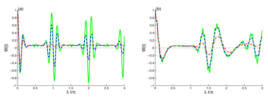
Figure 1.
The atomic inversion for and with different decoherence values of : (green solid curves), (blue dashed curves), and (red dashed dot curves) with in (a) and in (b).
Figure 1b shows the influence of the dipole–dipole rate in the absence of the dissipation terms. The function has irregular oscillations, and the amplitudes of the oscillations of decrease gradually as the time increases. When the influences of the rates of and are combined, the dipole–dipole interaction inhibits the fast deterioration of the damped oscillatory behavior of the atomic population inversion, which appears due to the dissipation term.
Figure 2a shows that the transfer of the energy between the upper atomic states and the lower states depends on the Bargmann number , where, with the increase of the Bargmann number k, the atomic population inversion is regular oscillatory behavior with a -period. The atomic system returns to its initial excited states periodically at the points . The influences of the initial coherent field intensity on the atomic population inversion dynamics are shown in Figure 2b for the case . We note that the increase of the initial coherent field intensity reduces the transfer process of the energy between the atomic states, and reduces the effect of the decoherence term. For the case , the dynamics of are more robust against intrinsic noise than those of the case of of Figure 1a.
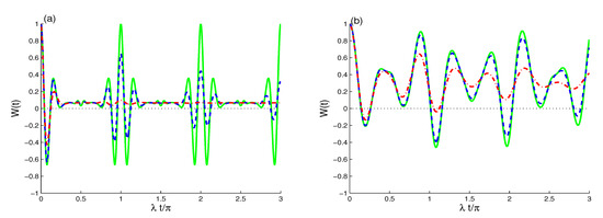
Figure 2.
As Figure 1a,b but for in (a) and in (b) with different decoherence values of : (green solid curves), (blue dashed curves), and (red dashed dot curves).
4. Coherence Loss Measures
The quantum coherence in the present system is due to: (1) The unitary TLAS–EMF interaction, in which the coherence is the QE between the atomic system and the cavity subsystems or is the coherence-loss for one of them. (2) The intrinsic decoherence leads to coherence-loss; in this case the coherence differs from the QE. Further, the effects of both the rates of dipole–dipole interactions and the decoherence on the quantum coherence were studied via the entire system’s von Neumann entropy, the EMF, and the TLAS.
- (1)
- The TLAS–EMF entropy is numerically calculated using the eigenvalues of the density matrix of the total system in Equation (13):
- (2)
The entropy functions , and satisfy the Araki-Lieb (A-LI) inequality as [60]:
If the dissipation term is neglected, Equation (11) is governed only by the unitary interactions of the TLAS–EMF system, so the TLAS–EMF system’s state is pure, . According to the A-LI inequality, Equation (22) becomes , and they are used to quantify the entanglement/mixedness. If the dissipation term is considered, then the TLAS–EMF state is a mixed; therefore, and , and the partial entropies are used to measure only the mixedness in the subsystems.
The numerical results of the entropy functions were obtained by numerically computing the eigenvalues of the density matrices of Equations (7), (10), and (11), and using the entropy Formulas (14) and (15). As shown in Figure 3, Figure 4 and Figure 5, the quantum coherence’s growth is analyzed by the functions , and using the same initial parameters as Figure 1. Since the atomic inversion’s revival periods decrease in the presence of the rates of the dipole–dipole interactions and the decoherence term, the TLAS–EMF system never reaches an initial pure state when the rates and are not equal to zero.
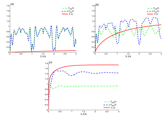
Figure 3.
The quantifiers (solid curves), (dash-dot curves), and (dash curves) for and . With different decoherence values: in (a), in (b), in (c).
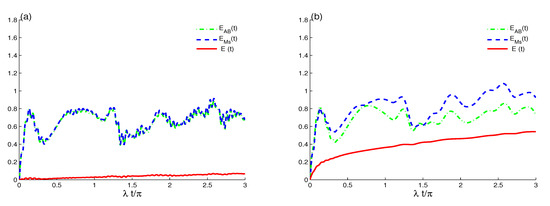
Figure 4.
As Figure 1 (a,b) but for .
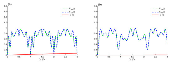
Figure 5.
As Figure 3 (a) but for different cases: in (a) and in (b).
Figure 3a shows the dynamics of the , , and in the absence of the dipole–dipole interactions and dissipation term. The TLAS, EMF, and TLAS–EMF systems’ states start from the initial pure states and evolve into mixed states. The entire entropy has small values compared with the values of and . The functions of and have approximately the same dynamic behavior and reach their minimal values at the middle point of the revival intervals, and the curves never reach their initial pure state, as shown in Figure 2a. Of note, the entropies gradually increase to their maximum values before and after the revival periods and then decrease to minimum values in the middle of the collapse periods.
Figure 3b,c shows that the dissipation term leads to a gradual increase in the , , and until they reach their time-independent stationary values, corresponding to the TLAS, EMF, and TLAS–EMF systems’ mixed states. The of the EMF system and its maximum values are greater than those of the TLAS. The amplitudes of the oscillations of and increase as the interaction time increases—that is, the system and its subsystems never come close to their initial pure states. The increase in the rate leads to growth of the entire entropy that is greater than growth for the partial entropies and . The entropy functions rapidly reach their stationary values.
As shown in Figure 4, the functions , , and are plotted at a dipole–dipole coupling and the other parameters are the same as in Figure 3a,b. The entropy functions and show rapid fluctuations with the interference between the patterns most of the time. For the small decay rate value , the growth of the entire entropy is less than that of the subentropies compared to in Figure 3b. We deduce that the dipole–dipole rate increases the chaotic oscillatory behavior of the entropy functions, and the generated mixedness of the TLAS and EMF states is more than that of the TLAS–EMF state.
Figure 5a shows the dynamics of the mixedness of the system and its subsystems for the case . By comparing this case with the case of Figure 3a, we find that the mixedness of the entropies is generated regular with -period, where the system and its subsystems are in initial pure states at the times . The effects of the initial coherent field intensity on the dynamics of the mixedness are shown in Figure 5a for the case . The small coherent field intensity leads to enhancing the generated mixedness and weakening the effect of the decoherence term.
5. The TLAS–EMF System’s Negativity Entanglement
Entanglement between the EMF and TLAS is quantified via the negativity of the total density matrix [61]. It is calculated using the matrix of the partial transposition of the density matrix in Equation (13) with respect to the TLAS states’ space . The matrix elements are expressed as:
The negativity’s close form is expressed as:
where represents the negative eigenvalues of the matrix . If , then the quantum state has maximal QE and it is zero for disentangled state; otherwise, the states have partial entanglement. The negativity will be calculated numerically by computing the negative eigenvalues of the matrix .
Figure 6, displays the effects of both the rates of intrinsic decoherence and the dipole–dipole interplay on the entanglement behavior between the EMF and TLAS with the same conditions using in the previous sections. In Figure 6a, is depicted when has different dissipation rate values . At , has regular oscillatory behavior with a -period. This behavior shows the ability of the unitary interactions between the EMF and TLAS to generate maximal and partial entanglement. The negativity gradually decreases to minimum values at the end of the period (where ) and reaches maximum values before and after the center of the revival periods, as shown in Figure 1a and Figure 6a. As the dissipation rate increases, the oscillations gradually decrease, and after a short time, the negativity damps the oscillatory behavior.
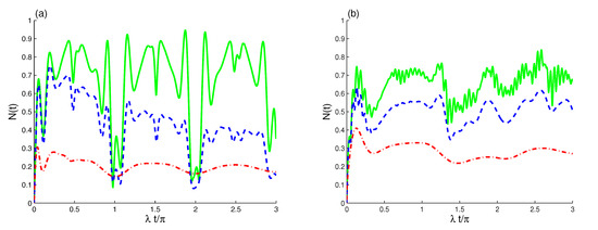
Figure 6.
The for and with different decoherence values of : (green solid curves), (blue dashed curves), and (red dashed dot curves). With in (a) and in (b).
The increase of leads to a decrease in the entanglement until it reaches its time-independent stationary non-zero value, which is called the stationary entangled state. The EMF and TLAS rapidly reach their stationary entangled states by increasing the decoherence rate.
Figure 6b displays the dynamic behavior of the TLAS–EMF entanglement with the rate of the dipole–dipole interactions . For small values of , exhibits more irregular oscillations. The maxima increased, whereas its minima shifted upward. This means that the dipole–dipole rate enhances the generated entanglement. We deduce that the effect of the rate is more pronounced due to the lesser development of the entanglement compared with the previous case . In general, the dipole–dipole rate increases entanglement, delaying the appearance of stationary entanglement.
Figure 7a illustrates that the regularity of the generated TLAS–EMF entanglement is enhanced under the effect of the Bargmann number for that case . The states of the atomic system and the two-mode coherent field cavity are disentangled periodically at the times . By comparing Figure 6a and Figure 7a, we find that the decoherence has the same effect on the dynamics of the generated TLAS–EMF entanglement. For the case where small initial coherent field intensity is considered, the generated TLAS–EMF entanglement can be enhanced compared to the case with large coherent field intensity.
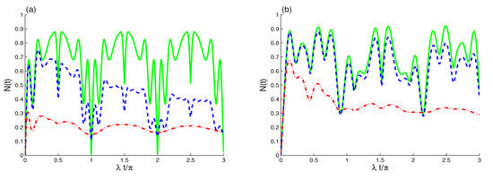
Figure 7.
As Figure 6 (a) but for different cases: in (a) and in (b) with different decoherence values of : (green solid curves), (blue dashed curves), and (red dashed dot curves).
6. Two-Atom System’s Entanglement
In the following section, the negativity function is used to study the QE of the two TLAS via the state in Equation (16). To calculate the negativity of the two TLAS, we find the partial transposition of the matrix with respect to the subsystem that is expressed by the following matrix:
where are the elements of in Equation (16). Then the TLAS negativity is computed numerically using , where is the negative eigenvalue of the matrix .
As shown in Figure 8, the effects of the rates of dipole–dipole interactions and dissipation term on the TLAS entanglement are displayed with the same conditions used in the previous section. As demonstrated in Figure 8a, in the absence of the dissipation rate, the negativity oscillates between its extreme values with regular oscillatory behavior, which shows the unitary interaction’s ability to generate TLAS entanglement. First, the negativity remains zero for a short period, until a particular time, when it suddenly increases from to its partial maximum value. After that, it decreases and suddenly disappears over a short period (the death period). The sudden appearance and disappearance of the entanglement [62,63,64] is repeated at further intervals of . The dissipative rate plays an important role in the negativity’s dynamic behavior. At low dissipation rates, fluctuates with no death periods over the course of the interactions. Larger values decrease the entanglement until it reaches its stationary state. Sudden appearance and disappearance does not occur.
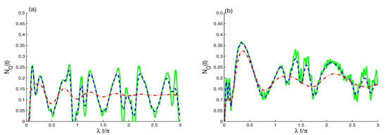
Figure 8.
The for and with different decoherence values of : (green solid curves), (blue dashed curves), and (red dashed dot curves). With in (a) and in (b).
Figure 8b, shows the behavior of the generated TLAS entanglement on the dipole–dipole rate when (). At low dissipation rates, the negativity demonstrates chaotic oscillatory behavior and never reaches zero (the disentangled state), as shown in Figure 8b. After the damping term is taken into account, the negativity increases and its minimum values are greater than those of in Figure 8a. The dipole–dipole rate increases the amplitudes and the negativity’s oscillations and also delays reaching stationary entanglement.
Figure 9a confirms that the Bargmann number has the same the effect on the previous quantum phenomena. For the case , the TLAS–EMF interactions lead to generate atomic entanglement periodically with -period. Compared to the case of Figure 8a, the time intervals of the sudden appearance and disappearance of the entanglement are increased clearly. Figure 9b shows that the ability of the TLAS–EMF interactions to generate the entanglement is weakened with the small initial coherent field intensity.
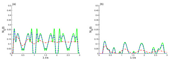
Figure 9.
As Figure 8 (a) but for different cases: in (a) and in (b) with different decoherence values of : (green solid curves), (blue dashed curves), and (red dashed dot curves).
Our results have potential applications in quantum information, such as: Generation of mixedness and entanglement under the decoherence [29]. The maximally entangled state of the two-qubit system can be used to employ quantum teleportation [65,66] or quantum dense coding [67]. The generated stable, maximally mixed state can be used to realize quantum computation [68,69] and qubit-channel metrology [70].
7. Conclusions
In the present context, the coupled TLAS interacting with two nondegenerate modes of an electromagnetic field represented by su(1,1) Lie algebra were investigated. The intrinsic damping effect of an effective dissipation term was studied by solving the Milburn equation. We investigated the effects of the dissipation and dipole–dipole rates on some quantum effects, namely, the atomic population inversion, quantum coherence, mixedness, and entanglement of the entire EMF and TLAS states. The atomic inversion’s revival and collapse periods depended on the dissipation and dipole–dipole rates. The dissipation and dipole–dipole rates may have controlled the behavior of some quantum effects that were measured using the negativity and von Neumann entropy. The oscillatory behavior of the different quantum effects and their stationary values were enhanced by the increase in the dipole–dipole rate. Through the results, we noticed clear effects of the dipole–dipole interaction and the decoherence on the phenomena of the collapses and revivals of the population inversion. Moreover, the oscillations decrease when increasing the dipole–dipole interaction and the function will fluctuate randomly. While increasing the decoherence, the amplitude of the oscillations decreases until it is erased after a short period of time. The entropies and negativity inspect the periodicity phenomenon and are generated mixedness and weaken the effect of the decoherence terms by adding the dipole–dipole interaction.
Author Contributions
The all authors contributed equally to the manuscript and typed, read, and approved the final manuscript. All authors have read and agreed to the published version of the manuscript.
Funding
Taif University Researchers Supporting Project number (TURSP-2020/17), Taif University, Taif, Saudi Arabia.
Acknowledgments
The authors are very grateful to the referees for their constructive remarks which have helped to improve the manuscript.
Conflicts of Interest
The authors declare no conflict of interest.
References
- Einstein, A.; Podolsky, B.; Rosen, N. Can Quantum-Mechanical Description of Physical Reality Be Considered Complete? Phys. Rev. 1935, 47, 777. [Google Scholar] [CrossRef]
- Brunn, N.; Cavalcanti, D.; Pironio, S.; Scarani, V.; Wehner, S. Bell nonlocality. Rev. Mod. Phys. 2014, 86, 419. [Google Scholar] [CrossRef]
- Streltsov, A.; Adesso, G.; Plenio, M.B. Colloquium: Quantum coherence as a resource. Rev. Mod. Phys. 2017, 89, 041003. [Google Scholar] [CrossRef]
- Vedra, V. Quantum entanglement. Nat. Phys. 2014, 10, 256. [Google Scholar] [CrossRef]
- Franco, R.L.; Compagno, G. Indistinguishability of Elementary Systems as a Resource for Quantum Information Processing. Phys. Rev. Lett. 2018, 120, 240403. [Google Scholar] [CrossRef] [PubMed]
- Sorelli, G.; Leonhard, N.; Shatokhin, V.; Reinlein, C.; Buchleitner, A. Entanglement protection of high-dimensional states by adaptive optics. New J. Phys. 2019, 21, 023003. [Google Scholar] [CrossRef]
- Rab, A.S.; Polino, E.; Man, Z.-X.; An, N.B.; Xia, Y.-J.; Spagnolo, N.; Franco, R.L.; Sciarrino, F. Entanglement of photons in their dual waveparticle nature. Nat. Commun. 2017, 8, 915. [Google Scholar] [CrossRef] [PubMed]
- Bellomo, B.; Franco, R.L.; Compagno, G. Nidentical particles and one particle to entangle them all. Phys. Rev. A 2017, 96, 022319. [Google Scholar] [CrossRef]
- Xu, J.-S.; Sun, K.; Li, C.-F.; Xu, X.-Y.; Guo, G.-C.; Andersson, E.; Franco, R.L.; Compagno, G. Experimental recovery of quantum correlations in absence of system-environment back-action. Nat. Commun. 2013, 4, 2851. [Google Scholar] [CrossRef]
- Barenco, A.; Deutsch, D.; Ekert, A.; Jozsa, R. Conditional Quantum Dynamics and Logic Gates. Phys. Rev. Lett. 1995, 74, 4083. [Google Scholar] [CrossRef]
- Bengtsson, I.; Zyczkowski, K. Geometry of quantum states: An Introduction to Quantum Entanglement; Cambridge University Press: Cambridge, UK, 2006. [Google Scholar] [CrossRef]
- Bennett, C.H.; Brassard, G.; Crepeau, C.; Jozsa, R.; Peres, A.; Wootters, W.K. Teleporting an unknown quantum state via dual classical and Einstein-Podolsky-Rosen channels. Phys. Rev. Lett. 1993, 70, 1895. [Google Scholar] [CrossRef] [PubMed]
- Ren, J.-G.; Xu, P.; Yong, H.-L.; Zhang, L.; Liao, S.-K.; Yin, J.; Liu, W.-Y.; Cai, W.-Q.; Yang, M.; Li, L. Ground-to-satellite quantum teleportation. Nature 2017, 549, 70. [Google Scholar] [CrossRef] [PubMed]
- Krauter, H.; Salart, D.; Muschik, C.A.; Petersen, J.M.; Shen, H.; Fernholz, T.; Polzik, E.S. Deterministic quantum teleportation between distant atomic objects. Nat. Phys. 2013, 9, 400. [Google Scholar] [CrossRef]
- Takeda, S.; Mizuta, T.; Fuwa, M.; van Loock, P.; Furusawa, A. Deterministic quantum teleportation of photonic quantum bits by a hybrid technique. Nature 2013, 500, 315. [Google Scholar] [CrossRef] [PubMed]
- Li, X.; Pan, Q.; Jing, J.; Zhang, J.; Xie, C.; Peng, K. Quantum Dense Coding Exploiting a Bright Einstein-Podolsky-Rosen Beam. Phys. Rev. Lett. 2002, 88, 047904. [Google Scholar] [CrossRef] [PubMed]
- Bennett, C.H.; Wiesner, S.J. Communication via one- and two-particle operators on Einstein-Podolsky-Rosen states. Phys. Rev. Lett. 1992, 69, 2881. [Google Scholar] [CrossRef] [PubMed]
- Ekert, A.K. Quantum cryptography based on Bell’s theorem. Phys. Rev. Lett. 1991, 67, 661. [Google Scholar] [CrossRef] [PubMed]
- Bose, S.; Knight, P.L.; Plenio, M.B.; Vedral, V. Proposal for Teleportation of an Atomic State via Cavity Decay. Phys. Rev. Lett. 1999, 83, 5158. [Google Scholar] [CrossRef]
- Mohamed, A.-B.A.; Eleuch, H. Generation and robustness of bipartite non-classical correlations in two nonlinear microcavities coupled by an optical fiber. J. Opt. Soc. Am. B 2018, 35, 47. [Google Scholar] [CrossRef]
- Khalil, E.M.; Abdalla, M.S.; Obada, A.-S.F. Pair entanglement of two-level atoms in the presence of a nondegenerate parametric amplifier. J. Phys. B At. Mol. Opt. Phys. 2010, 43, 095507. [Google Scholar] [CrossRef]
- Khalil, E.M.; Abdalla, M.S.; Obada, A.-S.F.; Perina, J. Entropic uncertainty in two two-level atoms interacting with a cavity field in presence of degenerate parametric amplifier. J. Opt. Soc. Am. B 2010, 27, 266. [Google Scholar] [CrossRef]
- Phoenix, S.J.D.; Knight, P.L. Establishment of an entangled atom-field state in the Jaynes-Cummings model. Phys. Rev. A 1991, 44, 6023. [Google Scholar] [CrossRef] [PubMed]
- Obada, A.-S.F.; Mohammed, F.A.; Hessian, H.A.; Mohamed, A.-B.A. Entropies and Entanglement for Initial Mixed State in the Multi-quanta JC Model with the Stark Shift and Kerr-like Medium. Int. J. Theor. Phys. 2007, 46, 1027. [Google Scholar] [CrossRef]
- Man, Z.-X.; Xia, Y.-J.; Franco, R.L. Cavity-based architecture to preserve quantum coherence and entanglement. Sci. Rep. 2015, 5, 13843. [Google Scholar] [CrossRef] [PubMed]
- Rogers, R.; Cummings, N.; Pedrotti, L.M.; Rice, P. Atom-field entanglement in cavity QED: Nonlinearity and saturation. Phys. Rev. A 2017, 96, 052311. [Google Scholar] [CrossRef]
- Mohamed, A.-B.A. Non-local correlations via Wigner Yanase skew information in two SC-qubit having mutual interaction under phase decoherence. Eur. Phys. J. D 2017, 71, 261. [Google Scholar] [CrossRef]
- Mohamed, A.-B.A.; Eleuch, H. Coherence and information dynamics of a Λ-type three-level atom interacting with a damped cavity field. Eur. Phys. J. Plus 2017, 132, 75. [Google Scholar] [CrossRef]
- Nielsen, M.A.; Chuang, I.L. Quantum Computation and Quantum Information; Cambridge University Press: Cambridge, UK, 2000. [Google Scholar]
- Jaynes, E.T.; Cummings, F.W. Comparison of quantum and semiclassical radiation theories with application to the beam maser. Proc. IEEE 1963, 51, 89. [Google Scholar] [CrossRef]
- Mohamed, A.-B.A. Bipartite non-classical correlations for a lossy two connected qubit–cavity systems: trace distance discord and Bell’s non-locality. Quantum Inf. Process. 2018, 17, 96. [Google Scholar] [CrossRef]
- Li, S.-B.; Xu, J.-B. Entanglement, Bell violation, and phase decoherence of two atoms inside an optical cavity. Phys. Rev. A 2005, 72, 022332. [Google Scholar] [CrossRef]
- Liu, T.K.; Wang, J.S.; Feng, J.; Zhan, M.S. Entropy evolution properties in a system of two entangled atoms interacting with light field. Chin. Phys. 2005, 14, 537. [Google Scholar]
- Obada, A.-S.F.; Hessian, H.A.; Mohamed, A.-B.A. Effect of phase-damped cavity on dynamics of tangles of a nondegenerate two-photon JC model. Opt. Commun. 2008, 281, 5189–5193. [Google Scholar] [CrossRef]
- Hessian, H.A.; Mohamed, A.-B.A. Quasi-probability distribution functions for a single trapped ion interacting with a mixed laser field. Laser Phys. 2008, 18, 1217–1223. [Google Scholar] [CrossRef]
- Shi, J.-D.; Xu, S.; Ma, W.-C.; Song, X.-K.; Ye, L. Purifying two-qubit entanglement in nonidentical decoherence by employing weak measurements. Quan. Inf. Procss. 2015, 14, 1387. [Google Scholar] [CrossRef]
- Obada, A.-S.F.; Hessian, H.A.; Mohamed, A.-B.A. The effects of thermal photons on entanglement dynamics for a dispersive Jaynes-Cummings model. Phys. Lett. A 2008, 372, 3699. [Google Scholar] [CrossRef]
- Aolita, L.; de Melo, F.; Davidovich, L. Open-system dynamics of entanglement: a key issues review. Rep. Prog. Phys. 2015, 78, 042001. [Google Scholar] [CrossRef]
- Dijkstra, A.G.; Tanimura, Y. Non-Markovian Entanglement Dynamics in the Presence of System-Bath Coherence. Phys. Rev. Lett. 2010, 104, 250401. [Google Scholar] [CrossRef]
- Franco, R.L.; Bellomo, B.; Maniscalco, S.; Compagno, G. Dynamics Of Quantum Correlations In Two-Qubit Systems Within Non-Markovian Environments. Int. J. Mod. Phys. B 2013, 27, 1345053. [Google Scholar] [CrossRef]
- Milburn, G.J. Intrinsic decoherence in quantum mechanics. Phys. Rev. A 1991, 44, 5401. [Google Scholar] [CrossRef]
- Mohamed, A.-B.A. Pairwise quantum correlations of a three-qubit XY chain with phase decoherence. Quantum Inf. Process. 2013, 12, 1141. [Google Scholar] [CrossRef]
- Obada, A.-S.F.; Abdel-Hafez, A.M.; Hessian, H.A. Influence of intrinsic decoherence on nonclassical effects in the nondegenerate bimodal multiquanta Jaynes-Cummings model. J. Phys. B 1998, 31, 5085. [Google Scholar] [CrossRef]
- Raja, S.H.; Mohammadi, H.; Akhtarshenas, S.J. Geometric discord of the Jaynes-Cummings model: Pure dephasing regime. Eur. Phys. J. D 2015, 69, 14. [Google Scholar] [CrossRef]
- Mohamed, A.-B.; Farouk, A.A.; Yassen, M.F.; Eleuch, H. Quantum Correlation via Skew Information and Bell Function Beyond Entanglement in a Two-Qubit Heisenberg XYZ Model: Effect of the Phase Damping. Appl. Sci. 2020, 10, 3782. [Google Scholar] [CrossRef]
- Mohamed, A.-B.; Eleuch, A.H.; Raymond Ooi, C.H. Non-locality Correlation in Two Driven Qubits Inside an Open Coherent Cavity: Trace Norm Distance and Maximum Bell Function. Sci. Rep. 2019, 9, 19632. [Google Scholar] [CrossRef] [PubMed]
- Mohamed, A.-B.; Eleuch, A.H.; Raymond Ooi, C.H. Quantum coherence and entanglement partitions for two driven quantum dots inside a coherent micro cavity. Phys. Lett. A 2019, 383, 125905. [Google Scholar] [CrossRef]
- Giovannetti, V.; Lloyd, S.; Maccone, L. Quantum-enhanced positioning and clock synchronization. Nature 2001, 412, 417. [Google Scholar] [CrossRef] [PubMed]
- Franken, P.A.; Hill, A.E.; Peters, C.W.; Weinreich, G. Generation of Optical Harmonics. Phys. Rev. Lett. 1961, 7, 118. [Google Scholar] [CrossRef]
- Roy, A.; Devoret, M. Introduction to parametric amplification of quantum signals with Josephson circuitsIntroduction a lamplification parametrique de signaux quantiques par les circuits Josephson. Comptes Rendus Phys. 2016, 17, 740. [Google Scholar] [CrossRef]
- Rekdal, P.K.; Skagerstam, B.-S.K. Quantum Dynamics of Non-Degenerate Parametric Amplification. Phys. Scr. 2000, 61, 296. [Google Scholar] [CrossRef]
- Dehghani, A.; Braz, B.M. Minimum Uncertainty Coherent States Attached to Nondegenerate Parametric Amplifiers. Braz. J. Phys. 2015, 45, 265. [Google Scholar] [CrossRef]
- Gardiner, C.W. Quantum Noise; Springer: Berlin, Germany, 1991. [Google Scholar]
- Moya-Cessa, H.; Buzek, V.; Kim, M.S.; Knight, P.L. Intrinsic decoherence in the atom-field interaction. Phys. Rev. A 1993, 48, 3900. [Google Scholar] [CrossRef] [PubMed]
- Xu, J.-B.; Zou, X.-B. Dynamic algebraic approach to the system of a three-level atom in the Λ configuration. Phys. Rev. A 1999, 60, 4743. [Google Scholar] [CrossRef]
- de los Santos-Sánchez, O.; Gonzxaxlez-Gutiérrez, C.; Rxexcamier, J. Nonlinear Jaynes—Cummings model for two interacting two-level atoms. J. Phys. B At. Mol. Opt. Phys. 2016, 49, 165503. [Google Scholar]
- Barut, A.O.; Girardello, L. New “coherent” states associated with non-compact groups. Commun. Math. Phys. 1971, 21, 41. [Google Scholar] [CrossRef]
- Gerry, C.C.; Moyer, P.J. Squeezing and higher-order squeezing in one- and two-photon Jaynes-Cummings models. Phys. Rev. A 1988, 38, 5665. [Google Scholar] [CrossRef]
- Bennett, C.H.; Bernstein, H.J.; Popescu, S.; Schumacher, B. Concentrating partial entanglement by local operations. Phys. Rev. A 1996, 53, 2046. [Google Scholar] [CrossRef]
- Araki, H.; Lieb, E. Entropy inequalities. Commun. Math. Phys. 1970, 18, 160. [Google Scholar] [CrossRef]
- Vidal, G.; Werner, R.F. Computable measure of entanglement. Phys. Rev. A 2002, 65, 032314. [Google Scholar] [CrossRef]
- Eberly, J.H.; Yu, T. The End of an Entanglement. Science 2007, 316, 555. [Google Scholar] [CrossRef]
- Yu, T.; Eberly, J.H. Sudden Death of Entanglement. Science 2009, 323, 598. [Google Scholar] [CrossRef]
- Mohamed, A.-B.A.; Hessian, H.A.; Obada, A.-S.F. Entanglement sudden death of a SC-qubit strongly coupled with a quantized mode of a lossy cavity. Physica A 2011, 390, 519. [Google Scholar] [CrossRef]
- Xu, H.; Yong, L.; Liao, S.; Yin, J.; Cai, W.; Yang, M.; Li, L.; Yang, K.; Han, X.; Yao, Y.; et al. Ground-to-satellite quantum teleportation. Nature 2017, 549, 70. [Google Scholar]
- Chou, K.S.; Blumoff Jacob, Z.; Wang, C.S.; Reinhold, P.C.; Axline, C.J.; Gao, Y.Y.; Frunzio, L.; Devoret, M.H.; Jiang, L.; Schoelkopf, R.J. Deterministic teleportation of a quantum gate between two logical qubits. Nature 2018, 561, 368. [Google Scholar] [CrossRef] [PubMed]
- Nielsen, M.A.; Chuang, I.L. Application: Superdense Coding. Quantum Computation and Quantum Information, 10th ed.; Cambridge University Press: Cambridge, UK, 2010. [Google Scholar]
- Siomau, M.; Fritzsche, S. Quantum computing with mixed states. Eur. Phys. J. D 2011, 62, 449. [Google Scholar] [CrossRef]
- Hou, S.-Y.; Sheng, Y.-B.; Feng, G.-R.; Long, G.-L. Experimental Optimal Single Qubit Purification in an NMR Quantum Information Processor. Sci. Rep. 2015, 4, 6857. [Google Scholar] [CrossRef] [PubMed]
- Collins, D. Qubit-channel metrology with very noisy initial states. Phys. Rev. A 2019, 99, 012123. [Google Scholar] [CrossRef]
Publisher’s Note: MDPI stays neutral with regard to jurisdictional claims in published maps and institutional affiliations. |
© 2020 by the authors. Licensee MDPI, Basel, Switzerland. This article is an open access article distributed under the terms and conditions of the Creative Commons Attribution (CC BY) license (http://creativecommons.org/licenses/by/4.0/).